
43
PROCESS MODELING APPLICATIONS TOWARD ENABLING DEVELOPMENT AND SCALE‐UP: CHEMICAL REACTIONS
Anuj A. Verma, Steven Richter, Brian Kotecki, and Moiz Diwan
Process Research and Development, AbbVie Inc., North Chicago, IL, USA
43.1 INTRODUCTION
With an increase in the number of pipeline compounds in CMC development among pharmaceutical companies that need to be delivered using limited pool of resources, efficient tools for process understanding need to be established to enable predictive scale‐up of chemical reactions in the pilot plant and in manufacturing. Process modeling is an example of such efficient tools available among the chemical engineering community. Through an appropriate application of this tool, a process engineer can obtain multivariate understanding of the various factors affecting the scale‐up of a chemical reaction with limited data. Process models can further assist in simulating the impact of various process parameters on quality target product profile. As a result, an appreciable number of pharmaceutical companies have dedicated resources to modeling chemical reaction processes toward enabling development and scale‐up.
Process modeling of chemical reactions uses mathematical principles of chemical reaction engineering to prepare mechanistic multivariate models that agree with experiment. A typical roadmap of such an analysis is shown in Figure 43.1.
FIGURE 43.1 Typical roadmap for process modeling in chemical reaction engineering.
An aim for a process modeler is to assess the suitability or robustness of a contacting device that conducts the chemistry of interest with regard to three major areas of investigation: kinetics and thermodynamics, heat and mass transfer, and flow patterns. Having a multivariate understanding of these factors enables understanding of the fate of chemical reaction as the reactant is converted to product, by‐products, and impurities. A brief description of these areas of investigation is provided below:
- Kinetics and thermodynamics. The analysis of intrinsic reaction kinetics and chemical reaction equilibria enables a process modeler to assess the forward and net rate of conversion of a starting material to product/impurity in the absence of mass transfer limitations. For example, in a simplistic example of bimolecular second‐order reactions, kinetics provide a measure of the probability of a successful collision that forms the product/impurity out of all the collisions between the two sets of molecules. These probabilities change with concentration and reaction temperature and are generally described adequately by the Arrhenius equation coupled with chemical reaction equilibria.
- Transport phenomena. Analysis of transport phenomena enables a process modeler to assess the total number of molecular collisions (irrespective of number of successful collisions leading to a chemical reaction). This is typically calculated as the rate at which the contacting device can bring the reacting molecules to collide and is a function of mixing intensity in a single phase and interphase transport rate in a multiphase reaction. This rate is always greater than or equal to the rate of chemical reaction involving bimolecular collisions. Mixing also affects the heat distribution locally in an exothermic or endothermic chemical reaction. This is shown mathematically by similar dimensionless equations of heat and mass transport locally in a differential fluid volume [1]. Moreover, this analysis has a direct impact on the kinetics of reaction due to its ability to map out the variation of concentration of chemical entities and temperature in the contacting device. Under a large number of practical scenarios, computational fluid dynamics (CFD) becomes an important tool for understanding transport phenomena.
- Flow patterns. Most analysis of kinetics and transport phenomena locally depends on the reaction fluid following a variation of an ideal flow pattern, i.e. plug flow (in a plug flow reactor [PFR]) or perfectly back‐mixed flow (in a CSTR). In real contacting devices, however, the analysis of flow patterns is paramount to the performance of the same because these flow patterns and other system nonidealities (like dead volumes and recirculation zones) affect the generation of impurities and by‐products. Often, based on the kinetics of impurity generation, or from an operational viewpoint (slurry processing, for example), a particular flow pattern can be desired. As a result, a systematic analysis of global flow patterns in the contacting device helps to ensure robustness of the reaction process with respect to impurity/by‐product generation. In flow reactors, a combination of kinetics and transport phenomena can help in guiding the desirable flow patterns in a continuous reactor that maximize yield and minimize impurities.
This chapter provides three detailed examples where the chemical reaction process modeling roadmap has been utilized to design and understand the robustness of respective contacting devices in order to enable predictive scale‐up of business‐relevant chemical transformations.
43.2 PREDICTIVE SCALE‐UP OF A HIGHLY EXOTHERMIC REACTION
43.2.1 Introduction
In the pharmaceutical industry, the focus of process development shifts from obtaining an adequate yield and quality in a chemical reaction in early stage (before phase I clinical readout) to a robust process with a proper understanding of critical quality attributes (CQAs) on reaction performance and product quality in later stages (phase II clinical readout and beyond). For late‐stage development, chemical reactions can be challenging to scale‐up due to a lack of fundamental understanding of the impact of transport phenomena in impurity generation and overall robustness of the reaction process. Herein, we apply the reaction process modeling roadmap to an example of a mixing sensitive mesylation reaction in a late‐stage drug substance process. The reaction pathway is shown in Scheme 43.1.

SCHEME 43.1 Reaction of an alcohol with methanesulfonyl chloride (MsCl). The solvent has an alternate reaction with MsCl.
43.2.2 Problems Faced in Reaction Scale‐up
Methanesulfonyl chloride (MsCl) undergoes a fast reaction with starting material alcohol in the presence of triethylamine to form the desired product and triethylammonium hydrochloride salt. This reaction is very exothermic with a 250 kJ/mol heat of reaction and an adiabatic temperature rise (ATR) of 120 °C in that solvent. On the other hand, methanesulfonyl chloride also reacts with the solvent to form an impurity (Scheme 43.1). A fed‐batch process was developed with slow dosing of MsCl to keep the overall reaction temperature at less than 10 °C (Figure 43.2). Due to the side reaction with the solvent, early process development work recommended the use of 1.3 equiv of MsCl. Further lowering the MsCl equivalents led to incomplete conversion, while higher equivalents led to additional impurity generation. It was desired that the reaction endpoint would have no more than 2% starting material alcohol remaining in the reaction mixture (>98% conversion). A higher level of remaining starting material alcohol and an increased impurity burden were separately shown to have an inadequate purge in downstream processing.
FIGURE 43.2 Process diagram for the mesylation reaction in a fed‐batch reactor.
Preliminary reaction scale‐up in fed‐batch reactors of increasing sizes (1–1000 L) revealed undesirable scale‐up effects. There were instances of reaction stalling at suboptimal conversion of the alcohol. These batches would be subjected to additional charges of MsCl, leading to increased impurity levels. Due to these variabilities, there was risk of failing reaction endpoint specification. This was concerning as the reaction was a part of a late‐stage compound and this observation would hamper efficient technology transfer to the manufacturing site. As a result, the reaction process modeling roadmap was applied to provide reaction robustness and enable efficient technology transfer to manufacturing site.
43.2.3 Analysis of Transport Phenomena
Early process development work pointed toward the reaction being mixing limited. In phenomenological terms, the observed rate of reaction was equal to the rate of mixing locally in the contacting device. This can be characterized mathematically by using the reaction Damköhler number defined by Eq. (43.1). In other words, the reaction Damköhler number was greater than one:
If proper mixing protocols are not followed at different scales of operation, there could be concentration and temperature gradients (due to high exothermicity of the reaction). The presence of local hotspots was more concerning due to possibility of preferential impurity generation and loss of MsCl toward the main reaction. This problem was expected to become worse with increasing reaction scale. In order for the reaction to be robust upon scale‐up, a quantitative fit‐for‐purpose analysis of the mixing in the contacting device (stirred reactor) was needed. This exercise would provide for a reasonable scale‐independent measure of mixing time to ensure a passing reaction endpoint.
The quantification of mixing was assessed by mixing time scales during chemical reaction (Figure 43.2). In general, three mixing time scales can be quantified in a stirred vessel. Its quantification is provided by the Baldyga and Bourne mixing model, and the full details of this model are provided in Ref. [2]. A short description of the different mixing time scales is provided below:
- Micromixing engulfment time. The micromixing engulfment time scale is the inverse of the rate of mixing in fluid packets that have a length scale smaller than the Kolmogorov length [1]. Below this length scale, the main mode of mixing is laminar. Large‐scale eddies break down to below the Kolmogorov scale where mixing continues and is governed by laws of laminar mixing. The micromixing time scale defined by Bourne and Baldyga is shown below:(43.2)
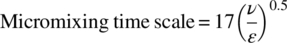
The rate of mixing, which is the inverse of this micromixing time scale, depends on the kinematic viscosity (ν) and the dissipation rate of turbulent kinetic energy (per unit mass, ε) in those fluid packets. This rate of mixing affects both the mass and heat transfer.
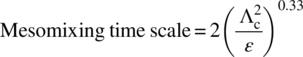
- Mesomixing time. The mesomixing time scale is the inverse of rate of mixing in fluid packets having a length scale larger than the Kolmogorov scale but smaller than the contacting device length scale (typically the diameter of the stirred tank). The main mechanism of mixing occurs through convective transport phenomena and is turbulent in nature. The typical length scales of mesomixing (Λc) depend on the relative measure of the reagent dose rate (QB) compared to the main reactor surrounding fluid velocity (u). For relatively small dose rates, Λc is provided by Eq. (43.4), while for dose velocity (u = QB/Apipe) comparable with the velocity of surrounding fluid, Λc is close to the feed pipe diameter:
Hence these time scales depend mainly on the dissipation rate of turbulent kinetic energy and an intermediate measure of length. There is a possibility that upon scale‐up, a mixing‐limited reaction can change their mechanism from being micromixing limited in the laboratory to being mesomixing limited in the plant. Hence, one must always analyze micromixing and mesomixing time scales together and be observant on possible changes in rate‐limiting steps.
- Blend time. It is the time taken by the fluid to be homogeneous in the length scale of the entire vessel. This time scale is usually higher than either the micromixing or the mesomixing time scales.

For mixing‐limited reactions with Da > 1, the time scale of the reaction is usually compared and ranked with either micromixing time, mesomixing time, or blend time. A controlling mechanism is inferred, and appropriate scale‐up guidance is provided. For our reaction of interest, the relative measures of these time scales are provided in Table 43.1.
TABLE 43.1 Tabulation of Reaction Conversion with Micromixing and Mesomixing Time Scales in Different‐Sized Reactors
| Impeller RPM | Reactor Volume (L) | Mesomixing Time (s) | Micromixing Time (s) | Conversion (Peak Area %) |
| 103 | 0.1 | 0.17 | 2.51 | 99.05 |
| 401 | 0.1 | 0.03 | 0.33 | 99.86 |
| 100 | 0.1 | 0.17 | 2.51 | 99.49 |
| 50 | 0.1 | 0.44 | 7.42 | 98.4 |
| 210 | 0.1 | 0.07 | 0.86 | 99.73 |
| 82 | 0.1 | 0.25 | 3.53 | 98.47 |
| 77 | 0.1 | 0.28 | 3.88 | 99.22 |
| 50 | 0.5 | 0.71 | 8.01 | 97.47 |
| 90 | 1050 | 0.18 | 0.24 | 99 |
| 94 | 1050 | 0.17 | 0.22 | 99.8 |
| 90 | 1050 | 0.18 | 0.24 | 99.3 |
The analysis of fluid mixing rates also provides for a direct correlation with the temperature inhomogeneity at appropriate reaction scales as shown in Figure 43.3. This is due to the similarity of the dimensionless equations of local heat and mass transfer with respect to fluid mixing [1]. Suppose a fluid packet is at temperature T with the surrounding fluid at temperature <T> (≠T). A lower rate of mixing leads to a suboptimal rate of swirling of the surrounding fluid into the test fluid packet to equalize the temperature. This leads to lower heat transfer rates and temperature inhomogeneity. For our example, temperature “hotspots,” in addition to mass transfer inhomogeneity, could potentially lead to MsCl being consumed in unproductive pathways.
![Schematic depicting a square labeled T [Ai] and pointed by arrows labeled <T>, <[u]>, and <[Ai}>. On top are C-shapes indicating Ac.](http://images-20200215.ebookreading.net/2/1/1/9781119285861/9781119285861__chemical-engineering-in__9781119285861__images__c43f003.gif)
FIGURE 43.3 Use of mixing time scale to correlate with the local temperature excursion in the exothermic reaction.
Returning to Figure 43.3, an analysis of mixing time scales was to be done in the zone of chemical reaction within the stirred reactor. A best‐case scenario for fluid mixing is to dose the MsCl subsurface very close to the impeller. This configuration effectively utilizes the highest rate of mixing due to very high levels of turbulence generated close to the impeller. Manufacturing limitations, however, prevented this configuration and restricted the MsCl dosage to be above surface. One main reason for this restriction was that substantial efforts would be required to retrofit the subsurface dip tube with a nozzle of appropriate diameter to effectively prevent the reactive mixture to diffuse into the tube. Applying the Baldyga and Bourne mixing model [2], three key requirements for mixing analysis are the kinematic viscosity, mesomixing length scale (Λc), and turbulent dissipation rate at the location on the liquid surface where the drop impinges. The kinematic viscosity of the endpoint reaction mixture was experimentally obtained from a rheometer in the laboratory at process‐relevant temperatures. The dissipation rate of turbulent kinetic energy (ε) was calculated by the following relation:
where
- εimpeller was the turbulence generated by the action of the impeller at the feed location on the liquid surface and was calculated by CFD applied to reactors of various sizes of interest.
- εfeed jetting was the turbulence generated by the accelerating above‐surface drop in a gravitational field, whose value is provided by Newton’s laws.
- εbuoyancy was the turbulence generated by the difference in buoyancy between the droplet and the reaction liquid. This was once again provided by Newton’s laws.
It should be emphasized that εfeed jetting + εbuoyancy was less than 3% contribution to the total turbulence intensity and was negligible in comparison with the turbulence provided by the impeller.
The mesomixing length scale was calculated by estimating the surrounding fluid velocity in the reaction zone via CFD and using Eq. (43.4) for a known dose volumetric flow rate of MsCl.
These values were subsequently input in a DynoChem mixing utility to calculate the micro‐ and mesomixing time scales for various reactor configurations and various intensities of agitation during the experiment. The three volume scales that were experimentally evaluated were 0.1, 0.5, and 1000 L.
43.2.4 Results
Table 43.1 and Figure 43.4 display the results from various experiments conducted in the laboratory with different impeller speeds (to simulate different mixing time scales) and pilot‐scale campaigns.

FIGURE 43.4 Variation of the conversion of alcohol with mesomixing time for different reactor scales.
From Figure 43.4, an increase in mesomixing time caused a linear decrease in reaction conversion. This was consistent with the expectation that longer mixing times lead to more inhomogeneity in temperature and concentration across the reactor, leading to progressively more suboptimal usage of MsCl. To demonstrate that this measure of reaction mixing time scale was an appropriate scale‐independent parameter, a representative experiment was performed at a higher scale in the laboratory (0.5 versus 0.1 L), and the reaction performance scaled appropriately (as shown in Figure 43.4). Based on these recommendations, three clinical trial supply batches executed in the pilot plant at 1050 L scale also provided passing results consistently.
Separately, an analysis of micromixing time scales in the same experiments revealed that the reaction is not limited by micromixing. Figure 43.5 shows the variation of the reaction conversion with the change in micromixing time scale.
FIGURE 43.5 Variation of conversion of alcohol versus the micromixing time scale. These experiments were performed at the same mesomixing time scale (0.17 s).
A 10‐fold change in micromixing rate led to almost no change in reaction conversion. This was consistent with the reaction Da ≫ 1 as a result of which the reaction volume was differentially small and localized even at 1000 L scale. Due to this localization, bulk of the heat and mass transfer was to be accomplished when the MsCl droplet enters the mesoscale and completes the reaction in those scales. Otherwise, MsCl droplet would have continued to react below the Kolmogorov scale (microscale), and a deleterious effect on reaction conversion would have been seen by increasing the micromixing time scale.
Thus, the reaction process was judged to be limited by the rate of mesomixing. From Figure 43.5, a scale‐independent mesomixing time can be specified with limits, thereby forming a mixing‐based design space. For the chemistry of interest, a maximum mesomixing time scale corresponding to 0.4 second at the feed location (or a minimum mesomixing rate = 2.5 s−1) was identified, which provided a passing conversion of greater than 98% of the alcohol. Efficient technology transfer to different reactors of interest was accomplished by dictating a scale‐independent mesomixing time requirement of 0.2 second (or less). With this number, a process engineer can perform predictive technology transfer in the following way:
- Obtain complete reactor geometry and perform CFD simulations to map out the dissipation rate of turbulent kinetic energy and fluid velocities, and obtain those values near the feed location.
- Dictate that near the feed location, we want a mesomixing time scale of 0.2 second.
- Using Eq. (43.4) and CFD simulations, obtain a desired mesomixing length and turbulent dissipation energy.
- Refine the CFD simulations till optimal values of mesomixing length and turbulent dissipation energy are obtained.
- Finalize the impeller RPM and MsCl dose rate.
43.2.5 Conclusions
Rational analysis of transport phenomena revealed that the variability in reaction conversion was due to the reaction being mesomixing limited. As the scale of operation increased, there is increased variability in temperature and mass inhomogeneity, leading to suboptimal usage of MsCl, which decreased conversion and increased impurity generation. Using the approach highlighted in this example, proper scale‐up guidance was provided to enable successful technology transfer to the manufacturing site with consistent reaction performance.
43.3 EFFICIENT SCALE‐UP OF A MULTIPHASE EXOTHERMIC NITRATION REACTION
43.3.1 Introduction
The nitro derivatives of aromatic compounds are frequently used as intermediates to form amines in the pharmaceutical industry. These reactions, however, are very energetic, producing a powerful exotherm that can be hard to control upon reaction scale‐up. Moreover, there is potential for over‐nitration. This leads to a safety concern because dinitro and trinitro compounds are often labeled as explosives by the safety laboratory. As a result, the level of over‐nitrated compounds has to be controlled via a strict control of nitration stoichiometry along with a preference of performing flow chemistry for such reactions [3–5]. The advantages of flow chemistry for nitration include high rates of heat and mass transfer caused by higher rates and more homogeneous mixing compared with batch reactors. Among flow chemistry contacting devices, many academic groups preferred the use of microreactors [4, 6, 7]; however, more industrial nitration reactors are composed of coiled metallic pipes and CSTRs [3, 8].
Although there have been various successful demonstrations of continuous flow nitration [3–8], a rational mathematical framework to evaluate the scale‐up of such reactions in the pharmaceutical setting has been missing. In this example, nitration of 4‐trifluoromethyl toluene using KNO3/H2SO4 mixture has been investigated with intent to scale up to multi‐kilograms production using flow chemistry. With this aim, this example provides the mathematics needed for such an exercise using the process modeling roadmap described in the beginning of the chapter.
43.3.2 Problems Faced in Scale‐up of Nitration Reaction
The nitration reaction of interest is shown in Scheme 43.2. A mixture of KNO3 in 98% H2SO4 undergoes a biphasic reaction with 4‐trifluoromethyl toluene to form the nitrated products. The reaction is solvent‐less and composed of two liquid phases. The dinitrated product (a potential explosive) is one potential impurity formed in the reaction. Among the by‐products, KHSO4 is formed due to the reaction of sulfuric acid with KNO3. Potassium bisulfate precipitates in the reaction mixture, thereby making it an L‐L‐S reaction type.
SCHEME 43.2 Nitration of 4‐trifluoromethyl toluene with KNO3/H2SO4 to form the product and undesired dinitro impurity.
The reaction is very exothermic with an ATR of 175 °C. In addition, due to the solventless nature of the chemistry, this reaction mixture is not amenable to good liquid–liquid (L‐L) dispersion (a requirement for this chemistry). This is due to the density difference (Δρ) being approximately 1 g/ml. Early‐stage reaction scale‐up involved a fed‐batch addition of the nitrating mixture (KNO3/H2SO4) into a stirred vessel of 4‐trifluoromethyl toluene. Scale‐up of the fed‐batch process from 1 g to 1 kg product led to the dinitro impurity increase from 0.6% to almost 4%. This scale‐up was considered problematic from a safety viewpoint due to the risk of enhanced impurity formation in the pilot plant upon further scale‐up. As a result, the process modeling roadmap was applied to this reaction to ensure robust scale‐up to the pilot plant and manufacturing.
43.3.3 Kinetic Analysis
Small‐scale batch experiments were performed in 5 ml stirred vials to assess the reaction kinetics. The nitrating mixture was prepared beforehand and added as a bolus into the starting material. An exotherm was observed and kinetic data points were collected. It was observed that identical experiments at small scale (from a macro viewpoint) provided for significantly different results with respect to reaction conversion and dinitro impurity levels. It was judged that the reaction is indeed sensitive to mixing and efficient interphase contact was critical for reaction propagation. Later experiments in larger reactors confirmed this hypothesis (Figure 43.6). As a result, even though the rate constant was elusive, the mixing limitations were revealed even at a small scale. A measure of the rate constant was obtained from the literature by Esteves et al. [9] wherein the pseudo‐first‐order rate constant for toluene nitration (a surrogate reaction) was approximately 0.05 s−1 with activation energy is equal to 30 kJ/mol.
FIGURE 43.6 Continuous nitration in a CSTR. Figure on the right shows the amount of 4‐trifluoromethyl toluene remaining with an increase in the impeller power per unit mass imparted.
43.3.4 Analysis of Transport Phenomena
Successful scale‐up of the nitration reaction required a rigorous understanding of the interphase transport between the aqueous and organic phases. The rate of transport phenomena is dependent on the reactor design. As a result, a series of experiments were conducted in a laboratory CSTR with different impeller stir rates under otherwise identical process configuration. If the reaction is sensitive to mixing, then different impeller power inputs should produce different levels of conversion. This variation is presented in Figure 43.6 and shows that the reaction is indeed mixing limited.
The main driver for this reaction was identified to be the rate of interphase transport. It was desired to model this behavior with the application of concepts from mass transfer with chemical reaction to reveal the multivariate interactions that was played by the fluid mechanics to the rate of this chemical reaction. Any learning from the analysis of this multivariate interaction would be important for rational scale‐up of this reaction process.
Based on similar work performed by Baptista et al. [10], a film theory model was used to quantitatively match the experimental profile from the CSTR. The pictorial depiction of the mass transfer of the organic phase component into the aqueous phase is shown in Figure 43.7. Each “phase” is described by an appropriate mass balance equation. The model equations governing these mass balances are also shown in Figure 43.7. The reactive component is present in a well‐mixed organic phase, where there is a constant rate of replenishment from the feed flow in a flow process. That component traverses through the mass transfer resistance film and can participate in the chemical reaction in the film itself as it traverses. Finally, the remaining organic reaction component then enters the well‐mixed aqueous phase wherein the rest of the chemical reaction occurs. The thickness of the mass transfer resistance film is directly related to the dissipation rate of turbulence provided by the mixing element in the contacting device. For example, for a CSTR, the agitator system provides the turbulent dissipation and governs that film thickness.
FIGURE 43.7 Film theory model for interphase transport with chemical reaction.
For simple systems, this set of equations can be solved analytically. The main dimensionless number that comes out from such analysis is the Hatta number (Ha). It is defined as the extent of reaction that occurs in the film compared with the total reaction extent and for a pseudo‐first‐order reaction is mathematically defined by
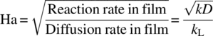
The Hatta number is an important dimensionless number that characterizes the nature of mixing limitations in multiphase mixing‐sensitive reactions. Ha divides multiphase reactions into various regimes. A few of them are described here. A comprehensive description of Ha and its implications in multiphase chemical reaction engineering are described by Doraiswamy and Sharma [11]. For example, Ha < 0.3 means that the bulk phase is saturated and the reaction occurs at the solubility in the bulk phase, as is the case for various gas–liquid (G‐L) or L‐L reactions. On the other hand, Ha > 3 signifies an instantaneous reaction where the entire reaction is completed in the film (or the two reacting components annihilate each other on contact) while only the product is transported across the interphase. Acid–base titrations typically follow this regime. Intermediate reaction regimes are characterized by Ha being between 1 and 3, where part of the reaction occurs in the film while the rest of the reaction happens in the bulk.
For our example, a constant Ha across different reactor scales of operation was desired as a scale‐up factor. To solve the film theory model described in Figure 43.7, ![]() , D, and kLwere estimated from the detailed chemical engineering correlations provided by Baptista et al. [8, 10, 12].
, D, and kLwere estimated from the detailed chemical engineering correlations provided by Baptista et al. [8, 10, 12].
The flux of trifluoromethyl toluene (Ja) was calculated by analytically solving the film diffusion equation. A detailed solution of these equations can be obtained from Baptista et al. [12]. The flux at x = 0 and δ was estimated. Using the global mass balance equations, the molar flux of 4‐trifluoromethyl toluene was then evaluated and correlated with the experimental data. The fit of the model with the experimental data is shown in Figure 43.8.

FIGURE 43.8 Agreement between the experimental conversion of 4‐trifluoromethyl toluene and the modeled conversion as a function of different mixing intensities (quantified by Ha).
It should be emphasized that each data point on Figure 43.8 represents a different Ha due to different mixing intensities imparted during each steady state in the experimental CSTR. It is seen that the film theory model predicts the outcome of the CSTR in a reasonable way and can be used to provide guidance on reaction scale‐up.
Using this model, one can now predict the extent on reaction with different levels of turbulent dissipation energy and Ha. The predictions from the film theory model are shown in Figure 43.9.
FIGURE 43.9 (a) Variation of the model‐predicted % reaction conversion in the film as a function of Ha and impeller power input. (b) Requirement of minimum Ha to achieve the desired reaction endpoint of no more than 5% 4‐trifluoromethyl toluene remaining.
In Figure 43.9a, an increase in the impeller power input leads to an increase in the amount of reaction completed in the film. This is due to the increase in Ha with an increase in the average turbulent dissipation energy. Probing deeper into the phenomenological aspect of the impact of Ha to reaction reveals that higher Ha provides for a higher interfacial area for reaction. The increase in interfacial area is obtained by smaller dispersed phase droplets as the impeller pumps in more energy per unit mass into the contacting device. However, from Figure 43.9a, the analysis tells us that initially increasing the impeller stir rate decreases the droplet sizes easily, but it becomes more difficult to reduce them below a certain size due to surface tension effects manifested by the Weber number.
From a manufacturing viewpoint, a favorable reaction endpoint was judged to be less than 5% 4‐trifluoromethyl toluene remaining, due to relative ease of downstream separation versus added impurity generation. In Figure 43.9b, the desired endpoint of the reaction could be achieved if Ha > 2. The requirement of Ha > 2 in processing could be stated as the requirement that almost 80% of reaction should be done in the interphase film (Figure 43.9a). This is achieved by increasing the interfacial area as a result of more intense agitation provided by the impeller or other mixing devices. In summary, from a process parameter viewpoint, the droplet size distribution has to remain identical with reactor scale‐up. This requirement ensures linear scalability of the interfacial area and constant Ha with increasing reaction scale of operation.
43.3.5 Analysis of Flow Patterns
Two flow patterns were evaluated for the nitration reaction scale‐up. Static mixers were used to evaluate PFR geometry, while a stirred reactor setup in CSTR mode was used to evaluate back‐mixed flow. Assuming heat transfer to not be problematic, the reaction behavior was identical in both if a constant interfacial area criterion was met, manifested in mixing intensity. From a heat transfer viewpoint, the highly exothermic chemistry could favor a tubular flow reactor due to higher heat transfer area per unit volume compared with a stirred reactor. The tubular flow reactor geometry, however, was considered more risky due to potential for solids plugging during a prolonged operation of the L‐L‐S reaction. As a result, a 2 L Hastelloy CSTR with a high L/D (2.5 : 1) ratio was chosen for production.
It should be emphasized that even though a decision was to go ahead with the CSTR, from a fundamental viewpoint, there was a greater risk of spatial variation of Ha in a 2 L CSTR compared with a jacketed static mixer due to a higher volume of reacting fluid with the same heat transfer area. This would potentially result in reaction zones that are not as well mixed (with a lower Ha) and could result in non‐predictive scale‐up. One strategy would be to use CFD to simulate the multiphase flow in a 2 L CSTR, map out the droplet size distribution, and recommend an impeller RPM on the requirement of an acceptable dispersed phase droplet size distribution. However, timelines prevented us from doing this analysis. As a result, a laboratory glass CSTR was already available with geometric similarity to the plant CSTR, and a representative experiment was performed at half the production flow rate in the laboratory. A separate film theory analysis on the glass reactor dictated that the impeller RPM should be set at 700 RPM. This experiment provided passing results for reaction endpoint (99% reaction conversion and 0.3% dinitro impurity) and validated the appropriate scale‐up parameter to be a constant Ha.
43.3.6 Production‐scale CSTR System
Success from using the 2 L glass CSTR in the laboratory provided confidence that we could use the CSTR of the same size in the pilot plant. Completion of the reaction campaign in a reasonable time required removal of 1.5 kW of heat from the CSTR during steady‐state operation. As a result, appropriate chilling capabilities were enabled such that during steady‐state operation, the jacket was kept at 15 °C while the internal temperature was constant at 33 °C. The 2 L CSTR was able to handle the slurry mixture generated in the reaction with constant operation. One campaign with 50 kg production was enabled through this analysis and technology. The product from the CSTR was 98% converted with 0.5% dinitrated impurity, which was much lower than the nearly 4% levels seen during fed‐batch reaction scale‐up to 1 kg. Subsequently, this technology was transferred to the manufacturing site, and more than 200 kg production has been enabled, thereby reducing process safety concerns while delivering consistently high quality and yield of the desired nitrated product.
43.3.7 Conclusions
The application of principles of chemical reaction engineering via the process modeling roadmap enabled a rigorous evaluation of transport phenomena in a multiphase mixing‐limited nitration reaction. Modeling enabled identification of appropriate scale‐up parameters (Hatta number) and ensured that the reaction was scaled up in a safe manner with respect to the exotherm and minimization of the dinitro impurity. This enabled an easier technology transfer to the manufacturing site.
43.4 KINETIC JUSTIFICATION‐BASED CONTROL FOR POTENTIAL MUTAGENIC IMPURITIES
43.4.1 Introduction
Catalytic heterogeneous hydrogenations are one of the most important classes of chemical reactions scaled up in the pharmaceutical industry. These reactions are typically of G‐L‐S type, and a keen knowledge of kinetics and mass transfer is required to ensure proper scale‐up. An added complexity in the specific case of nitro reduction is the high exotherm of such reactions and the potential to form mutagenic impurities that require a strict and an elaborate control strategy for the generation and purge of the same [13]. This example details the application of the process modeling roadmap to understand the kinetics of generation of mutagenic impurities during the nitro reduction step in a late‐stage small molecule compound.
43.4.2 Generation of Mutagenic Impurities During Catalytic Nitro Reduction
The intermediate step involves the heterogeneous catalytic hydrogenation of dinitro core to the corresponding diamino core using a bimetallic catalyst. This is an exothermic reaction, and a fed‐batch process was chosen to conduct the chemistry. The fed‐batch hydrogenation reaction was performed in solvent, while hydrogen gas is supplied to maintain a constant overall hydrogen pressure. This ensures a constant solubility of hydrogen in the reacting solvent. Moreover, earlier studies have shown that the rate of dosing at scale ensured that the reaction had a Hatta number (Ha) < 0.3, which meant the hydrogenation intrinsic kinetics was rate limiting.
Aryl nitro hydrogenations proceed via two monomeric intermediates: an aryl nitroso compound and an aryl hydroxylamine. The presence of the two nitro groups in dinitro pro‐core means that at least eight intermediates are possible along the reaction pathway as shown in Figure 43.10.

FIGURE 43.10 Dinitro pro‐core reduction pathway during catalytic hydrogenation.
In silico evaluation identified the aryl nitro, aryl nitroso, and aryl hydroxylamine substructures as alerts for potential mutagenicity. Since many of the reaction intermediates are unstable, analytical standards could not be prepared, and the mutagenicity of the reaction intermediates could not be determined. A kinetic justification strategy was required to ensure that each hydrogenation intermediate will not be present in diamino core above 1 ppm at the end of hydrogenation reaction process. This was a conservative criterion more than 100‐fold below the Threshold of Toxicological Concern (TTC) in the API.
As a result, a multistep kinetic analysis was required to understand the multivariate interactions, leading to the prediction of such mutagenic impurities with change in process parameters.
To allow for the observation of transient reaction intermediates to develop the kinetic justification, semi‐batch hydrogenation experiments were performed under multivariate conditions that significantly retard the rate of hydrogenation in comparison to the commercial manufacturing process. Further experiments were conducted to prove that the reaction rate was sufficiently slowed by running at a lower temperature and hydrogen pressure, using less catalyst, and running more dilute using additional solvent. These conditions are collectively referred to as the “lowest rate process.” A comparison between the process parameters used in “nominal process” and the “lowest rate process” is shown in Table 43.2.
TABLE 43.2 Comparison Between the Nominal Hydrogenation Conditions (Labeled “Nominal Process”) and the “Lowest Rate Process”
| Parameter | Nominal Process | Lowest Rate Process |
| Temperature (°C) | 70 | 60 |
| H2 pressure (bar absolute) | 2.9 | 2.0 |
| Catalyst loading (kg cat/kg dinitro core) | 0.063 | 0.042 |
| kg solvent 1/kg dinitro core | 8.5 | 10.2 |
Under the “lowest rate process” conditions, the dinitro core is quickly consumed, and three out of the eight possible intermediates (Figure 43.10) along the hydrogenation pathway were detected by anaerobic sampling of the reaction and HPLC analysis. Of these three intermediates, the “NO─NH2” species was fleetingly observed at trace levels before becoming undetectable. The remaining two detectable intermediates, “NHOH─NHOH” and “NHOH─NH2,” and the diamino core (“NH2─NH2”) were used to develop an operational kinetic model and determine kinetic rate constants (k's) using DynoChem software. The reactions included in the kinetic model are listed in Table 43.3.
TABLE 43.3 Data Fitting for the Most Prevalent Intermediates Under the “Lowest Rate Process” Conditions
| Step | Reaction | Parametera |
| 1 | NO2─core─NO2 + * → NHOH─coreNHOH + * | k1 = 2.56 ± 0.23 L/mol s |
| 2 | NHOH─core─NHOH + * → NHOH─core─NH2 + * | k2 = 1.57 ± 0.05 L/mol s |
| 3 | NHOH─core─NH2 + * → NH2‐─core─NH2 + * | k3 = 1.06 ± 0.03 L/mol s |
| 4 | NH2─core─NH2 + * ↔ NH2─core─NH2* | k4 = 1 × 10⁴ L/mol sb k4 = 15.31 ± 0.88 L/mol |
aThe rate constants are reported at 60 °C. The ± values represent the standard error obtained from the DynoChem fitting of the data to the kinetic model (95% confidence interval can be obtained by multiplying the standard error values by 1.96).
bThe rate of adsorption of the diamino core to the catalyst surface (k4) was set to 1 × 10⁴ L/mol s based upon the assumption that adsorption to catalyst surface is very fast. This assumption is implicitly utilized in Eqs. (43.1)–(43.3) as reactive species must absorb to the surface prior to reaction.
The “*” in the reaction steps correspond to a catalytic site. The number of catalytic sites was assumed to be proportional to the total weight loading of catalyst as determined by the vendor. Step 4 in Table 43.3 was added to the model to account for possible catalyst inhibition by the diamino core (“NH2─NH2”). To test for catalyst inhibition, experiments were conducted at the “lowest rate process” conditions with the diamino core charged into the reactor before beginning the reaction. Figure 43.11 shows that as the charged equivalents of the diamino core increased from 0 to 1, the conversion rate of NHOH─NH2 decreased. In other words, the time required to achieve NMT 1 ppm of the reaction intermediates is dependent on the diamino core concentration.
FIGURE 43.11 Comparison of the concentration profile of NHOH─NH2 as a function of the equivalents of the diamino core, NH2─NH2, charged into the reactor prior to start of the reaction. Dashed lines represent calculated values based on the kinetic model.
The concentration vs. time profiles for “NHOH─NHOH,” “NHOH─NH2,” and “NH2─NH2” are shown in Figure 43.12 (no additional “NH2─NH2”) and Figure 43.13 (1 equiv “NH2─NH2”). The dinitro core is the most quickly consumed reaction species (k1 is greater than k2 and k3) and is not shown in Figures 43.12 and 43.13 for clarity.

FIGURE 43.12 Concentration profile of “NHOH─NHOH,” “NHOH─NH2,” and “NH2─NH2” species under the “lowest rate process” conditions. Dashed lines represent calculated values based on the kinetic model.

FIGURE 43.13 Concentration profile of “NHOH─NHOH,” “NHOH─NH2,” and “NH2─NH2” species under the “lowest rate process” conditions with 1 equiv of NH2─NH2 charged at the beginning of the reaction. Dashed lines represent calculated values based on the kinetic model.
The kinetic model accounts for the inhibition caused by the diamino core and predicts the experimental data well. Based upon the kinetic model, the predicted amount of time required for the reaction operating under the “lowest rate process” conditions to reach NMT 1 ppm of potentially mutagenic intermediates is 6.1 hours.
43.4.3 Analysis of Transport Phenomena
The kinetic justification hold time relies on reaction intermediate conversions taking place in a hydrogen‐rich environment (i.e. rate of hydrogen supply to the liquid phase is greater than the rate of hydrogen demand from reaction, Ha < 0.3). The batch must be operated at or above an agitation rate that can achieve a minimum hydrogen interphase mass transfer coefficient of 0.011 s−1. A minimum G‐L mass transfer coefficient (kLa) is specified for nominal hydrogenation process based on the conservative assumptions:
- The overall reaction rate is always limited by G‐L mass transfer (i.e. the intrinsic chemical conversion rate would be significantly higher if not restricted by slow delivery of gas into solution), and, therefore, the rate of reaction is equal to the G‐L mass transfer rate.
- Delivery of stoichiometric amount of hydrogen into solution is accomplished within a 2‐hour period.
Based upon these two boundary conditions and assumptions, 0.011 s−1 was the calculated minimum requirement for kLa for the nominal hydrogenation process. The minimum kLa was determined in this manner:
where
- [A*] is the equilibrium solubility of H2 in 2‐methyltetrahydrofuran (2‐MeTHF) determined at 2 barg H2 and 70 °C = 0.007 25 mol H2/L (from DynoChem – H2 solubility and heat of reaction utility)
- [At] is the concentration of H2 on catalyst surface = 0 mol H2/L (mass transfer limited)
- From DynoChem simulations, R required = 7.839 × 10⁻⁵ mol/(L s):
The kLa measurement was carried out in the commercial equipment using the primary process solvent at a volume equal to the final batch volume.
As an additional level of assurance that the process is not G‐L mass transfer limited, a mass transfer hold of 4 hours, twice the 2‐hour period stipulated above, was used to ensure that potentially mutagenic intermediates are consumed even when operating at the lower limit of the kLa. This mass transfer hold time under hydrogenation conditions is followed by the reaction kinetics control hold time of 12 hours. Thus, the total reaction hold time is 16 hours, which is the sum of the mass transfer and reaction kinetics hold times. A 16‐hour hold time under the nominal hydrogenation conditions provides multiple layers of assurance that the reaction intermediates will be NMT 1 ppm in the hydrogenation.
43.4.4 Conclusions
An understanding of the kinetics of the reaction pathway observed during catalytic hydrogenation was required to ensure process robustness with respect to the purge of the mutagenic impurities that can potentially appear in the API. This was accomplished by building a multivariate kinetic model coupled with an analysis of the G‐L mass transfer of hydrogen under worst‐case scenarios. The model recommendations were supplemented with mass transfer experiments performed at the manufacturing‐scale reactors. This multivariate understanding of reaction kinetics and the transport phenomena provided a control strategy to limit the amount of mutagenic impurity at the end of the hydrogenation process for a late‐stage compound.
ACKNOWLEDGMENTS
This work was sponsored by AbbVie. AbbVie contributed to the design, research, and interpretation of data, writing, reviewing, and approving the publication. Anuj Verma, Steven Richter, Brian Kotecki, and Moiz Diwan are employees of AbbVie. The authors would like to thank Niharika Chauhan, Samrat Mukherjee, Kaid Harper, Benoit‐Cardinal David, Shailendra Bordawekar, and Nandkishor Nere for providing experimental results and helpful comments.
LIST OF SYMBOLS
| P | total pressure |
| T | temperature |
| τ | space time |
| Da | Damköhler number |
| ν | kinematic viscosity |
| ε | dissipation rate of turbulent kinetic energy |
| Λc | mesomixing length scale |
| QB | reagent dose rate |
| Apipe | cross‐sectional area of feed pipe |
| u | velocity of surrounding fluid in reactor |
| <T> | average temperature of the surrounding fluid |
| [Ai] | concentration in test volume/within the film |
| <[Ai]> | average concentration of active species in the surrounding fluid |
| <u> | average velocity of the surrounding fluid in reactor |
| Δρ | density difference |
| δ | film thickness |
| molar flow rate of component A entering the organic phase | |
| molar flow rate of component A exiting the organic phase | |
| [Aorg] | concentration of A in the well‐mixed organic phase |
| JA|x=0 | flux of A at x = 0 |
| JA|x=δ | flux of A at x = δ |
| molar flow rate of component A exiting the aqueous phase | |
| interfacial area | |
| V | volume of phase |
| εa | holdup fraction |
| k | pseudo‐first‐order rate constant |
| D | diffusivity |
| Ha | Hatta number |
| kL | mass transfer coefficient |
| [A*] | solubility/equilibrium concentration |
REFERENCES
- 1. Bird, R.B., Stewart, W.E., and Lightfoot, E.N. (2002). Transport Phenomena. Hoboken, NJ: Wiley.
- 2. Bourne, J.R. (2003). Mixing and the selectivity of chemical reactions. Organic Process Research & Development 7 (4): 471–508.
- 3. Pelleter, J. and Renaud, F. (2009). Facile, fast and safe process development of nitration and bromination reactions using continuous flow reactors. Organic Process Research & Development 13 (4): 698–705.
- 4. Burns, J.R. and Ramshaw, C. (2002). A microreactor for the nitration of benzene and toluene. Chemical Engineering Communications 189 (12): 1611–1628.
- 5. Brocklehurst, C.E., Lehmann, H., and La Vecchia, L. (2011). Nitration chemistry in continuous flow using fuming nitric acid in a commercially available flow reactor. Organic Process Research & Development 15 (6): 1447–1453.
- 6. Hartman, R.L., McMullen, J.P., and Jensen, K.F. (2011). Deciding whether to go with the flow: evaluating the merits of flow reactors for synthesis. Angewandte Chemie International Edition 50 (33): 7502–7519.
- 7. Kulkarni, A.A., Kalyani, V.S., Joshi, R.A., and Joshi, R.R. (2009). Continuous flow nitration of benzaldehyde. Organic Process Research & Development 13 (5): 999–1002.
- 8. Quadros, P.A., Oliveira, N.M.C., and Baptista, C.M.S.G. (2005). Continuous adiabatic industrial benzene nitration with mixed acid at a pilot plant scale. Chemical Engineering Journal 108 (1–2): 1–11.
- 9. Esteves, P.M., de M. Carneiro, J.W., Cardoso, S.P. et al. (2003). Unified mechanistic concept of electrophilic aromatic nitration: convergence of computational results and experimental data. Journal of the American Chemical Society 125 (16): 4836–4849.
- 10. Quadros, P.A., Reis, M.S., and Baptista, C.M.S.G. (2005). Different modeling approaches for a heterogeneous liquid−liquid reaction process. Industrial & Engineering Chemistry Research 44 (25): 9414–9421.
- 11. Doraiswamy, L.K. and Sharma, M.M. (1984). Heterogeneous Reactions: Analysis, Examples, and Reactor Design. 2. Fluid‐fluid‐solid Reactions. New York: Wiley.
- 12. Quadros, P.A., Oliveira, N.M.C., and Baptista, C.M.S.G. (2004). Benzene nitration: validation of heterogeneous reaction models. Chemical Engineering Science 59 (22–23): 5449–5454.
- 13. Betori, R.C., Kallemeyn, J.M., and Welch, D.S. (2015). A kinetics‐based approach for the assignment of reactivity purge factors. Organic Process Research & Development 19 (11): 1517–1523.