
17
CHEMICAL ENGINEERING PRINCIPLES IN BIOLOGICS: UNIQUE CHALLENGES AND APPLICATIONS
Sourav Kundu and Vivek Bhatnagar
Biologics R&D, Teva Pharmaceuticals, Inc., West Chester, PA, USA
Naveen Pathak
Process Development and Technical Services, Shire plc, Cambridge, MA, USA
Cenk Undey
Process Development, Amgen Inc., Thousand Oaks, CA, USA
Therapeutic proteins now represent a major class of pharmaceuticals. These macromolecules, generally referred to as biologics, are either natural (e.g. protein fractions from donor human plasma) or are commonly made in bacterial or mammalian host systems by recombinant DNA technology. In the case of the latter, through modern molecular biology techniques, genes representing human proteins, protein fragments, or antibodies to therapeutic targets can be inserted into a host system such as the bacterium Escherichia coli or a mammalian host cell such as Chinese hamster ovary (CHO) cells. The host cells are then grown in fermenters or bioreactors using nutrient‐rich media and highly controlled conditions. The host cells are internally programmed to synthesize the protein of interest. The synthesized protein may reside in high concentrations within the cell in inclusion bodies or secreted into the extracellular environment. The protein then can be harvested in large quantities and purified to the final therapeutic dosage form. This is of course an oversimplification of a very complex biological production process that brings a protein therapeutic to patients.
Chemical engineering principles apply widely in development and production of biologics. During discovery, biologic drugs are first made in the laboratory in small scale (less than a milliliter to a few liters), quantities sufficient for testing in vitro or in an animal model. As the feasibility is proven, the process is refined and scaled up to manufacture quantities needed for extensive pharmacological, toxicological, and clinical testing. At this stage, the culture volume is typically increased to a few hundred to a few thousand liters. After the clinical safety and efficacy are proven and regulatory approval for commercialization is obtained, the drug may be manufactured at even larger scale such as 10–20 000 L. At each of these stages of product development life cycle, chemical engineering principles such as mass transfer, heat transfer, fluid mechanics, chemical reaction kinetics, etc. are used. As the production process is scaled up during the product development, many of the process characteristics defined by dimensionless numbers widely used in chemical engineering (e.g. Reynolds number, Nusselt number, Newton number [also known as Power number], etc.) are kept similar between scales. In fact, many of these dimensionless numbers provide the basis for scale continuum that is extremely important for consistency and comparability.
In the cell culture process for mammalian systems, chemical engineering principles are used to optimize transport of nutrients, supply of oxygen to the cells, and facilitate mixing for homogeneity, removal of undesired metabolites and toxins, and collection of the protein of interest. In the downstream purification process, chemical engineering principles are used for separation of the protein drug from associated impurities, concentration of the protein drug, removal of undesired microorganisms, and stabilization of the protein drug to a state appropriate for storage, transport, and administration. Later in the chapter we will describe in greater detail various unit operations that are typically involved in production of biologics and the specific fundamental principles associated with these unit operations.
17.1 WHY ARE BIOLOGICS UNIQUE FROM A MASS, HEAT, AND MOMENTUM TRANSFER STANDPOINT?
In order to fully appreciate why biologics are unique, it is important to discuss the complexity of the structure of these macromolecules. As stated earlier, biologics are protein molecules of therapeutic value most commonly administered as aqueous solution. The molecular weight of these macromolecules can range from 5–30 kDa (e.g. recombinant insulin, molecular weight ~6 kDa; recombinant human growth hormone, molecular weight ~22 kDa; etc.) to hundreds of kDa (e.g. recombinant factor VIII, molecular weight ~280 kDa). More complex and larger macromolecules are also being produced in recombinant forms such as recombinant von Willebrand factor, which is made as a functional multimer with an approximate molecular weight reaching in the millions of daltons. Monoclonal antibodies represent an important class of protein drugs. Chimeric or humanized recombinant monoclonal antibodies have found wide applications as receptor blockers, receptor stimulators, delivery vehicles, or absorbents for undesirable antigens in various therapeutic, diagnostic, or imaging areas.
Protein molecules are composed of amino acid sequences determined by the genetic code residing in the DNA. Protein synthesis takes place on ribosomes. The amino acids are connected to each other by peptide bonds, forming polypeptide chains that provide the backbone of a protein molecule. Additional cross‐links may be formed within a polypeptide chain or between adjacent branches of polypeptide chains through the disulfide bridges, creating complex folds and a three‐dimensional geometry. Protein architecture comprises four levels of structure. The primary structure describes the amino acid sequence and the location of any disulfide bridges within the polypeptide chain and branches. The secondary structure describes the spatial arrangement of neighboring amino acids within the linear sequence. The tertiary structure of a protein describes the spatial arrangement of amino acids that are far apart in the linear sequence. If the protein molecule contains more than one polypeptide chain (also called the subunits), the spatial arrangement of these subunits are described in the quaternary structure. Additional complexity may arise when polypeptide chains fold into two or more compact globular regions joined by flexible portions. These domains resemble each other at times and vary in function at other times [1].
In addition to the characteristic three‐dimensional peptide structures, many protein macromolecules also have covalently linked carbohydrate branches. These are known as glycoproteins and represent an important class of therapeutic molecules. The carbohydrate structure takes its initial shape in the endoplasmic reticulum during synthesis and modified into its final form in the Golgi complex. The carbohydrates (also known as oligosaccharides) can be linked to the polypeptide chain of the glycoprotein through the side‐chain oxygen atom on the amino acids serine or threonine residues by O‐glycosidic linkages or to the side‐chain nitrogen of asparagine residues by N‐glycosidic linkages. In addition to these carbohydrate cores, there can be other polysaccharides attached to these cores in a variety of configuration causing a diverse and defining carbohydrate structure [1].
The three‐dimensional structure of a protein is extremely important for its functionality. Many interactions between protein molecules or between a protein molecule and a receptor on a cell require a specific spatial geometry of the polypeptide chain. Any disturbance in the three‐dimensional structure bears the risk of loss of the protein's biological activity, bioavailability, or its therapeutic value. Environmental conditions that can alter the three‐dimensional structure include pH, temperature, physical forces such as shear, specific concentration of chemicals such as chaotropic agents (chemicals that disrupt the protein three‐dimensional structure such as urea or guanidine hydrochloride at high concentrations) and organic solvents, etc. The alteration of structure can be reversible and can actually be used for recovery of proteins. For example, highly aggregated recombinant protein housed in the inclusion bodies of E. coli can be solubilized in high concentration of urea or guanidine hydrochloride followed by a controlled removal of the chemicals. The process allows the protein to disaggregate and refold into its native desirable state. Under certain conditions the alteration of structure becomes irreversible. The common environmental conditions causing permanent structural alteration of a protein are exposure to extreme heat, pH, or chemical concentration. In response to environmental conditions, such as heat, protein unfolds into a denatured state from its native state. Subsequent aggregation of the denatured molecules results in irreversible denaturation. Denaturation and aggregation during processing are of particular concern to a manufacturer of biologics. Thermal denaturation and unfolding of proteins can be studied by using differential scanning calorimetry (DSC) where heat flux is measured in a sample as the temperature is gradually increased. The protein sample provides a characteristic curve representative of glass transition and phase changes. Denaturation of a protein drug can lead to the loss of its biological activity. In one study [2], natural and recombinant Protein C evaluated by DSC was observed to undergo rapid decline in activity as temperature was increased from 20 °C with a complete loss of activity at temperatures above 70 °C. Narhi et al. observed irreversible thermal unfolding of recombinant human megakaryocyte growth factor upon heating, leading to formation of soluble aggregates ranging in size from tetramer to 14‐mer [3]. Proteins can be affected by cold temperatures as well. Protein solutions may be exposed to temperatures lower than −50 °C during freeze‐drying in order to prepare a protein drug dosage form. Although less concerning than heat‐induced structural damage, cold inactivation has been seen with enzymes such as phosphofructokinase [4] or with proteins such as β‐lactoglobulin [5].
In addition to loss of biological activity, when administered to a patient, the structural change from the native state can trigger adverse cellular and immunological response, causing serious medical consequence. Therefore, manufacturing processes for biologic drugs are designed to have appropriate controls such that the protein's active state is maintained. The likelihood of irreversible denaturation is high during operations involving elevated temperature, contact with excessively high or low pH, vigorous fluid movement (e.g. vortex formation), or contact with air interface (e.g. foaming). Thermal denaturation can occur during processing if the temperature is not maintained at the facility or the equipment level or if unintended local heat buildup occurs in the processing equipment such as in a rotary lobe pump, a commonly used component of a bioprocess skid. Most biopharmaceutical plants have sophisticated environmental controls with high‐efficiency HVAC systems to maintain the ambient temperature at a level that is far away from the denaturation temperature of the protein. Temperature is also controlled at the equipment level through water or ethylene glycol heat exchange fluids circulating through the jacket of a process vessel. When heating of a chilled protein solution (typically in between process steps) is needed, the jacket temperature is capped at 45–50 °C to prevent excessive vessel skin temperature that may cause denaturation. Exposure to excessively high or low pH can occur during titration of a protein solution with acid or alkali during processing. It can be avoided by ensuring rapid mixing in the vessel through appropriately designed agitators, by controlling the flow rate of the reagents, and by using lower titrant concentrations.
Appropriate handling of a protein solution during processing is extremely important. Abrupt and vigorous fluid movement such as those encountered during movement of tanks during shipping of liquid protein solutions can be detrimental and result in denaturation. Air entrapment and exposure of protein to an air interface create the bulk of the problem in these cases [6]. Process equipment and piping are designed such that the protein solution is not subjected to highly turbulent flow regions during transport. Effect of shear on proteins remains a controversial topic. Thomas provides an excellent overview of the issue of shear in bioprocessing [7]. While loss of activity has been seen with enzymes when exposed to high shear forces in a viscometer, denaturation of globular proteins is less likely just from high shear fields. As mentioned earlier, the primary mechanism of denaturation appears to be from the gas–liquid interface, especially if high velocity gradients are present. Lower concentration solutions are more susceptible to the damage. Design of equipment to minimize air entrapment (e.g. avoidance of pump cavitation) allows control of inactivation and protein denaturation in bioprocessing.
Cell culture fluids pose unique chemical engineering challenges as well. The cells require oxygen and respire carbon dioxide. Oxygen is sparged into the culture that produces bubbles and foam. Care needs to be taken to control the bubble size, velocity, and amount since the bubbles can carry cells to the surface and cause cell death upon bursting. Other chemical engineering challenges include the heat input (mammalian cells) or removal (microbial cells) requirements, mixing requirement, maintenance of appropriate pH conditions, nutrient delivery, and metabolite removal for large industrial‐scale cell culture systems. Further details of bioreactor design and operation are provided in Section 17.3.1.
The complexity of proteins drugs and their biological production systems pose extraordinary challenges to the chemical engineers with responsibility for industrial‐scale manufacturing of these products. Design, development, and operation of these processes require complete understanding and appreciation for the intricacies of proteins and living cells. In this chapter we will examine how concepts taught in traditional chemical engineering are applied to design equipment and develop processes that allow modern‐day mass manufacture of biotechnology products.
17.2 SCALE‐UP APPROACHES AND ASSOCIATED CHALLENGES IN BIOLOGICS MANUFACTURING
With the introduction of recombinant human insulin by Genentech/Roche (later licensed to Eli Lilly & Co.) in 1978, the commercial industrial biotechnology was born. It was clear that products created by recombinant DNA technology hold an immense potential for curing “uncurable” diseases such as cancer. The biotechnology products no longer were just research tools in the laboratory made in milligram quantities, but they needed to be manufactured in bulk in commercial‐scale manufacturing facilities. Scale‐up and optimization of biologics manufacturing processes rapidly became critical for the success and growth of the industry.
Scale‐up of biologics manufacturing processes utilizes similar engineering principles as scale‐up of chemical manufacturing processes. In the laboratory, the cell culture may be performed in shaker flasks, roller bottles, or small glass stirred tank bioreactors. Flask‐ or bottle‐based cultures can be scaled up by simply increasing the number of flasks or bottles with some increase in the size. Bioreactors can be successfully scaled up linearly from 1 to 25 000 L or above by preserving the aspect ratios, impeller sizing ratios, impeller spacing ratios, and baffle geometries. Design of spargers for oxygen delivery to the cell culture may differ considerably between small‐scale and industrial‐scale bioreactors. While a small sparge stone may be adequate for oxygen delivery in a small‐scale bioreactor, much more elaborate sparging systems with one or more drilled pipes may be necessary to deliver the quantity of oxygen needed in a large‐scale bioreactor. The oxygen concentration is maintained at the same level between the small and large scales by controlling to a specified dissolved oxygen (DO) setting determined during process development and preserved through scale‐up. In order to achieve the level of DO during cell culture, an adequate amount of oxygen is fed to the bioreactor typically through a flow controller. For large‐scale bioreactors, the piping and delivery system for gases can become rather massive. The delivery of oxygen to the cells is dependent on the mass transfer of oxygen from bubbles in the stirred tank to the liquid where the cells are situated. The bubble size is governed by the sparger type and whether the bubbles are broken up further with a Rushton (turbine)‐type impeller at the bottom of the bioreactor. The mass transfer coefficient kLa is an important parameter that determines if adequate transport of oxygen to the cells can be achieved and must be calculated for each bioreactor where scale‐up is being performed. The oxygen uptake rate (OUR) is the oxygen required for the optimum culture performance that must be matched by the oxygen transfer rate (OTR) that is determined by the mass transfer coefficient. The relationship between OUR and OTR at a constant DO level is shown by the following formula:

where
- μ is the specific growth rate.
- X is the measured cell density
-
 is the calculated cell yield per unit oxygen consumption.
 - Csat and CL are the DO concentrations at saturation and at any given time in the liquid phase, respectively.
Scaling up a suspension cell culture requires a thorough evaluation of mixing. Adequate mixing is necessary to deliver nutrients and oxygen to cells, removal of metabolites from the microenvironment, and dispersion of additives such as shear protectants and antifoam. Scale‐up of mixing is often performed by maintaining similar power per unit volume (P/V) between the small‐scale and large‐scale bioreactors. P/V is calculated from the impeller geometry, agitation rate, and working volume of the stirred tank according to the following formula:
where
- ρ is density.
- n is the number of impellers.
- Np is the impeller power number.
- N is the agitation rate.
- Di is the impeller diameter.
- V is the working volume of the tank.
When P/V is preserved during scale‐up, it is expected that with geometric similarity between the small‐ and large‐scale bioreactors, circulation time, mixing time, and impeller tip speed increase, but the size of the eddies do not change, hence ensuring mixing and mass transport [8]. P/V can be reported as an ungassed value or a gassed value. Typically, the measured ungassed value is slightly higher than the measured gassed value as a result of loss of power upon introduction of gas sparging in the bioreactor. Impeller tip speed is determined by the following formula:
Maintaining impeller tip speed between scales can ensure similar shear‐induced damage of cells between scales. It is important to minimize shear‐induced cell damage in order to maintain cell viability and prevent release of unwanted enzymes, host cell DNA, and other impurities into the cell culture. The ability of cells to withstand shear occurring at the tip of the impeller blade is dependent on the type of cells. Typically microbial cells can withstand more shear and therefore can be agitated more aggressively than mammalian cells. It is helpful to scale up in stages when transferring a process from a laboratory to a commercial manufacturing facility. The stepwise approach reduces the probability of failure and allows troubleshooting and understanding of scale‐dependent product quality characteristics that are not uncommon. Beyond mixing, mass transfer, and shear characteristics, insight is needed with respect to bioreactor control parameters such as pH, temperature, DO, dissolved carbon dioxide, overlay pressure, and feed addition requirements for a successful bioreactor scale‐up [8–11].
Scale‐up of the downstream purification steps utilizes similar concepts as the upstream cell culture process. In the scale‐up of the chromatography columns, the bed height and linear flow rate are generally preserved between the small‐scale and large‐scale columns. The volumetric output needed for commercial manufacturing is achieved by increased diameter and bed volume of the large‐scale column. Modern chromatography resins provide high protein loading capacity often exceeding 30 g/L. This helps reduce the total bed volume and size of the column necessary. In addition, modern chromatography resins can withstand higher pressures without getting crushed or deformed. This allows operation of the column at higher flow rates, shortening the overall processing time. Column packing methods may differ significantly between the small columns used in the laboratory and large columns used in a commercial manufacturing facility. The complexity of packing increases significantly in larger columns just because of the size. In addition, column hardware components such as the screen, flow distribution system, and head plate play much more important role in large‐scale columns. Section 17.3.3 in this chapter provides more information on column packing.
Scale‐up of tangential flow filtration (TFF) systems have become easier due to the availability of membrane cassettes of various sizes. For example, Pellicon™ 2 TFF cassettes manufactured by Millipore Corporation (Billerica, MA) are available in 0.1, 0.5, and 2.5 m2 membrane area configurations. Multiple 2.5 m2 cassettes can be stacked together to provide the necessary membrane area for large‐scale ultrafiltration operations. Other manufacturers also offer similar choice of sizes and molecular weight cutoffs to match scale and process needs. TFF can be scaled up by maintaining filtrate volume to membrane surface area ratios the same between laboratory‐scale and commercial‐scale systems. In addition, membrane material, molecular weight cutoff (determines retention characteristics), channel height and flow path type, and retentate and filtrate pressures are kept similar between the two scales [12, 13]. Other considerations for scale‐up of a TFF system include the type of pump used, number of pump passes that the protein solution experiences during the operation, configuration and sizing of the piping, and the process time. Rotary lobe pumps are commonly used in large scale, while a small‐scale TFF operation may be performed with an air‐driven diaphragm pump or a peristaltic pump. The number of pump passes is an important consideration for thermally labile proteins. The retentate protein solution may experience a rise in temperature if the concentration factor is high. Some large‐scale retentate tanks are equipped with cooling jackets to prevent heat buildup and potential denaturation of the protein. The size of the piping and configuration of the flow path in the large‐scale equipment are carefully selected to ensure that excessive pressure drop does not occur or frictional forces do not become too large. Generally these are not major concerns in the laboratory‐scale equipment. It is a good idea to maintain similar process time between the small‐scale and large‐scale systems. This allows for process consistency across scale and ensures predictable product quality during scale‐up.
Microporous membrane filtration is another important type of unit operation employed in biopharmaceutical manufacturing. Hollow fiber cartridges can be used to produce filtrate in microfiltration. In this case linear scaling can be readily accomplished by keeping the fiber length similar between scales. The size of the fiber bundle may increase depending on the volume of material to be processed.
Other unit operations that are typically used for bioprocessing are normal flow filtration (NFF), centrifugation, and various types of mixing. While we will not discuss scale‐up of each one separately, it is clear from the discussion so far that similar approaches utilizing basic principles of chemical engineering can be successfully used in all of these cases.
17.3 CHALLENGES IN LARGE‐SCALE PROTEIN MANUFACTURING
Large‐scale protein manufacturing utilizes a series of unit operations to grow cells, produce product, and isolate and purify product from the cell culture. In the following sections, we will examine these steps in more detail and discuss chemical engineering challenges associated with these steps.
17.3.1 Bioreactor
A bioreactor provides a well‐controlled artificial environment to the protein‐producing host cells that promote cell growth and product synthesis. Bioprocesses have multiple seed bioreactor steps to sequentially increase culture volume that finally culminates in a production bioreactor where product expression occurs. The design criteria for production bioreactor and the seed bioreactors could differ substantially as the goals in the two systems are different. However, the concepts presented here are applicable for either system.
Mammalian cells lack an outer cell wall and are sensitive to shear forces and damage by bursting bubbles. Lack of a cell wall directly exposes a cell's plasma membrane to environmental stresses. Plasma membrane contains enzymes and structural proteins that play a key role in the communication between cell and its environment [14]. Microbial cells are enveloped by a cell wall that imparts much higher tolerance to shear. Growth rates for the microorganisms are also much higher. Thus, the design criteria for fermenters are geared toward providing adequate nutrients to the culture and less concerned with the shear introduced through agitation. Due to these conflicting requirements, very few dual‐purpose vessels designed for both mammalian and microbial cell cultivation are in use.
Environmental conditions in the bioreactor such as osmolality, pH, and nutrient concentrations could significantly affect quantity of protein expressed as well as product quality attributes. By product quality attributes we mean properties of the protein in terms of its structure, function, and stability. Complexity of maintaining live cells under optimal conditions dictates the design of the bioreactors. Over the years different designs of bioreactors have been developed. Most common is the stirred tank system, which is widely used for free suspension cell culture. Other designs that are also used commercially are hollow fiber bioreactors, air‐lift bioreactors, and, more recently developed, various types of disposable plastic bag‐based bioreactors. Each design provides some advantages as well as unique challenges. We will limit the scope of this discussion to the stirred tank bioreactor system.
Stirred tank bioreactors have emerged as a clear winner in the twenty‐first century for culturing mammalian cells. One of the key reasons is that the mammalian cells have proved to be sturdier than initially thought of [15]. Stirred tank bioreactors are available in the widest capacity range (1 –30 000 L) and commercially used in cultivating different cell lines (e.g. CHO, MDCK, BHK, NS/0, etc.). Fermenters used in commercial microbial and yeast fermentation processes are also primarily stirred tank vessels. Fermentation processes have been successfully scaled up to 250 000 L capacity.
Bioreactor and fermenter systems operate under aseptic conditions, which require exclusion of undesired contaminating organisms. Bioreactors and associated piping are designed as pressure vessels such that these can withstand heat sterilization with saturated steam. All entry points to the vessel for adding and removing gases or liquids are designed to maintain aseptic conditions. The requirement for aseptic processing and heat sterilization of the system is specific to bioprocesses. Factors that determine success of any sterilization regimen are exposure time, temperature, and system conditions. Equipment is designed to avoid buildup of condensate that forms as the saturated steam transfers heat to the vessel interior or to the piping. Buildup of condensate can cause “cold spots,” resulting in insufficient microorganism “kill” and failed sterilization. Piping connected to the bioreactor is equipped with steam traps to ensure aseptic removal of the condensate. Exposure to saturated steam causes coagulation of proteins in the microorganisms, rendering them nonviable. The thermal death of microorganisms is a first‐order process [16] and can be described by the following equation:
where
- Cv is the concentration of viable microorganisms.
- t is the time.
- k is the thermal death rate constant.
Integration of this equation from a time 0 (t0) when the viable microorganism concentration is Cv0 to a finite time t provides the following expression:
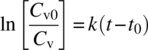
The equation can be used to calculate the time required to achieve a log reduction of microorganisms when the thermal death rate constant for a type of microorganism is known.
Bioreactor operation can be considered to be a two‐step chemical reaction. The first step is the cell growth and the final step is product synthesis by the cells. For growth‐associated products such as monoclonal antibodies, the two steps are not mutually exclusive and thus have to be considered as concurrent reactions. Protein expressed from genetically engineered mammalian cells is constitutive, i.e. protein expression is independent of the growth phase of the culture. For non‐growth‐associated products like expression of viral antigens, the two steps could be treated as different phases and may even require different operating conditions such as temperature shifts, pH shifts, etc. Induction or infection of the culture for expression of these non‐growth‐associated products may even trigger cell destruction, e.g. seen in production of interferons. Similar to the chemical reaction kinetics, stoichiometric and kinetic equations for cell growth and product formation have been developed [17]. Modern laboratory systems are used to determine concentrations of cells, nutrients, metabolites, and product at different stages of the process. These key experimental data generated in the laboratory are used to develop temporal correlations for cell growth, nutrient uptake, and product synthesis. These correlations are used to calculate kinetic parameters such as specific growth rates or specific nutrient uptake rate. Table 17.1 lists the typical cell culture parameters related to growth and product formation along with their definitions.
TABLE 17.1 Parameters Commonly Used for Measurement of Cell Culture Growth and Product Formation
| Parameter | Definition | Unit | Mathematical Expression |
| Growth rate (G) | Rate of change in number of cells | No. of cells/L‐h | x, viable cell density (cells/mL) at time t |
| Specific growth rate | Normalized growth rate | h−1 | |
| Specific nutrient consumption rate | Normalized uptake rate of a nutrient (e.g. glucose, glutamine, oxygen, etc.) | g nutrient/g cell‐h | s, nutrient concentration |
| Specific product formation rate | Normalized rate of product synthesis | g product/g cell‐h | p, product concentration |
| Specific lactate formation | Lactate formed per unit glucose consumed | g lactate produced/g glucose consumed | [lac], lactate concentration [glu], glucose concentration |
For other design aspects of a bioreactor, most chemical engineering principles for chemical reactor design remain applicable. Chemical engineers play an important role in establishing the design criteria for the bioreactors. These design criteria are established with the goal of providing the organism with optimal conditions for product synthesis. To prevent formation of localized environment, homogeneous mixing of the culture is essential. Further, transfer of oxygen to the culture and removal of carbon dioxide from the system have to be achieved. The critical role for the process engineer is the identification of the design criteria that can meet these requirements. The process engineer analyzes the data generated in the laboratory using small‐scale bioreactors and identifies key process operating parameters and their appropriate settings. These often include pH, DO, agitator speed, dissolved carbon dioxide, and initial viable cell density (VCD). The set points and normal ranges of these operating parameters are selected such that consistent and acceptable quality of the protein can be obtained run after run. Typically the cell culture is optimized to yield the highest product concentration, commonly called titer. However, in many instances, as more titer is obtained from the culture, the amount of unwanted impurities such as fragmented or misfolded proteins, host cell DNA, and cellular proteins, cell debris, etc. starts to increase. Therefore, a careful balance has to be achieved between titer and amount of impurities. The capacity of the downstream purification steps for impurity removal is a major consideration. If the downstream steps are capable of removing large quantities of impurities coming from the production bioreactor, the cell culture can be forced to produce high titers accompanied by higher amounts of impurities that can be reproducibly cleared. During process development, process is scaled up from a small‐scale to an intermediate‐scale pilot laboratory bioreactor operated at the same set points as the small‐scale bioreactor. Acceptable quality of the pilot‐scale material confirms the validity of the scale‐up. If successful, then the same criteria are used to scale up to the commercial‐scale bioreactors. Otherwise, further characterization work is undertaken to better understand the cell culture process requirements and the process fit to the equipment, and the cycle is repeated.
Key characteristics of stirred tank bioreactors used for production of therapeutic protein molecules are described in the following subsections.
17.3.1.1 Vessel Geometry
The tanks used for mammalian cell culture were “short and fat.” Original bioreactor systems had an aspect ratio of vessel height to inside diameter of 1 : 1. This geometry allows proper mixing at low agitation speed. Currently, use of an aspect ratio of 2 : 1 is widely accepted, while use of tanks with 3 : 1 aspect ratio has also been reported. Matching aspect ratios between the bench‐scale and the commercial‐scale bioreactors facilitates process scale‐up but is seldom used as a strict scale‐up criterion. Lower aspect ratio for small‐scale bioreactors is acceptable, but for large‐scale bioreactors lower aspect ratio creates a larger footprint that becomes cost prohibitive to implement. Figure 17.1 shows a simplified schematic diagram of a bioreactor showing important internal components of the vessel. There are many possible variations for the configurations of the impellers, sparger assembly, and the baffle system.

FIGURE 17.1 A simplistic schematic diagram of a cell culture bioreactor showing internal components. Many variations of sparge tube, impeller, and baffle configuration are possible.
17.3.1.2 Mechanical Agitation
Gentle mixing in the bioreactor is essential to maintain homogeneity, facilitate mass transfer, and support heat transfer. Three‐blade down‐pumping axial flow impellers are the most common design used in bioreactors. Number of impellers used is governed by the aspect ratio of the vessel. A bioreactor with an aspect ratio of 2 : 1 is typically equipped with two axial flow impellers of diameter equal to one‐half of the tank diameter. If the impellers are too closely placed, then maximum power transfer is not achieved. For optimal results, space between the two impellers is between one and two impeller diameters. Actual placement of the impeller within this range is also governed by the operating volume in the tank so as to avoid the liquid levels where the rotating impeller is not fully immersed (also known as “splash zone”) and may entrap air, causing unnecessary and detrimental foaming.
Commercial‐scale bioreactors have bottom mount drives. This is preferred because it allows for a relatively shorter shaft. A shorter shaft provides structural integrity and absence of wobbling when the agitator is running. Removing the impellers for maintenance becomes easier with a bottom mount impeller system. In addition, head room requirement within the production suite is also less compared to a top mount drive for which sufficient ceiling height is required to be able to remove the impeller without having to open the ceiling hatch and exposing the bioreactor suite to the outside environment. Shaft seal design for a bottom mount drive bioreactor poses significant challenges. Typically, a double mechanical seal is used that is constantly lubricated by clean steam condensate fed to the seal interface, and a differential pressure is maintained across the seal so that bioreactor fluid does not enter the seal space, reducing possibility of contamination. For smaller‐sized seed bioreactors, a top mount drive could be considered to eliminate mechanical seal design issues. Design of the seal is often not given the same level of attention as some of the other parts of the system. Apart from the absolute requirement of maintaining aseptic conditions, the ease of maintenance of the seal should also be considered.
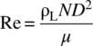
The Reynolds number (Re) in a bioreactor is expressed by the following equation:
where
- ρL is the density of the media (kg/m3).
- μ is the viscosity of the media (Pa∙s).
- D is the impeller diameter (m).
- N is the impeller speed (revolution/second).
The viscosity of the cell culture fluid is close to that of water. Thus, Reynolds number > 104 is often experienced in the bioreactor, which allows utilization of turbulent flow theories to analyze the fluid mechanics in the bioreactor.
17.3.1.3 Mass Transfer
Rate of oxygen transfer to the liquid in a bioreactor is governed by the difference between the oxygen concentration in the gas phase and the concentration of oxygen in the liquid culture, fluid properties, and the contact area between the gas and the liquid. Pressurized air–oxygen mixture is supplied to the sparger, which is either a ring or a tube with open end or with holes on the sidewall. Two spargers may be required in a production bioreactor, while the seed bioreactors may have only one sparger. The size of the bubbles and their distribution are key to the efficiency of mass transfer to the liquid. For a given air–oxygen mix, the higher the concentration of DO levels in the cell culture fluid, the lower the efficiency of oxygen transfer to the fluid as the concentration difference is the driving force. To increase mass transfer in the existing equipment, composition of the gas (oxygen enrichment) may be altered, or the gas flow rate may be increased. Higher sparge gas flows result in increased carbon dioxide stripping [5]. Thus, as a result of the selected strategy, carbon dioxide levels in the culture may vary. Above a certain concentration (usually partial pressure of >140 mmHg), carbon dioxide has a toxic effect on the cell culture, resulting in product quality issues. Therefore, careful control of carbon dioxide concentration in the culture is essential for cell health and product quality.
Respiratory quotient (RQ) is defined as the rate of carbon dioxide formation divided by the rate of oxygen consumption. RQ for mammalian cells is close to 1.0. This implies that for each mole of oxygen consumed, one mole of carbon dioxide is produced. Generally, bioreactors are maintained at DO levels of greater than 30%.
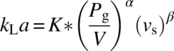
In the steady state, the OTR from the gas bubbles to the cells is matched by the OUR by the cells. The relationship between these two quantities has been described earlier. The mass transfer coefficient kLa in s−1 can be determined using the correlation developed by Cooper et al. [18] for a bioreactor with multiple impellers:
where
- Pg is the gassed power input to the bioreactor agitator.
- V is the volume of liquid in the tank.
- vs is the superficial velocity.
- K is a function of number of impellers (Ni) used in the bioreactor given by the formula
where
- A and B are positive constants.
TABLE 17.2 Simulated Dissolved Oxygen Measurements over Time at a Specific Oxygen Sparge Rate and Agitation Speed for a 10 000 L Bioreactor
| Time (min) | % DO |
| 0.0 | 18.61 |
| 1.0 | 19.82 |
| 2.0 | 24.22 |
| 3.0 | 29.12 |
| 3.5 | 31.35 |
| 4.0 | 33.49 |
| 4.5 | 36.12 |
| 5.0 | 39.5 |
| 5.5 | 41.6 |
| 6.0 | 43.26 |
| 6.5 | 45.14 |
| 7.0 | 48.16 |
| 7.5 | 49.94 |
| 8.0 | 51.52 |
| 8.5 | 53.0 |
| 9.0 | 55.21 |
| 9.5 | 57.29 |
| 10.0 | 58.82 |
| 10.5 | 60.59 |
| 11.0 | 61.94 |
| 11.5 | 63.9 |
| 12.0 | 65.15 |
| 12.5 | 66.45 |
| 13.0 | 67.97 |
| 13.5 | 69.04 |
| 14.0 | 70.68 |
| 14.5 | 71.67 |
| 15.0 | 73.3 |
| 15.5 | 74.3 |
| 16.0 | 75.53 |
| 16.5 | 76.21 |
| 17.0 | 77.51 |
| 17.5 | 79.31 |
| 18.0 | 80.18 |
| 18.5 | 80.43 |
| 19.0 | 81.03 |
| 20.0 | 83.47 |
| 21.0 | 84.72 |
| 22.0 | 86.14 |
| 23.0 | 87.8 |
| 24.0 | 89.24 |
| 25.0 | 90.5 |
| 26.0 | 91.52 |
| 27.0 | 92.95 |
| 28.0 | 93.65 |
| 29.0 | 94.81 |
| 30.0 | 95.7 |
| 31.0 | 96.6 |
| 32.0 | 97.08 |
| 33.0 | 98.33 |
| 34.0 | 98.5 |
| 35.0 | 99.84 |
| 36.0 | 100.25 |
17.3.1.4 Heat Transfer
In design of bioreactors for mammalian cell culture, heat transfer considerations are not as significant as in design of fermenters for microbial culture. Mammalian cells have lower metabolic activity and generate less heat that needs to be removed during normal processing. The large‐scale bioreactors are jacketed tanks, and the bioreactor temperature is maintained by a temperature control module using chilled or hot water. The temperature of the culture generally remains between 30 and 40 °C. However, the vessel is exposed to high temperatures during the sterilization by steam‐in‐place and requires an appropriate design to withstand thermal stresses.
17.3.1.5 Bioreactor Control
Commercial‐scale bioreactors are hooked up to a distributed control system (DCS) or, at the very least, have their own stand‐alone programmable logic controllers (PLC). Parameters such as pH, DO, temperature, agitation, and gas flow rates are controlled in real time. The control of pH is achieved by adding carbon dioxide to lower pH and sodium carbonate solution to raise pH. A potentiometric pH probe measures the pH of the cell culture; the signal is sent to a pH control module that then determines the necessity of the additions. Culture pH is maintained within a predefined range for optimum cell culture performance and typically controlled within a “deadband” around a set point. Use of a deadband prevents the constant interaction of the pH control loops and overuse of the titrants. Similarly, the DO is typically measured by a polarimetric DO sensor. The control system determines the need for activation of gas flow to the sparger of the bioreactor through flow control devices. Feed solutions can be added to the bioreactor to supply enough nutrients to the growing and productive cells according to a predetermined regimen. In fed‐batch cell cultures, product and metabolites remain in the culture until harvest. In perfusion cell cultures, the supernatant is periodically taken out of the culture to remove product and metabolites, while the cells are returned to the culture. Periodic samples are drawn from the bioreactor for optical examination of the culture to assess culture health. VCD, viability, nutrient and metabolite concentrations (e.g. glucose, glutamine, lactate, etc.), osmolality, offline pH, and carbon dioxide concentration are determined at regular intervals for confirmation of culture health and process controls. Figure 17.2 provides an example of the time profile of some of these parameters. In a fed‐batch culture, feed is added at regular interval, stabilizing the nutrient supply to the cells. Significant effort has been made to mathematically model the mass transfer of oxygen and carbon dioxide in cell culture. This is described in greater detail in Section 17.4.1.

FIGURE 17.2 Example of cell culture parameter profiles that may be observed during the operation of a bioreactor in fed‐batch mode (VCD is viable cell density). Many other parameters not shown here may also be monitored. The profiles will change based on cell line, culture system, product, and selection of operating parameters.
17.3.2 Centrifugation
Initial challenge upon completion of the cell culture is to separate the cellular mass from the product stream. The protein of interest is generally soluble, while the cells are suspended in the liquid culture media. In some cases with microbial fermentation, the protein of interest can be present at very high concentration within the cells in structures known as “inclusion bodies.” Retrieval of the protein from these structures requires not only separation of the cells but also rupture of cells and processing of the inclusion bodies. We will not discuss processing of inclusion bodies in this chapter. The cells also contain DNA, host cell proteins, and proteolytic enzymes that have the potential to damage the protein of interest if released. Thus, to simplify the purification process, it is essential to remove the cellular mass without rupturing the cell wall in order to keep the intracellular contents out of the process stream. To achieve this goal, various solid–liquid separation techniques have been used. These techniques include centrifugation, microfiltration, depth filtration, membrane filtration, flocculation, and expanded bed chromatography [19]. These unit operations are used in a combination that is dependent on the process stream properties. Expanded bed chromatography has been developed as an integrated unit operation that combines harvest with product capture, but to date, practical limitations have kept this technique from being adopted in large‐scale operations [19].
The initial step of the harvest is either centrifugation or microfiltration for a large‐scale operation. While not very common, processes can also have only a depth filtration step to separate cells from the culture fluid. This is known as the primary recovery step and is followed by a secondary clarification step that typically consists of a sequence of depth filtrations. Final secondary clarification step uses a sterilizing grade membrane filter. It provides a bioburden‐free process stream for the downstream purification operation.
In the quest for higher titers, the cell densities in the production bioreactor have been increased consistently along with processes being run for longer durations. This combination results in lower cell viability and increased cell debris at the harvest stage. In this scenario, centrifugation for primary recovery is becoming the method of choice as it can handle higher concentrations of insoluble material compared with the alternative techniques. Centrifugation uses the difference in densities of the suspended particles and the suspension medium to cause separation. A centrifuge utilizes the centrifugal force for accelerating the settling process of the insoluble particles. Cells in the harvest fluid can be approximated to be spherical. During centrifugation of this fluid, the cells are accelerated by the centrifugal force and at the same time experience the drag force that retards them.
From Stokes' law, a single spherical particle in a dilute solution experiences a drag force that is directly proportional to its velocity. A cell in suspension accelerates to a velocity where the force exerted by the centrifugal force is balanced by the drag force. Thus, based on the applied centrifugal force, cells achieve a terminal velocity in the centrifuge bowl. This property is exploited to affect the desired separation of the insoluble cellular mass from the process fluid. The terminal velocity of the cell (or other small insoluble spherical particles) can be calculated by the following equation [20]:

where
- vω is the settling velocity.
- d is the diameter of the insoluble particle (cell).
- μ is the viscosity of the fluid.
- ρ and ρs are the densities of the fluid and the solids, respectively.
- ω is the angular rotation in rad/s.
- r is the radial distance from the center of the centrifuge to the sphere.
In commercial applications, continuous disk‐stack centrifuges are used. The design of these units is based on the above principle. Continuous disk‐stack centrifuges have multiple settling surfaces (disks) that yield high‐throughput and consistent cell‐free filtrate (centrate). Settling velocity (vs) is correlated to the operation and scale‐up of the centrifuge by using the Σ (sigma) factor. The Σ factor relates the liquid flow rate through the centrifuge, Q, to the settling velocity of a particle according to the following equation:
The ratio of flow rate to the Σ factor is held constant during scale‐up of a centrifugal separation [20]. This ratio can be used as a scale‐up factor even if two different models of centrifuges are involved. For a disk‐stack centrifuge, Σ factor is given by

where
- n is the number of disks.
- ω is the angular velocity.
- R0 and R1 are the distance from the center to the outer and inner edges of the disks, respectively.
- θ is the angle at which the disks are tilted from the vertical.
The Σ factor is expressed in the unit of (length)2. The calculation of the Σ factor varies for different types of centrifuges, while the measurement unit remains the same.
Disk‐stack centrifuges have a high up‐front cost. Also, because of the complexity of the design, availability of equipment suitable for various scales of operation is very limited. Therefore, often harvesting at small scale is performed with a completely different type of centrifuge or sometimes without a centrifuge. Even at pilot scale, representative equipment is not always available. This brings additional risk to the scale‐up of the harvest process. Over the past decade, the two dominant continuous disk‐stack centrifuge manufacturers, Alfa Laval (Lund, Sweden) and GEA Westfalia (Oelde, Germany), have developed specific products for the biopharmaceutical application and have attempted making comparable pilot‐scale equipment to address scale‐up concerns. In addition to improvements in centrifuge design, depth filtration systems have also improved with filtration media capable of reliably removing cell debris, impurities, and other process contaminants. The combination has greatly improved the reliability and robustness of the harvest operation despite confronting more and more challenging source material. With the recent improvements, harvest yields of greater than 98% are being reported [19]. Harvest operation has been made robust to absorb the variability in the feed stream and yield a consistent output stream for the downstream chromatographic steps.
17.3.3 Chromatography
Liquid chromatography has been used in biotechnology in all phases of product development. In research, small‐scale columns and systems have been the workhorse for purifying proteins that are used in several facets of drug development including high‐throughput screening, elucidation of the three‐dimensional structure using X‐ray crystallography and NMR, and nonclinical studies. Although chemical engineering concepts apply universally for chromatography, they are neither as relevant nor as necessary to adhere to at the research stage. This is primarily because the cost of producing the protein and the amount of protein required are both small and success is primarily measured by being able to achieve the required purity in the shortest time frame. The situation is quite different when a therapeutic protein is approaching commercialization. This now requires chromatography to be used as a key unit operation in the manufacturing process for the protein. Therapeutic proteins, including monoclonal antibodies, antibody fragments, fusion proteins, and hormones, derived from bacterial and mammalian cell culture processes represent a sizeable portion of commercially available therapeutic proteins. It is typical for the purification process for such molecules to include two to three chromatography steps. The column used in these processes can be up to two meters in diameter and can weigh several tons. To use chromatography successfully in large scale, it is important to ensure that the concepts of chemical engineering are incorporated early during process development and are carried forward through the development process and subsequently during routine manufacturing.
Fundamental to success of using chromatography is selecting the right ligand chemistry irrespective of scale or phase of development. This results in the required “selectivity.” Selectivity is a measure of relative retention of two components on the chromatographic media. Most of the chromatography media used across scales consists of porous beads with an appropriate ligand (for the desired selectivity) immobilized throughout the surface area available. The beads may be compressible or rigid and can be made of a number of substances such as carbohydrate, methacrylate, porous glass, mineral, etc. Although most beads are spherical, there are asymmetrical ones that are commercially available (e.g. ProSep® media from Millipore Corp., Billerica, MA). For the porous beads, due to high porosity, most of the ligand is immobilized in the area that is “internal” to the bead. The average bead diameter for most commercially used resins is between 40 and 90 μm. In order for the chemical interaction to occur, the protein of interest present in the mobile phase needs to be transported to the internal area of the beads via the pore structure and subsequently from the mobile phase to the ligands immobilized within the pores. Mass transfer theory, a key chemical engineering concept, plays a major role in understanding and predicting the behavior of such transport. Since the chromatography media are packed in relatively large‐diameter columns, appropriate packed bed stability and ensuring that the mobile phase is equally distributed across the column are critically important.
17.3.3.1 Mass Transfer in Chromatography Columns
In the simplest case of a chromatography process, a mixture of a protein of interest (A) and an undesirable contaminant (B), referred to as the “load,” is applied to a packed bed. As a result of convective and diffusive mass transfer, the load injected into the column as a bolus starts to assume a broader shape. As the load traverses the packed bed length, the peaks corresponding to the components A and B begin to separate based on the selectivity of the resin. At the same time, the peaks start to get broader as they move through the bed (Figure 17.3).
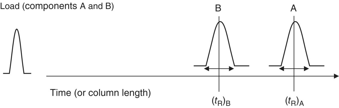
FIGURE 17.3 Schematic illustrating band broadening phenomenon.
The peak broadening, which is a result of mass transfer resistances and diffusion, may result in the overlap of the peaks of components A and B. The best separation can be achieved if there is no overlap between the peaks of components A and B by the time the whole packed bed length is traversed. Hence, the overlap caused in part by mass transfer plays a key role in achieving the desired level of purification. The characteristics of mass transfer in a packed bed under flow have been extensively studied [21]. The effect of mass transfer on separation of components and purification efficiency is described by the term resolution. Resolution is described by the following equation:
where
- (tR)A is the retention time of early eluting peak.
- (tR)B is the retention time of late eluting peak.
- WA is the width of early eluting peak.
- WB is the width of late eluting peak.
The higher the separation efficiency, the better the resolution of the column. Concepts of height equivalent to a theoretical plate (HETP) and residence time distribution have been successfully applied to quantify efficiency of a chromatography column. The van Deemter equation describes various mass transfer phenomena ongoing during chromatography, their impact on efficiency (as quantified by HETP), and the operating parameters that impact mass transfer. The resistance to mass transfer results in what is commonly referred to as “band broadening,” i.e. broadening of the peaks as they travel through the column as mentioned earlier. Higher HETP represents more “band broadening” and less separation efficiency. According to the van Deemter equation [22], the HETP is composed of three terms that describe three different mass transfer mechanisms:
where
- A represents eddy diffusion resulting from flow path inequality.
- B represents molecular diffusion.
- C represents all other resistances to mass transfer [21, 23].
- u is the interstitial velocity defined by
HETP is expressed in the unit of length. As the flow rate increases beyond an optimum, the van Deemter equation predicts that for conventional media the efficiency of the column decreases (leading to increased plate height) (Figure 17.4). In addition to the van Deemter equation, many other mathematical relationships have been derived to model the band broadening phenomenon [21].

FIGURE 17.4 Van Deemter equation is the most commonly used model for “band broadening” in chromatography. For conventional media (plot shown), the resolving power decreases as the flow rate increases.
Having an understanding of how various parameters impact the efficiency of the column is critical for large‐scale operation. A compromise in efficiency may lead to loss in yield, effective binding capacity, and product quality attributes such as purity. Acceptance criteria are generally established during process development and applied during commercial manufacturing to ensure that a chromatography column has the requisite separation efficiency (as measured by HETP) and appropriate peak shape during use. More recently, transition analysis is being used to get a more comprehensive understanding of column efficiency and packed bed integrity and will be discussed later in this chapter. The van Deemter equation suggests that bead diameter and flow rate play a key role in mass transfer. Interestingly, the selection of these two parameters is based less on any mass transfer calculation and more on practical limitation set by acceptable pressure drop across the packed bed and capability of equipment in use. In addition, for columns in excess of 1 m diameter, time and cost sometimes determine the selection of normal operating range for flow rate. Despite these economic considerations, the scale‐up principles are indeed based on the engineering fundamentals. Linear flow rate and bed height are generally held constant during scale‐up to ensure that the mass transfer conditions under which the process was developed remain consistent across scale. As mentioned previously, this allows maintaining (or at least the best effort is made) comparable yield and purity from process development to commercial manufacturing.
Concepts of chemical engineering have also aided in the development and characterization of novel types of chromatographic media as highlighted by development of perfusion media. In perfusion media (e.g. POROS® from Applied Biosystems, Foster City, CA), the pore structure is controlled such that a balance is maintained between the diffusive and convective mass transfer. This is achieved by having a certain percentage of “through pores” in the beads in addition to the network of smaller pores that branch from the “through pores.” The “through pores” do not end within the beads and thus serve as transportation highways for solutes through the beads. The “through pores” with pore diameter greater than 5 nm maintain high degree of intra‐particle mass transfer compared to diffusive (non‐perfusive) media, whereas the smaller pores branching from them (diameters in the range of 300–700 Å) provide the adequate binding capacity [23]. Thus, such media can retain efficiency at significantly higher flow rates compared with conventional diffusive media, such as agarose‐based beads. Tolerance to high flow rates and pressures enables the perfusion media to be the media of choice for high‐throughput analytical chromatography.
17.3.3.2 Flow Distribution in Chromatography Columns
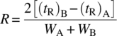
A chromatography unit operation consists of process steps such as equilibration, loading, washing, elution, and regeneration. The aim of these steps is to achieve the right condition for ligand binding, facilitate target/ligand interaction, collect the purified target protein, or restore the ligand to the initial state for the next batch. Each of these steps is carried out by flow of predetermined volumes of fluid through the column. For acceptable performance of these individual steps and the chromatography operation as a whole, uniformity of flow distribution across the column cross section is critical. Uniform flow distribution is a prerequisite for ensuring comparable mass transfer throughout a large commercial size column. Little attention is paid during bench‐scale process development to flow distribution, since for small columns, typically of 1–3 cm in diameter, this is not a major concern. The column frit is sufficient to achieve adequate flow distribution. As the diameter of the column increases, achieving a uniform flow distribution becomes increasingly difficult. The design of the column head plate plays a key role in flow distribution and the efficiency of the packed bed [24]. Computational fluid dynamics (CFD) can be successfully utilized to assist in the design of chromatography column hardware [25]. CFD utilizes fundamental fluid mechanical and mass transport relationships, representative boundary conditions, and mathematical algorithms to predict fluid properties in a variety of fluid flow scenarios. Recently, the pharmaceutical industry has shown increasing interest in CFD for providing insight into flow characteristics and related phenomena that can help mitigate risks associated with scale‐up as well as in troubleshooting [25]. Further CFD discussion can be found in Chapters 12 and 13. Frontal analysis techniques such as dye testing can be used to study the flow distribution. In brief, dye is injected into a packed and equilibrated column and allowed to flow for a predetermined period of time. Subsequently, the column is dismantled to expose the resin bed. Upon excavation, the dye profile in the bed reveals the quality of flow distribution. Alternatively, one can also look at the washout of the dye front from a column under flow and evaluate the effectiveness and uniformity of the column cleaning conditions. An appropriate cleaning procedure would be indicated when little or no residual dye is left, which can be confirmed by excavation of the resin bed after fluid flow through the column simulating the cleaning conditions.
It is ideal to use a complementary approach where CFD is used early in the hardware design process to ensure that predicted flow distribution is appropriate. Subsequent to the fabrication, dye testing can be performed to confirm the uniformity of flow distribution and flow conditions. This approach was utilized for characterization of flow dynamics in a process chromatography column [25]. A few highlights of this study are shown here. Figure 17.5 shows liquid velocity profile predicted by CFD (light gray color is low velocity and dark gray color is high velocity on the CFD tracer model picture) within a packed bed under specific flow rates with clear areas of stagnation. Subsequently, when dye testing was performed, as shown in the lower panel of Figure 17.5, the same areas failed to show dye washout demonstrating zones of stagnation and confirmed the predictions from CFD modeling.
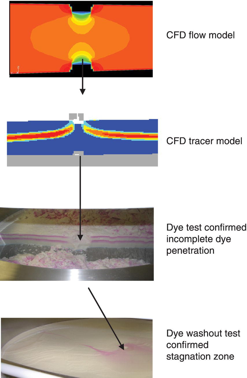
FIGURE 17.5 CFD flow and tracer modeling predicted stagnation zone beneath the chromatography resin introduction port that was confirmed by dye test.
Why is flow distribution so critical for the success of large‐scale chromatography? In addition to the issue of mass transfer and its relationship to purity and yield, there are many other factors that come into play for manufacture of biopharmaceuticals using chromatography. Without appropriate flow distribution, part of the packed bed may remain unreachable for the process fluids. This reduces the total binding capacity of the bed and underutilizes expensive chromatography media such as protein A media. The lack of flow uniformity and pockets of stagnation within the bed also increases the possibility of suboptimal cleaning and elevates the risk of microbial growth and protein carryover from one manufacturing batch to the next, creating significant safety and compliance concerns.
The chromatography system or “skid” design should ensure that appropriate flow can be delivered without excessive pressure drop from system components. Skid components (e.g. pumps) and piping should be selected appropriately to meet this requirement. The chromatography media used for biotechnology products are generally compressible and hence cannot withstand pressures in excess of three bars, thus putting practical limitation on flow rates and bed heights.
17.3.3.3 Column Packing and Packed Bed Stability
Column packing for compressible resins is generally achieved by delivering a predetermined amount of media slurry to the column followed by packing the bed to a predetermined bed height. The slurry amount and the bed height are related such that the resin bed, upon achieving the target bed height, is under a target compression. The compression factor can be recommended by the manufacturer of the chromatography media or can be determined experimentally. In either case it should be confirmed during packing development. Several engineering considerations are relevant during scale‐up and commercial manufacturing to ensure that packed bed is fit for use. As mentioned earlier, due to the compressible nature of most of the chromatography media, operations are limited to lower pressures only. In a small‐scale column with a smaller diameter, a significant part of the packed bed is supported by the frictional forces between the bed and the column wall. This is termed as the “wall effect.” As the diameter of the column increases, the extent of the “wall effect” decreases. As a result, for the same bed height and flow rate, the pressure drop increases as the column diameter increases. Work performed by Stickel and Fotopoulos [26] can be used to predict pressure drop for larger columns once the data from the small scale is available. Additional work has been performed recently in an effort to improve the prediction models [27].
Column packing is time and resource intensive. For commercial manufacturing, the columns, once packed, are used for many cycles. This mandates that the packed bed remain stable and integral during multiple uses over long periods of time. Tools have been developed to measure and monitor bed stability. Qualification tests can be performed using these tools upon completion of packing. Traditionally, this has been done by injecting a tracer solution (e.g. salt solution or acetone, usually 1–2% of the column volume) and recording the output signal (either solution conductivity or absorbance of an ultraviolet light beam) at the column exit. Peak attributes are then used to calculate HETP and asymmetry (Af) and compared to predetermined acceptance criteria. It should be noted that due to the significant resistance to protein mass transfer inside a bead, estimated plate heights for protein solutes are much greater than those obtained using a salt or an acetone solution. Hence, the results of column qualification are primarily indicative of packing consistency and integrity rather than the extent of protein separation [28]. Transition analysis, a noninvasive technique for monitoring the packed bed, is finding increasing utilization in process chromatography. Transition analysis is a quantitative evaluation of a chromatographic response at the column outlet to a step change at the column inlet [29]. It utilizes routine process data to calculate derived parameters that are indicative of the quality of the packed bed. All, or a subset of these parameters, can be used to qualify the column after packing and subsequently during the lifetime of the column to assess bed integrity.
Moreover, a robust column packing procedure needs to ensure that the amount of resin packed in the bed is accurate and reproducible. This is achieved by effective mixing of media slurry, accurate measurement of media fraction in the slurry, and the slurry volume. Application of chemical engineering concepts can help ensure success of these measurements.
17.3.4 Filtration
Filtration is used across pharmaceutical and biopharmaceutical industry spanning all phases of drug development and commercialization. It provides a “quick” option to achieve a size‐based separation. This is especially true when the difference in the molecular weight/size is significant (one order of magnitude or more). For this reason research laboratories have used filtration as a workhorse in a variety of applications ranging from buffer exchange (dialysis) to removal of particulates. Similar to discussions presented in the chromatography section, generally, yield is not a major performance parameter at the laboratory scale. Also, the filter and system sizing are not rigorously performed. It is generally based on picking an “off‐the‐shelf” item that is judged to best suit the needs. In large‐scale operation, yield is a major consideration, especially when the protein is expensive to produce. Appropriate filter sizing is also important as it determines the filtrate quality, time of operation, and cost.
At the heart of achieving separation by filtration are the membranes and filter media that provide the pore structure and size required to meet the separation performance requirement. Even though the primary mechanism of separation is based on size, in many cases, that alone is not sufficient, and charge interaction and/or adsorption is also exploited. Manufacturers of filter membranes do not always follow the same methodology to rate the membranes for pore size. Therefore, the rating provides only a first approximation of the retention capability of the membrane. Based on pore size and filter media structure, three broad categories exist as described in Figure 17.6. These categories and their application will be discussed in this chapter.
FIGURE 17.6 A comparison of filter media with respect to retention efficiency and pore size.
Filtration is performed primarily in two modes – normal flow and tangential flow (Figure 17.7). In NFF the bulk flow on the retentate side is normal to the filter surface. During the course of filtration, particulates that are not allowed to pass through the filter can either plug the pores or build a residue cake on top of the filter. Both of these events lead to reduced flux, which may then lead to selection of larger filter surface area if process time is a major consideration. The theoretical models describing filtration are based on the relationship between pore dimensions and nature of components being filtered out and use pore plugging or cake buildup, or both as primary mechanism. Gradual pore plugging occurs when small deformable particles build up on the inside of the pores (Figure 17.8). The particles restrict flow through the pores and the flow decreases. At first, the flow decays relatively little, but as the effective diameter of the pores decreases further, the pace of the blockage and the resulting flow substantially decays (Figure 17.9). The gradual pore plugging model is recognized as most applicable to biological process streams.

FIGURE 17.7 An illustration of resistance to flux during the two modes of filtration. Components that penetrate the filter result in fouling. The components that build up on the surface result in the formation of cake and concentration polarization layer. Concentration polarization can be controlled by tangential flow.

FIGURE 17.8 Mechanism and models for sizing normal flow filtration. Gradual pore plugging model is recognized as most applicable to biological processes.

FIGURE 17.9 Retention mechanism and progression of filtration.
The buildup on the surface, referred to as formation of concentration polarization or gel layer, results in increased resistance to flow, which is undesirable. The TFF mode of operation attempts to mitigate this undesirable situation by having the flow parallel or tangential to the filter surface (Figure 17.7). This tangential flow, also called cross‐flow, creates a “sweeping” action, resulting in less gel layer and increased filtrate flux. Chemical engineering principles and empirical modeling have been extensively used to model membrane fouling and gel layer formation and understand their relationship to operating parameters. This understanding leads to successful process development and scale‐up of filtration. The flux through the filter can be expressed as the ratio of driving force (i.e. transmembrane pressure) and the net resistance as shown below:

where
- J is the flux through the membrane (commonly in L/m2‐h).
- TMP is the transmembrane pressure defined as the difference of average pressures on the retentate and permeate side of the membrane.
- Rm is the resistance to flow through the membrane.
- Rg is the resistance to flow through the gel layer.
- Rf is the resistance to flow due to membrane fouling.
Empirical correlations relating flux to tangential flow rate under laminar and turbulent flow conditions have been developed [30].
Normal flow filters can be further classified as depth or membrane filters. Depth filters are used for clarification and prefiltration with higher solids content. They remove particles via size exclusion, inertial impaction, and adsorption. They have high capacity for particulate matter and lower retention predictability. Membrane filters are generally used for prefiltration and sterilization. In membrane filtration, particles are removed via size exclusion. Membrane filters have very high retention predictability. Tangential flow filters are also membrane filters but with capability to retain various molecular sizes. Microfiltration devices are made of membranes that can retain cells, cell debris, and particulate matter of comparable size. Microfiltration can be utilized for separation of cells from the cell culture fluid at harvest. Ultrafiltration is used for concentration of protein solutions or for buffer removal or exchange. Most ultrafiltration operations in large scale are performed in the tangential flow mode to maximize throughput and minimize process time.
In order to successfully use filtration in a biopharmaceutical manufacturing process, the following three steps should be followed: (i) Correct filter type and mode of operation should be selected. (ii) Filter size should be optimized for the type and quantity of product. (iii) System components (e.g. pumps, piping, housing, etc.) and size should be optimized for the application. Chemical engineering principles related to filtration play a key role in filter selection and determination of optimal size. Principles related to pumps and fluid flow through pipes must be considered to ensure that the system is sized appropriately.
17.3.4.1 Filter Selection and Sizing
At a high level, filter selection and sizing is based on three primary elements: (i) chemical compatibility, (ii) retention, and (iii) economics.
17.3.4.1.1 Chemical Compatibility
The process streams in biotechnology generally do not contain harsh chemicals, and therefore, chemical resistance to process streams is not a major concern. The filters operated in NFF mode are typically not reused and do not require cleaning. The filters operated in TFF mode are typically reused and are cleaned after every use. These membranes need to be compatible with cleaning agents such as sodium hydroxide, sodium hypochlorite, or detergent. Given that many biopharmaceuticals are injectables, the material of construction of a filter should be such that it does not add significant amounts of leachables and extractables into the product. In addition, material chosen should not result in high levels of adsorption of the product as it may lead to significant yield loss. Chemical engineers working in biopharmaceutical industry are responsible for selecting the appropriate material of construction for the filters used. Knowledge of materials sciences and polymer sciences are important in successful filter selection.
17.3.4.1.2 Retention
At the initiation of the selection and sizing process, a well‐defined design requirement is finalized. This requirement, at minimum, consists of (i) nature of the process fluid and components desired to be retained/not retained during the filtration step, (ii) volume of process fluid that will undergo filtration, and (iii) total time allowed for execution of the filtration operation. The required retention characteristic of a specified process fluid will generally steer the selection in the target range of pore size and membrane type as shown in Figure 17.6. Generally, for primary recovery steps such as separation of cells from the cell culture fluid or removal of large particulates from the process stream, depth filters are used. Filtration mechanisms in depth filters include size‐based exclusion, charged interaction, and impaction. Complete depth of the filter is utilized for catching particulates. Generally for complex mixtures, a filter train is used where different types of filters may be placed in sequence. Alternatively, newer filtration products that have multiple layers of different filtration media assembled in one unit can also be utilized. Membrane filters are typically placed at the end of depth filters to obtain particulate‐free process fluid. These can be nominally rated, or absolute rated, or a combination of the two. Absolute rated filters follow a strict cutoff that allows retention of particles above a certain size. Unlike depth filters, only the topmost layer of a membrane filter is responsible for separation. The rest of the filter serves as a mechanical support that prevents the filtering layer from collapsing under pressure from the process fluid.
Ultrafiltration is utilized to remove or exchange soluble components from a protein solution. Its widespread use in biopharmaceutical processes includes removal of smaller molecular weight process additives, removal of small organic compounds, change of buffer system to impart special properties to the protein, and concentration of a protein solution. Ultrafiltration membrane filters have the smallest pore size. Filters composed of primarily polyether sulfone or regenerated cellulose in the range of 5–300 kDa nominal molecular weight cutoff are commercially available.
17.3.4.1.3 Filtration Economics
Upon deciding the type of the filter that will be most suitable for the application, determination of appropriate size of the commercially available unit is the next step. Many choices exist in filtration with multiple suppliers providing an array of filtration products with respect to filter type, size, material of construction, pore size, mode of operation, and cost. Some filters are manufactured for specific applications such as virus filters that are used to obtain validated levels of virus reduction in the process stream. Filter selection process requires determination of required filter size for these competing products so that a primary and a backup can be selected. The aim is to achieve design requirements using minimum area, i.e. maximize flux during filtration. The filter selection and sizing is, in large part, an experimental process. However, chemical engineering principles, as they apply to filtration, have been extensively used to understand and model flow through the filters so that the experimental design is optimal. Sizing of filter is often done experimentally by determination of a filter's maximum “filterable” fluid volume before plugging (Vmax) using the actual process fluid. A characteristic curve generated by such experimentation is shown in Figure 17.10. The Vmax can be subsequently used to determine the minimum filter area required per unit volume of process fluid as shown in the following equation:

where
- Amin is the minimum filter area.
- VB is the batch volume.
- tB is the batch processing time.
- Ji is the initial filtrate flux.
The actual filter area recommended is always greater than the minimum area but generally is based on economic factors like filter cost and processing time.

FIGURE 17.10 Filter sizing experiment using gradual pore plugging model. Process solution is filtered at a constant pressure at lab scale. Volume of solution filtered (V) with respect to time (t) is recorded and plotted as shown above. Filter with the highest Vmax will result in least area requirement.
TABLE 17.3 Simulated Data from a Bench‐Scale Filtration Study
| Elapsed Time, t (min) | Volume Passed, V (ml) |
| 0 | 0 |
| 3 | 91 |
| 6 | 272 |
| 12 | 496.6 |
| 17 | 683.5 |
| 22 | 607.5 |
| 27 | 896 |
| 32 | 964 |
| 37 | 1034 |
| 42 | 1123 |
| 47 | 1195.1 |
| 52 | 1246 |
| 57 | 1295 |
| 62 | 1346 |
| 67 | 1402 |
| 69 | 1416 |
TABLE 17.4 Laboratory‐Scale Filtration Study Results for Comparison of Two Depth Filters
| Elapsed Time (min) | Depth Filter 1 | Depth Filter 2 | ||||
| Weight (g) | Throughput (L/m2) | Pressure (psig) | Weight (g) | Throughput (L/m2) | Pressure (psig) | |
| 0 | 0 | 0 | 0 | 0 | 0 | 0 |
| 5 | 20.7 | 8.28 | 0.5 | 18.1 | 7.24 | 1.4 |
| 10 | 44 | 17.6 | 1.1 | 40.1 | 16.04 | 2.5 |
| 15 | 67.5 | 22.0 | 1.5 | 62.2 | 24.88 | 3.6 |
| 20 | 90.8 | 36.32 | 1.8 | 84.6 | 33.84 | 3.8 |
| 25 | 114.2 | 45.68 | 2.2 | 106.7 | 42.68 | 4.2 |
| 30 | 137.6 | 55.04 | 2.5 | 128.8 | 51.52 | 4.5 |
| 35 | 160.7 | 64.28 | 2.7 | 151.1 | 60.44 | 5.3 |
| 40 | 183.9 | 73.56 | 3.3 | 172.8 | 69.12 | 7.3 |
| 45 | 207.1 | 82.84 | 4.7 | 194.7 | 77.88 | 9.9 |
| 50 | 230.2 | 92.08 | 7.6 | 216.7 | 86.68 | 13.4 |
| 55 | 253.2 | 101.28 | 11.9 | 238 | 95.2 | 18.4 |
| 55.5 | 255.6 | 102.24 | 13.1 | 240.2 | 96.08 | 20 |
| 60 | 276.2 | 110.48 | 18.7 | — | — | — |
| 61 | 280.8 | 112.32 | 19.9 | — | — | — |
Note: The throughput and pressure data were collected at 30 second intervals during the filtration study. For space considerations for the data table, the data are shown in five minute intervals.
FIGURE 17.11 A plot of pressure vs. filter throughput for filter selection problem in Example Problem 17.3. Once the pores start to plug from cells and cell debris, the pressure rapidly goes up. In this case, a limit of 20 psig was recommended by the filter manufacturer. Depth filter 1 provides a higher throughput without a process‐relevant increase in the turbidity.
17.3.4.2 System Sizing and Selection
Similar to the chromatography system, the filtration system design should ensure that appropriate flow can be delivered without generating excessive pressure from system components. The process control is designed such that the normal flow through the membrane (flux) and tangential flow (retentate) can be monitored and controlled by the system. Flux in NFF is generally controlled by the differential pressure across the filter. In the case of TFF, both transmembrane pressure, a measure of differential pressure across the membrane, and tangential flow are used to control the flux. The control system should ensure that maximum allowable filter pressure is not exceeded. The filters used in NFF mode are placed in housings generally of stainless steel construction. All stainless steel components are designed to be able to withstand clean‐in‐place and steam‐in‐place conditions. The housing design ensures that all entrapped air can be removed so that complete filter area comes in contact with process fluid. Many filters are self‐contained capsules that do not require housings. These types of self‐contained and single‐use filter systems are gaining popularity rapidly since they provide significant advantages by eliminating complicated setup and dismantling, shortening process time, and eliminating cleaning and sterilization.
17.4 SPECIALIZED APPLICATIONS OF CHEMICAL ENGINEERING CONCEPTS IN BIOLOGICS MANUFACTURING
In the preceding sections, we discussed how fundamental chemical engineering principles are used in process and equipment design for biologics manufacturing. In this section, we will examine how the area of process systems engineering in chemical engineering discipline offers unique solutions in biologics process development and manufacturing. Similar to a chemical plant, a biopharmaceutical plant utilizes the basic principles of mass, heat, and momentum transport to cultivate cells and produce product from raw materials and nutrients supplied to the cells and then to purify the protein in the final dosage form. Also similar to a chemical plant, a biopharmaceutical plant consumes energy and uses utilities such as water, steam, and compressed air. Because of these similarities, techniques for modeling of chemical plants can also be adapted to model a biopharmaceutical plant and the production processes.
Development of process models allows obtaining greater process understanding and predicting process behavior and is the first step toward process monitoring and control. Various levels of complexities can be incorporated in a process model. In biopharmaceutical manufacturing processes, it can vary between simple empirical models (data driven) to more sophisticated mathematical means such as metabolic flux and pathway models [31–33]. Comprehensive process understanding is imperative in achieving industry‐wide guidelines set by regulatory agencies to promote quality‐by‐design (QbD), which is building quality in the process and product design. This can be achieved via correlative, causal, or mechanistic knowledge and at the highest level via first principles models [34].
First principles modeling involves in‐depth understanding of the process dynamics that is typically defined in a set of material and energy balances via differential and algebraic equations and, depending on the modeling objectives, partial differential equations. As they demonstrate the process understanding at a highest level and provide opportunities for advanced process control, first principles models are desirable, and industry is encouraged by regulatory agencies as mentioned in various guidelines from US Food and Drug Administration [35, 36] and International Conference on Harmonization [37].
In this section, we will briefly review correlative (via multivariate modeling) and first principles‐based approaches by providing case studies to demonstrate their benefits and practical use.
17.4.1 A Case Study Using First Principles Modeling: Mass Transfer Models in Cell Culture
Mathematical modeling of cell culture in bioreactors has received significant attention and has been successfully utilized for design and characterization. Most of the models developed included unstructured and unsegregated modeling approaches to describe the process at high level. In this section we will demonstrate how first principles modeling is used to develop representation of dissolved carbon dioxide (dCO2) mass transfer in a bioreactor and practical use of the model in large‐scale setting.
Excess accumulation of dCO2 at high viable cell concentrations is known to result in adverse effects to cellular growth and specific productivity in large‐scale mammalian cell culture bioreactors. The accumulation can occur as a result of reduced surface to volume ratios and low CO2 removal rates [38–40]. It is also known that high dCO2 might be detrimental to protein structure and function (due to the alteration of glycosylation pattern of therapeutic protein). On the other hand, excess stripping of CO2 can alter bioreactor pH profile. Therefore, it is imperative to control dCO2 levels.
There are three main sources of dCO2 in cell culture: (i) CO2 produced by cells during respiration, (ii) CO2 addition to control pH at its desired level, and (iii) CO2 produced by dissociation of sodium bicarbonate added to culture for pH control. Dissolved CO2 mass balance in culture broth in relation to abovementioned sources are provided in the following equations [40]:
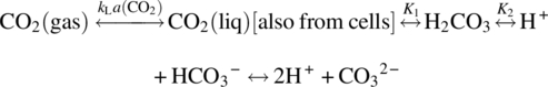
and
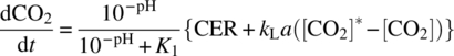
where
- kLa is mass transfer coefficient.
- K1 and K2 are equilibrium constants.
- CER is CO2 evolution rate.
- [CO2]* is the CO2 concentration at the equilibrium.
Each of these sources can be mathematically described given the cell growth and lactate generation curves as well as the bioreactor configuration and operating conditions as depicted in Figure 17.12. While more detailed generic mathematical description of the model can be found in the literature [38–40], we will focus on the industrial use of the model in this section.
FIGURE 17.12 Schematic diagram representing the main input and output structure of CO2 transport model.
The key inputs for model are the VCD and lactate concentration sampled over the time course of the bioreactor operation. In Figure 17.12, td designates discrete measurements performed, e.g. daily measurements, and t designate continuous outputs. The model receives a number of other values such as gas flow rates and base addition just for comparison purposes against model predictions for those. In other words, the model predicts those within its differential and algebraic equation set for every time instance that it solves and compares its outputs against the daily observations from the plant results. Model also allows studying the effect of pH control loop influence on the oxygen composition of the sparge gas so that controlling the levels of dCO2 can be improved. Once a model is developed, it should be tested with existing process data, and the output should be compared against the process outcome. In this case, the model was tested against large‐scale production bioreactor data and found to be predictive of known performance. The model was able to provide a predicted relationship between CO2 flow rate and dissolved CO2 when the cell growth (VCD) and lactate concentration ([Lac]) time courses are provided and pH and aeration are at control set points. The predictive model can be utilized in a variety of applications. Perhaps the most beneficial application of such a model is in its ability to predict process behavior in a scale‐up. During process development, a large body of small‐scale process data is generated. These data can be used in the development of the model. Typically, the process is then scaled up to a pilot scale with perhaps a handful of process runs at that scale. Further refinement of the model can be performed with this data, and scale comparability can also be assessed. The model can then be utilized to make predictions of large‐scale process conditions.
In our specific scenario, the model was being utilized to evaluate process behavior of a follow‐on (second‐generation) process when a current process was already being operated at large scale. Therefore, we had access to process data at small, pilot, and large scales for the current (legacy) process. The follow‐on process had small‐scale and some pilot‐scale process data. The scenario can be pictorially represented in Figure 17.13. The follow‐on process was expected to have much higher cell densities, and we were interested to know how we would select certain design criteria for large‐scale bioreactors. One such criterion was the size of the mass flow controller that determines the amount of gas input to the culture. As can be seen from Figure 17.13, there were no process data available from a large‐scale bioreactor (since no follow‐on process had been run at this scale, yet, at that time). The approach undertaken was to first utilize the CO2 first principles model for the current process to ensure that the predictions are comparable to what was observed at both pilot and the large scales from historical runs. Once that was confirmed, the follow‐on process conditions were used to generate predicted values at pilot scale. Since we had pilot‐scale data from the follow‐on process, we could verify that the model was still predictive. The final step was then to run the model using the large‐scale bioreactor conditions with expected follow‐on process metabolic response (VCD and lactate concentrations) to predict the dCO2 levels that might be seen at large scale. This then allowed us to do appropriate calculations and size selection of large‐scale sparge equipment.
FIGURE 17.13 Color map representation of the available runs and data across scales (darker color means more manufacturing runs are available).
In another application of the first principles CO2 model, we evaluated the impact of reducing agitator tip speed in our process. As mentioned earlier, the agitator speed is linked to mass transport in the culture but also can be a concern for shear or for the effect of air interface on the cells. Using our model we were able to predict the culture properties at a lower agitator tip speed and determine whether our existing systems would be adequate for supporting the process requirement. Figure 17.14 shows some of the output of the model and demonstrates that for the most part key parameters such as pCO2, pO2, pH, etc. are comparable at different tip speeds. Despite the reduced agitation speed and aeration, DO was maintained at the required set point (mass transfer from gas to liquid is not rate limiting with respect to its consumption). Increase in sparged O2 has allowed to attain the DO set point. Predicted increase in the demand on the sparged CO2 under these conditions was well within the delivery capability of the existing mass flow controllers, and therefore, no resizing was required.

FIGURE 17.14 Simulation results for agitator tip speed reduction, effect on CO2 and O2 requirements. Solid line (─), high agitation speed and high aeration rate; dashed line (‐ ‐), reduced agitation speed and aeration rate.
In these examples, use of a first principles model has shown its benefits by providing guidance for scale‐up decisions without having to run actual experiments at scale, which is a costly activity. It has also helped increase process understanding of scale‐up between pilot and large scales and provided performance comparability. Having a reliable first principles model provides bioprocess engineers ample opportunities for process optimization, troubleshooting, and improvement and supports engineering decision‐making process.
17.4.2 Application of Statistical Models in Process Monitoring and Control of Biologics Manufacturing Processes
There are challenges in modeling, monitoring, and control of batch biopharmaceutical processes due to their inherently complex biological and biochemical mechanisms and nonlinear time‐variant process dynamics. There are also many variables measured during the course of a batch either offline or online and at variable frequencies depending on the measurement system used. It is important to efficiently monitor and diagnose deviations from the in‐control space for troubleshooting and process improvement purposes. One of the solutions successfully applied in chemical industry (both batch and continuous processing) is multivariate modeling and real‐time statistical process monitoring [41–43]. These applications have been also successfully extended to pharmaceutical and biopharmaceutical cases [44–47].
In a typical industrial setting, data is generated by the process via various equipment online controls, offline measurements, and assays, which are all stored in various databases. Many process batches (I) are executed, where many variables (J) are measured at certain time intervals (K), forming a three‐way data array (X) as depicted in Figure 17.15. Developing data‐driven multivariate process models that define process variability has been shown beneficial in proactively monitoring the process consistency and performance and in troubleshooting purposes. Typical process performance (as contained within data array X from the process variables shown in Figure 17.15) can be modeled using multivariate techniques such as principal component analysis (PCA) and partial least squares (PLS). PCA is used when overall variability is to be modeled to find major variability dimension in a process (as shown for three variables in Figure 17.16a). This way the dimensionality problem is solved by reducing from many raw process variables to a few derived variables called principal components (PCs) that have linear contributions from raw variables. If the objective is also to correlate how changes in process variables impacting, say, a performance variable defining an endpoint, then PLS is the preferred choice. In that case, the multivariate regression model (PLS) is fitted to data from process variables (inputs) in such a way that it maximizes the correlation to response variable (process output or endpoint). These techniques are extremely useful including (i) reducing the dimensionality problem (summarizing the overall process variability into a few variables from many), (ii) explaining the correlation structure of the variables, (iii) handling missing data, (iv) reducing the noise inherent to measurements so the actual signal can be extracted, and (v) providing means for multivariate statistical process monitoring (MSPM) of the entire process (Figure 17.16).
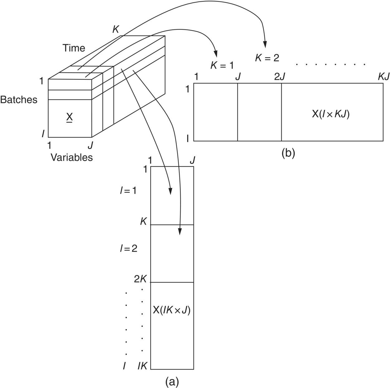
FIGURE 17.15 Unfolding of three‐way batch data array: (a) observation level, which preserves variable direction, and (b) batch level, which preserves batch direction.
FIGURE 17.16 (a) Dimensionality reduction of a three‐variable (x1, x2, and x3) process. Overall variability of the process can be explained by using two principal components (Cinar et al. [33]). (b) Multivariate SPC vs. univariate SPC (MacGregor and Kourti [41]), a batch observation (depicted with a circled‐cross sign) that is in control in univariate charts is actually out of control in bivariate in control region defined by the ellipsis (95% confidence region).
MSPM for batch (bio) processes can be achieved in real time. Setting the framework up involves the following steps:
- Collect historical batch data (from typically 20–30 batches of many process variables that are measured online) that define normal operating region.
- Detect and remove outliers in the data and apply preconditioning (autoscaling).
- If the objective is only fault detection and diagnosis, develop a PCA model, and if the objective is also to predict process performance variables or critical quality attributes in real time, develop multivariate regression models such as PLS.
- Construct multivariate charts for real‐time monitoring. Monitor a new batch by projecting its data (applying the same data conditioning) onto the model spaces that are developed for comparing to nominal performance.
PCA and PLS are performed on the unfolded array (X) in either direction as shown in Figure 17.15. Observation level models are suggested to avoid estimating the future portion of new batch trajectories [48]. These models are used in real‐time monitoring of a new batch, whereas batch‐level models are used at the end of the batch for analyzing across batch trends, also known as “batch fingerprinting.” Details and mathematical formulation of the modeling in PCA and PLS for batch processes (when it is performed for batch processes, they are usually referred to as multiway PCA or PLS models) can be found in the literature [46, 48].
A number of multivariate statistics and charts are used for monitoring new batches in real time. These include:
- Squared prediction error (SPE) (also known as Q‐residuals or DModX) chart
SPE is used for process deviation detection where events are not necessarily explained by the model. When SPE control limit violation is observed, it is likely that a new event is observed that is not captured by the reference model (this can be triggered by a normal event that is part of inherent process variability that is not captured or a process upset).
- Score time series and Hotelling's T2 charts
These charts are also used for process deviation detection. They allow detecting deviations that are explained by the process model and within the overall variability but represent unusually high variation compared to the average process behavior. Score time series allow monitoring the process performance at each model dimension separately, while T2 allows monitoring all of the model dimensions over the course of a batch run by using a single statistic calculated from all scores.
- Contribution plots
When the detection charts above identify a deviation (violation of multivariate statistical limits on SPE and/or T2 charts), which indicates that some variables or variable is deviating from the historical average behavior without diagnosing which variables are contributing the most. Contribution plots are then used to delve into the original variable level to inspect which variable or variables are contribution to the inflated statistic.
17.4.2.1 Utilization of Real‐Time Multivariate Statistical Process Monitoring in Bioprocessing
MSPM tools provide an important means to rapidly detect process anomalies as the process is running and take action to correct issues before the process drifts to an out‐of‐control region. In our example, an MPCA model was developed (steps are described above) for a train (multiple systems operated in an alternating fashion across batches) of a perfusion bioreactor system (bioreactor, TFF skid, and the media tank). The model used historical process data measured on 21 variables from a statistically relevant number of batches throughout the operation that typically spans several days, yielding thousands of data points. Ninety‐six percent of overall process variability could be explained by only using three PCs in this multivariate model.
When a transient decline (~3%) was observed in final day viability (measured by an offline analytical system) in the bioreactor across batches (Figure 17.17a), deviations were also seen in real‐time multivariate charts (Figure 17.17b; Hotelling's T2 chart for one of the low viability batches is shown). Variable contribution plots (Figure 17.16c) identified that higher perfusion feed and retentate temperature conditions occurred in the equipment in comparison to the normal process behavior demonstrated by the historical batches. Further investigation revealed that an equipment mismatch in the system caused the higher than normal temperature. The issue was corrected prior to the next batch, and the temperature profile and final day viability returned to their normal ranges (lower left corner of Figure 17.16b).

FIGURE 17.17 Real‐time multivariate statistical process monitoring (RT‐MSPM) steps involved in troubleshooting of a perfusion bioreactor system (shown in c): (a) offline observation of viability decline, (b) detection via T2 charts, (c) contribution plot for diagnosing the potential root cause, and (d) inspection of the univariate variable profiles.
The example provided here demonstrates how MSPM can detect an abnormal process behavior, assist in determination of root cause, and confirm when a resolution is implemented and the process has returned to normal. The technology has the potential to increase operational success and reduce production costs in highly complex biopharmaceutical processing systems [49].
17.5 CONCLUSIONS
Since the time of synthesizing penicillin in milk bottles in the 1940s, bioprocesses have come a long way. Today, bioprocesses are used for commercial manufacturing of biologics that include therapeutic proteins, vaccines, enzymes, diagnostic reagents, and nonprotein complex macromolecules such as polysaccharides. Biologics are expected to be a major sector within the life sciences industry. The global market for biologics, currently at about $48 billion, is expected to rapidly grow to about $100 billion in the next few years. Currently 6 out of 10 best‐selling drugs are biotechnology derived, and over a third of all pipeline products in active development are biologics. The pipeline amounts to approximately 12 000 drug candidates in various stages of preclinical and clinical development covering about 150 disease states and promises to bring better lifesaving treatment to patients. These staggering statistics demonstrate that the fundamentals of biologics and bioprocess industry are strong.
Industrial biotechnology requires blending three key disciplines – biology, biochemistry, and chemical engineering. While our focus in this chapter has been on application of chemical engineering principles to biotechnology, we urge the readers to recognize that the principles of biology and biochemistry play equally (or more) important role in biologics and bioprocessing. Innovation is directly linked to the success of biotechnology products and processes. Innovation in protein design, genetic engineering, expression systems, and manufacturing technologies has allowed rapid commercialization of highly profitable biopharmaceutical products despite the presence of strict regulatory requirements. The innovation, however, has come at a considerable cost. Biologics are the most expensive among all medicinal products. As the biopharmaceutical industry proceeds through its evolution to maturity, it will be forced to undergo significant reinvention to include sound economic principles in addition to sound scientific and engineering principles that provide most cost‐effective and value‐appropriate therapies to patients.
REFERENCES
- 1. Stryer, L. (1988). Protein structure and function. In: Biochemistry, 3e, 15–42. New York: W. H. Freeman & Co.
- 2. Medved, L.V., Orthner, C.L., Lubon, H. et al. (1995). Thermal stability and domain‐domain interactions in natural and recombinant Protein C. J. Biol. Chem. 270: 13652–13659.
- 3. Narhi, L., Philo, J., Sun, B. et al. (1999). Reversibility of heat‐induced denaturation of the recombinant human megakaryocyte growth and development factor. Pharm. Res. 16: 799–807.
- 4. Franks, F. (1988). Conformational stability – denaturation and renaturation. In: Characterization of Proteins, 1e (ed. F. Franks), 104–107. New York: Humana Press.
- 5. Tang, X. and Pikal, M. (2005). The effect of stabilizers and denaturants on the cold denaturation temperatures of proteins and implications for freeze‐drying. Pharm. Res. 22: 1167–1175.
- 6. Maa, Y.‐F. and Hsu, C.C. (1997). Protein denaturation by combined effect of shear and air‐liquid interface. Biotechnol. Bioeng. 54: 503–512.
- 7. Thomas, C.R. (1990). Problems of shear in biotechnology. In: Chemical Engineering Problems in Biotechnology, 1e (ed. M.A. Winkler), 23–93. New York: Elsevier.
- 8. Junker, B.H. (2004). Scale‐up methodologies for E. coli and yeast fermentation processes. J. Biosci. Bioeng. 97: 347–364.
- 9. Xing, Z., Kenty, B., Jian, Z., and Lee, S.S. (2009). Scale‐up analysis for a CHO cell culture process in large‐scale bioreactors. Biotechnol. Bioeng. 103: 733–746.
- 10. Yang, J., Lu, C., Stasny, B. et al. (2007). Fed‐batch bioreactor process scale‐up from 3‐L to 2500‐L scale for monoclonal antibody production from cell culture. Biotechnol. Bioeng. 98: 141–154.
- 11. Ju, L.‐K. and Chase, G.G. (1992). Improved scale‐up strategies of bioreactors. Bioprocess Eng. 8: 49–53.
- 12. Dosmar, M., Meyeroltmanns, F., and Gohs, M. (2005). Factors influencing ultrafiltration scale‐up. Bioprocess Int. 3: 40–50.
- 13. Van Reiss, R., Goodrich, E.M., Yson, C.L. et al. (1997). Linear scale ultrafiltration. Biotechnol. Bioeng. 55: 737–746.
- 14. Prokop, A. (1991). Implications of cell biology in animal cell biotechnology. In: Animal Cell Bioreactors (ed. C.S. Ho and D.I.C. Wang), 21–58. Boston, MA: Butterworth‐Heinemann.
- 15. Nienow, A.W. (2006). Reactor engineering in large scale animal cell culture. Cytotechnology 50: 9–33.
- 16. Blanch, H.W. and Clark, D.S. (1997). Biochemical Engineering, 415–426. New York: Marcel Dekker Inc.
- 17. Xie, L. and Wang, D.I.C. (1994). Stoichiometric analysis of animal cell growth and its application in medium design. Biotechnol. Bioeng. 43: 1164–1174.
- 18. Cooper, C.K., Fernstrom, G.A., and Miller, S.A. (1944). Performance of agitated gas‐liquid contactors. Ind. Eng. Chem. 36: 504–509.
- 19. Shukla, A.A. and Kandula, J.R. (2009). Harvest and recovery of monoclonal antibodies: cell removal and clarification. In: Process Scale Purification of Antibodies (ed. U. Gottschalk), 53–78. Hoboken, NJ: Wiley.
- 20. Blanch, H.W. and Clark, D.S. (1997). Biochemical Engineering, 461–467. New York: Marcel Dekker Inc.
- 21. Usher, K.M., Simmons, C.R., and Dorsey, J.G. (2008). Modeling chromatographic dispersion: a comparison of popular equations. J. Chromatogr. 1200: 122–128.
- 22. Van Deemter, J.J., Zuiderweg, F.J., and Klinkenberg, A. (1956). Longitudinal diffusion and resistance to mass transfer as causes of nonideality in chromatography. Chem. Eng. Sci. 5: 271–289.
- 23. McCoy, M., Kalghatgi, K., Regnier, F.E., and Afeyan, N. (1996). Perfusion chromatography – characterization of column packings for chromatography of proteins. J. Chromatogr. 743: 221–229.
- 24. Moscariello, J., Purdom, G., Coffman, J. et al. (2001). Characterizing the performance of industrial‐scale columns. J. Chromatogr. 908: 131–141.
- 25. Pathak, N., Norman, C., Kundu, S. et al. (2008). Modeling flow distribution in large‐scale chromatographic columns with computational fluid dynamics. Bioprocess Int. 6: 72–81.
- 26. Stickel, J.J. and Fotopoulos, A. (2001). Pressure‐flow relationships for packed beds of compressible chromatography media at laboratory and production scale. Biotechnol. Prog. 17: 744–751.
- 27. McCue, J.T., Cecchini, D., Chu, C. et al. (2007). Application of a two‐dimensional model for predicting the pressure‐flow and compression properties during column packing scale‐up. J. Chromatogr. 1145: 89–101.
- 28. Teeters, M.A. and Quinones‐Garcia, I. (2005). Evaluating and monitoring the packing behavior of process‐scale chromatography columns. J. Chromatogr. 1069: 53–64.
- 29. Larson, T.M., Davis, J., Lam, H., and Cacia, J. (2003). Use of process data to assess chromatographic performance in production‐scale purification columns. Biotechnol. Prog. 19 (2): 485–492.
- 30. Lyderson, B.K., D'elia, N.A., and Nelson, K.L. (1994). Bioprocess Engineering Systems, Equipment and Facilities. New York: Wiley.
- 31. Bailey, J.E. (1998). Mathematical modeling and analysis in biochemical engineering: past accomplishments and future opportunities. Biotechnol. Prog. 14: 8–20.
- 32. Stephanopoulos, G., Aristidou, A.A., and Nielsen, J. (1998). Chapter 8: Metabolic flux analysis; Chapter 9: Method for experimental determination of metabolic fluxes by radioisotope labeling; Chapter 10: Applications of metabolic flux analysis. In: Metabolic Engineering: Principles and Methodologies, 309–459. London, UK: Academic Press.
- 33. Cinar, A., Parulekar, S.J., Undey, C., and Birol, G. (eds.) (2003). Batch Fermentation: Modeling, Monitoring and Control, 21–58. New York: CRC Press.
- 34. Rathore, A.S. and Winkle, H. (2009). Quality by design for biopharmaceuticals. Nat. Biotechnol. 27: 26–34.
- 35. US Food and Drug Administration (2002). Pharmaceutical cGMPs for the 21st Century: A Risk‐based Approach (August 2002). Rockville, MD: FDA. https://www.fda.gov/downloads/drugs/guidances/ucm070305.pdf (accessed 23 July 2009).
- 36. US Food and Drug Administration (2004). Guidance for Industry: PAT – A Framework for Innovative Pharmaceutical Development, Manufacturing, and Quality Assurance. Rockville, MD: FDA. http://www.fda.gov/Cder/guidance/6419fnl.pdf (accessed 23 July 2009).
- 37. International Conference on Harmonisation (ICH) (2008). Pharmaceutical Development Q8(R1). Geneva: ICH. https://www.ich.org/fileadmin/Public_Web_Site/ICH_Products/Guidelines/Quality/Q8_R1/Step4/Q8_R2_Guideline.pdf (accessed 23 July 2009).
- 38. Gray, D.R., Chen, S., Howarth, W. et al. (1996). CO2 in large‐scale and high‐density CHO cell perfusion culture. Cytotechnology 22: 65–78.
- 39. Zupke, C. and Green, J. (1998). Modeling of CO2 concentration in small and large scale bioreactors. Presented at Cell Culture Engineering VI, San Diego, CA (1998).
- 40. Mostafa, S. and Gu, X. (2003). Strategies for improved dCO2 removal in large‐scale fed‐batch cultures. Biotechnol. Prog. 19: 45–51.
- 41. MacGregor, J.F. and Kourti, T. (1995). Statistical process control of multivariate processes. Control Eng. Pract. 3: 403–414.
- 42. Neogi, D. and Schlags, C.E. (1998). Multivariate statistical analysis of an emulsion batch process. Ind. Eng. Chem. Res. 37: 3971–3979.
- 43. Undey, C., Ertunc, S., Tatara, E. et al. (2004). Batch process monitoring and its applications in polymerization systems. Macromol. Symp. 206: 121–134.
- 44. Westerhuis, J.A., Coenegracht, P.M.J., and Lerk, C.F. (1997). Multivariate modeling of the tablet manufacturing process with wet granulation for tablet optimization and in‐process control. Int. J. Pharm. 156: 109–117.
- 45. Albert, S. and Kinley, R.D. (2001). Multivariate statistical monitoring of batch processes: an industrial case study in fed‐batch fermentation supervision. Trends Biotechnol. 19: 53–62.
- 46. Undey, C., Ertunc, S., and Cinar, A. (2003). Online batch/fed‐batch process performance monitoring, quality prediction and variable contributions analysis for diagnosis. Ind. Eng. Chem. Res. 42: 4645–4658.
- 47. Undey, C., Tatara, E., and Cinar, A. (2004). Intelligent real‐time performance monitoring and quality prediction for batch/fed‐batch cultivations. J. Biotechnol. 108: 61–77.
- 48. Wold, S., Kettaneh, N., Fridén, H., and Holmberg, A. (1998). Modelling and diagnostics of batch processes and analogous kinetic experiments. Chemom. Intel. Lab. Syst. 44: 331–340.
- 49. Undey, C., Ertunc, S., Mistretta, T., and Pathak, M. (2009). Applied advanced process analytics in biopharmaceutical manufacturing: challenges and prospects in real‐time monitoring and control. IFAC ADCHEM Proceedings, Istanbul, Turkey (13–15 July 2009).