
4
CALORIMETRIC APPROACHES TO CHARACTERIZING UNDESIRED REACTIONS
Megan Roth and Tom Vickery
Chemical Engineering R&D, Merck & Co., Inc., Rahway, NJ, USA
4.1 INTRODUCTION
Identification and characterization of the thermal and pressure consequences of both desired and undesired reactions are critical components of assessing the safety of a process. Although the desired reactions are typically studied in depth, undesired reactions are frequently neither identified nor characterized. An undesired reaction is the reaction that occurs when as few as one process deviation such as a single human or equipment error occurs, causing the process to not run as intended. It is important to identify these hazards and understand the associated consequences in order to take the appropriate corrective actions to either mitigate or avoid the risks. This data may influence the design of the process or equipment as it feeds into associated hazard assessments (e.g. process hazard analysis (PHA), hazard and operability study (HAZOP), failure mode and effects analysis (FMEA)) [1]. The end goal is to protect people, protect equipment/facilities, and prevent disruption to the supply of medicines.
Even though it is uncommon to reach an undesired reaction that has severe consequences associated with it, when these reactions are present in a process, it is important that inherent protection is provided. A process may run for years without an incident before one day an error leads to a runaway reaction and vessel explosion. Below are excerpts from a relevant incident investigation by the Chemical Safety Board (CSB) [2] that highlights the importance of characterizing undesired reactions:
In April 1998, “an explosion and fire occurred during the production of Automate Yellow 96 Dye at the Morton International, Inc. (now Rohm & Haas) Plant in Paterson, New Jersey. The explosion and fire were the consequence of a runaway reaction, which over‐pressured a 2000‐gallon capacity chemical reactor vessel (or kettle) and released flammable material that ignited.” “Nine employees were injured, including two seriously, and potentially hazardous materials were released into the community.” “The reaction accelerated beyond the heat‐removal capability of the kettle. The resulting high temperature led to a secondary runaway decomposition reaction causing an explosion, which blew the hatch off the kettle and allowed the release of the kettle contents.”
Morton's initial research and development for the Yellow 96 process identified the existence of both a desired and undesired exothermic reaction. “The Paterson facility was not aware of the decomposition reaction. The Process Safety Information (PSI) package, which was used at the Paterson plant to design the Yellow 96 production process in 1990 and which served as the basis for a Process Hazard Analysis (PHA) conducted in 1995, noted the desired exothermic reaction, but did not include information on the decomposition reaction.” Also, there was a discrepancy in the MSDS for Yellow 96, where the boiling point was listed at 100C when the actual boiling point is approximately 330C, greater than the decomposition temperature. In addition, no action had been taken on a recommendation from 1989 to perform additional studies to characterize the reaction rate under worst‐case conditions and obtain pressure rise data to size emergency venting equipment. These findings are among various other key findings by the CSB.
Several other relevant incident investigations can also be found on the CSB website (www.csb.gov).
This chapter will build upon the introduction to process safety (Chapter 3) to provide further details about the use of calorimetric approaches for studying the undesired decomposition reaction. The approaches include the use of thermal and pressure screening tools in addition to the use of more advanced instrumentation and techniques. Instruments highlighted include differential scanning calorimetry (DSC), multiple module calorimeter (MMC), accelerating rate calorimeter (ARC), and advanced reactive systems screening tool (ARSST). Several case studies will then be presented to demonstrate the use of these tools and highlight the importance of identifying and characterizing undesired reactions.
4.2 BACKGROUND
In order to accurately assess the safety of a process, it is important to understand the consequences of heat and pressure and the importance of scale on the process risks. The selection of samples for evaluation can also have a serious impact on the effectiveness of the hazards evaluation.
4.2.1 Heat and Pressure Effects
The generation of heat by desired reaction or decomposition requires one of two things to occur: either the heat must be removed via cooling or phase change, or the batch temperature must increase. For example, a 2 J/g energy release could raise the temperature of an organic material approximately 1 K, depending on the heat capacity (typically ~2 J/g·K for an organic liquid):
Acid–base reactions typically have energies on the order of 40–60 kJ/mol. Therefore to produce a 1 K temperature increase would require only a modest reaction concentration of approximately 0.04 mol/l:

The amount of heat generated by either the desired chemistry or decomposition, and the associated temperature rise, should be used in combination with operating parameters such as batch temperature, maximum desirable temperature, vessel cooling capability, and maximum jacket temperature to determine the risk. For example, if an exothermic reaction is being heated to temperature by an electrical heating mantle, the mantle can serve as insulation, preventing the removal of heat as the temperature rises as a result of the reaction.
As the temperature increases, the rates of most reactions increase, with a general approximation that the rate doubles for every 10 K temperature increase; the exact rate of increase in temperature will depend on the activation energy. Therefore failing to remove the heat of the reaction or decomposition can lead to a rapid increase in the rate that heat is generated, which can further increase the batch temperature. This phenomenon is known as a runaway reaction and is implicated in many serious chemical incidents, such as the one in the introduction.
The total pressure present in a closed reactor has three contributors: the initial permanent gas in the vessel, which undergoes thermal expansion as a result of heating, the vapor pressure of any solvents, and the generation of additional permanent gas. The first two terms are a function primarily of the vessel temperature and are reversible. In the absence of permanent gas generation, the heat‐up and cooldown curves should be nearly identical on a plot of pressure versus temperature. First the pressure increases as the temperature increases, and the pressure decreases as temperature is cooled back to the starting temperature. One exception is when the solvent is involved in the reaction, which may shift the curve up or down. See Figure 4.1.

FIGURE 4.1 Pressure–temperature curve of a reaction mixture without permanent gas generation.
If the reaction generates a permanent gas1 such as CO2, N2, or HCl, the pressure change becomes a function of both temperature and time and is irreversible. When the heat‐up and cooldown pressure–temperature curves are plotted, the pressure during cooldown is much higher than when it was heated. The difference in pressure following heat‐up and cooldown is from the permanent gas that was generated. See Figure 4.2.
FIGURE 4.2 Pressure–temperature curve of a reaction mixture with permanent gas generation.

FIGURE 4.3 Jacket temperature vs. reactor size for the reaction modeled in Example Problem 4.2.
The total pressure generated, in addition to the rate of pressure generation, should be compared with operating parameters such as the vessel maximum allowable working pressure (MAWP) and available venting capacity to determine the associated level of risk.
By comparing two versions of a reaction, one of which generates gas, and one of which does not:
- A(l) + B(l) → C(l) + D(l)
- A(l) + B(l) → C(l) + N2(g)
we can show that even in fairly dilute conditions, the formation of gas leads to a major increase in the potential maximum pressure with associated risk increase.
4.2.2 Onset Temperature Versus Exotherm Initiation Temperature (EIT)
Throughout this chapter two key temperatures will be discussed. One is the onset temperature, which is used in discussing DSC results. This concept is discussed in Section 3.5.2; typically about a 10 mW/g heat generation rate can be detected. The other temperature is the exotherm initiation temperature (EIT), which is defined as a temperature rise rate of 0.02 K/min at a phi factor of 1.0, typically measured in an adiabatic calorimeter such as an ARC or vent sizing package (VSP), and corresponds to a heat generation rate of 0.7 mW/g for a typical organic sample [4], compared with the typical 10 mW/g threshold for DSC onset. The EIT, which is normally considered to be the temperature at which the reaction becomes hazardous, can be from 25 to 50 K or more lower than the onset temperature.
4.2.3 Scale Dependence
The scale at which a reaction is run can have a dramatic effect on the safety of process. This is commonly referred to as the “square‐cube effect” or “surface‐area‐to‐volume ratio,” where the hazard (heat generation, gas generation) increases as the cube of the “radius” (proportional to volume), while the protection available (jacket cooling, gas removal) increases as the square of the “radius” (proportional to surface area).
For example, a reaction that generates 50 W/l (~0.05 W/g) of heat might require a jacket temperature of 22 °C to maintain the 30 °C temperature at a 1 L scale, but 2 °C at a 50 L prep lab scale, and −45 °C at a 1000 L manufacturing scale (See Figure 4.3).
As the scale increases, two additional factors should be considered. One is the increased consequences of a failure; the larger the vessel, the more energy will be released if it fails. The second point is more subtle, but, as the scale increases, the process may also be becoming more routine and automated. For example, an initial pilot plant batch may have a chemist, an engineer, and several operators watching it, while in a manufacturing site a single operator may be overseeing several simultaneous batches. Therefore it is more important to understand the sensitivity of the process to deviations, and the consequences of the deviations, which may trigger increased and more sensitive testing, using adiabatic calorimetry, for example.
4.2.4 Sample Selection
In order to evaluate a process, typically it is necessary to test more than one sample (among the starting materials/reagents, process streams, and/or product). Identifying what samples should be screened for decompositions requires a consideration of several factors. Is the material or a reagent known to be unstable at reachable temperatures? Has the system undergone a chemical transformation? Has the environment changed (acidic vs. basic)? Is there a reactive solvent like dimethylformamide (DMF) or dimethyl sulfoxide (DMSO) present? Has a catalyst been added?
The goal for evaluating the desired process should be to ensure that any dangerous decompositions will be detected. Screening every stream in the process is theoretically the best way to do this, but that can lead to a large amount of low value testing, distracting from the critical samples that should be carefully evaluated. Therefore testing of select streams may be sufficient to evaluate the process, if the streams that present the highest likelihood of being process safety risks can be systematically identified.
For example, a nitro compound is dissolved in ethanol and reduced with a catalyst and hydrogen to an amine and then isolated as an HCl salt. Possible samples might include the nitro compound itself (known instability from the literature), the solution plus catalyst before hydrogen is added (does the catalyst increase instability), the solution after the hydrogenation (is the amine stable, and are unstable impurities such as hydroxylamines and nitroso compounds present), the mother liquors (contain all process impurities and may be held for an extended period of time), and the isolated amine salt, which is a new species with a new environment (acid vs. base).
Beyond the streams from the desired process, if a particular deviation from a single point of failure is considered to either be likely, or of serious consequences, then it may be desirable to assess the stream or streams that would result from the deviation. For example, a hazardous reagent such as hydrogen peroxide might be overcharged, or 5 equiv. of sodium azide instead of 1 may be used, or the hydrogenation discussed earlier might stall at 50% completion, leaving a dangerous combination of intermediates in the batch. Once the appropriate samples to test have been identified, thermal screening for heat and gas generation should be carried out.
4.2.5 Techniques for Evaluating the Thermal Behavior of Decompositions
DSC is the most common but not the only tool for evaluating the thermal behavior of decomposition reactions. Table 4.1 compares several techniques used to study them. The DSC's main advantages are small sample size and short run times. The main disadvantage is that an exotherm rate must exceed a certain threshold before it is detected, which typically means that the reported onset temperature is higher than the actual EIT, so if only DSC data is available, a conservative safety margin may need to be applied. This is the origin of the traditional “100‐degree rule” referred to in Section 3.5.2, where the exothermic activity is considered to be avoided 100 °C below the exotherm onset. As noted, in some cases this rule may not be adequate, in particular if autocatalytic activity or low activation energies are involved. A more detailed discussion of onset temperature issues can be found in Hofelich [5].
TABLE 4.1 Comparison of Calorimetric Techniques for Studying Decompositions
| Instrument | Sample Size (g) | Typical Run Time (h) | Lowest Detectable Heat Flow (mW) | Sensitivity (W/kg) | Maximum Temperature (°C) | Maximum Pressure (psi) |
| DSC | 0.005 | 0.5–5 | 0.02 | 4 | 450 | 400 |
| Small‐scale reaction calorimeter | 5 | 5–24 | 1 | 0.2 | 150 | 500 |
| Large‐scale reaction calorimeter | 100 | 1–24 | 50 | 0.5 | 200 | 150 |
| Adiabatic calorimeter | 2 | 4–72 | 2 | 0.7 | 500 | 1500 |
As the most common method for detecting the presence of decomposition exotherms, DSC will be discussed below.
4.3 THERMAL STABILITY SCREENING: DIFFERENTIAL SCANNING CALORIMETRY (DSC)
The basics of DSC screening for hazards evaluation are covered in Section 3.5.2. This section discusses some additional points to consider in using DSC testing for evaluating decompositions.
4.3.1 Cell Selection
There are several types of DSC cells and seals in common use. They differ mainly in weight, material of construction (MOC), sealing, and pressure rating.3 The cell weight affects the sensitivity and the quality of the baseline: lighter cells generally produce better signal‐to‐noise ratios. The MOC of the cell is important if a decomposition is being studied. In some cases certain materials can catalyze the decomposition (hydrazine in Hastelloy, for example). In other cases either the stream contains a corrosive material (HCl, for example) or generates a corrosive material. Corrosion reactions are highly exothermic (1/3 Al(s) + HCl(aq) → 1/3 Al+3 + 3Cl− + 3/2 H2 ΔH = −177 kJ/mol4) and can appear as false positives.
Sealing and pressure rating of the cells are related; if a DSC cell is not hermetically sealed, the evaporation of either the solution solvent or the solvate solvent (commonly water) will occur. For studying decompositions, this is undesirable for several reasons: (i) the heat loss from evaporation can mask exotherms that may occur near the boiling point. (ii) The sample no longer reflects what will be in the process equipment – it will either desolvate or turn into a neat solid or liquid, both of which can have very different onset temperatures or energies than the original sample. If the seal fails during a decomposition, all of the volatile material and any confined gases will escape, both providing evaporative cooling and decompressive cooling, thus preventing accurate evaluation of the exotherm size.
For studying decompositions up to high temperatures (~400 °C), stainless steel, Hastelloy, and gold‐ and tantalum‐lined cells with gold or gold‐plated or PTFE high pressure seals are commonly used, combining corrosion resistance, a high pressure rating, and good sealing in one package.5
Decompositions cannot normally be studied in standard DSC aluminum cells, even if crimp sealed. The cells cannot withstand the high pressures associated with either gas formation or solvent vapor pressures, and if the cell begins to leak, much of the information on the decomposition will be lost. In addition, aluminum has poor resistance to acids and bases, and the highly exothermic corrosion reaction may completely mask the desired signal. For this reason, DSCs for process safety testing are typically run in gold‐lined or tantalum‐lined cells, equipped with pressure‐resistant closures that are either crimped or threaded.
Although decomposition reactions typically follow Arrhenius‐type kinetics, k = A exp(Ea/RT), there are frequently several reactions involved, the exact reaction pathway is seldom known, and the contribution of each reaction to the overall heat generation is difficult to determine. Therefore DSC data is mainly used to get overall data on the decomposition: the onset temperature, the onset time, the total energy of decomposition, and the peak rate of decomposition.
4.3.2 Scanning
A typical DSC screening scan starts at room temperature and continues to a temperature of 250–400 °C to ensure all exotherms of interest have at least been detected if not completed. A normal scan rate is 5–10 K/min to minimize run time.6
A typical scanning DSC trace of an exothermic decomposition is shown in Figure 4.4.
FIGURE 4.4 Typical scanning DSC trace of an exothermic decomposition.
The onset is the point at which the signal deviates from baseline (typically estimated visually) or temperature at which the signal has risen to a certain level above baseline (typically 0.02–0.1 W/g). In Figure 4.4 the DSC onset was called at 84.5 °C.
Determining the onset can be further complicated by the presence of an endothermic melt, as exothermic activity could have initiated either during or immediately after the melt. In the DSC shown in Figure 4.5, the exothermic onset could be anywhere between 73 and 81 °C.
FIGURE 4.5 DSC trace of an exotherm with a melt.
If an exotherm is suspected to initiate below 50–75 °C, pre‐cooling the DSC and the sample and starting the scan at a lower temperature and/or scan rate will allow more accurate evaluation of the exotherm.
Sometimes rerunning the sample at a lower scan rate (0.5–5 K/min) is desirable. The most common reasons for doing so are (i) to allow the exotherm to reach completion, (ii) to improve the separation between the melt and a follow‐up exotherm to see if the exotherm truly initiates in the melt, and (iii) to improve separation of overlapping peaks.
The basics of evaluating DSC results are discussed in Section 3.5.2. Some additional useful information that can be obtained from the DSC tests are discussed in Section 4.3.4.
4.3.2.1 Isothermal Aging
The other common DSC technique used for decomposition analysis is isothermal aging, where a sample is rapidly heated to a target temperature and then aged for a period of time (6–24 hours is typical in the DSC). The most straightforward use of isothermal aging technique is to detect or confirm the presence of autocatalytic activity, where an nth‐order reaction will show either an effectively constant or steadily decreasing heat flow, whereas an autocatalytic reaction will show a distinct maximum in the heat flow as the sample is aged at constant temperature (see Figure 4.6).

FIGURE 4.6 Comparison of heat flow during an isothermal age of an autocatalytic decomposition (dashed line) vs. an nth‐order decomposition (solid line).
The second use for isothermal aging is to estimate a decomposition rate from the decrease in the exotherm peak size. By holding a sample at constant temperature for a period of time and then rescanning the sample and comparing the new exotherm size to the original, an estimate of the decomposition rate can be made. Typically an exotherm decrease of 10% can be reproducibly obtained, and assuming a 24‐hour (86 400 seconds) age, and an exotherm size of 500 J/g, a decomposition rate of (0.1 × 500 J/g)/86 400 seconds = 0.000 58 W/g = 0.58 mW/g can be studied, which is an order of magnitude increase in the sensitivity vs. a scanning DSC.
The final use of isothermal aging is to determine whether a melt as in Figure 4.5 presents a thermokinetic barrier, where the reaction mechanisms before and after the melt are different. If an isothermal age carried out below the melt results in the melt being reduced or disappearing, this shows that material is degrading in some way, and decomposition below the melt should be investigated as a possible hazard. However, if an isothermal age carried out below the melt leaves the melt unchanged, and the exotherm does not decrease in size, then the melt is a barrier to decomposition, and the material can be considered stable below the melting point.
4.3.3 Thermokinetic Analysis
Although not in scope for basic DSC screening, data from isothermal DSCs and scanning DSCs run at different rates can be used to obtain “model‐free” or isoconversional kinetics [8, 9], allowing for estimation of decomposition behavior in real‐life containers and vessels. This could include TMR24, self‐accelerating decomposition temperature (SADT) for shipping, required safe storage temperature, and shelf life. The basic technique (Flynn–Ozawa) [8] is described in ASTM method E698. There are commercial packages to carry out this analysis from Mettler Toledo, AKTS, Netzsch, and others.
4.3.4 Other Uses of DSC Scans in Hazards Evaluation
DSC is one of the most commonly used techniques for determining the melting point of materials, which can be important.
DSC data can be used to help determine whether additional testing to evaluate explosive properties of a material is needed [10].
DSC can identify other phase transitions in materials (glass transition, hydrate/solvate breaking).
DSC can be used to determine heat capacity, especially at elevated temperatures where other instruments have challenges.
DSC testing can identify whether a given lot of material has lower thermal stability than normal by comparing onset temperatures or the behavior during isothermal age tests [11].
By running DSCs in cells with differing materials of construction, possible catalytic effects can be identified.
4.3.5 Summary of DSC for Decomposition Evaluation
DSC testing is a simple way to screen for hazardous decompositions, giving good data on exotherm size and onset temperature, using only 1–10 mg of sample. DSC screening can identify where more accurate techniques (ARC, for example) are needed, but DSC screening alone should not be used where accurate rate vs. temperature data is needed.
4.4 PRESSURE SCREENING OF DECOMPOSITIONS: TECHNIQUES
The fundamentals of pressure screening for process safety were discussed in Section 3.5.3.
As part of the evaluation of undesired decomposition reactions, where the reaction mechanism or product species may not be known, it is important to understand the pressure behavior of the system. To design proper mitigation strategies, identifying whether a given system can produce permanent gas, the total amount of gas produced, and the temperature at which gas production begins all impact the safety assessment of the process.
4.4.1 Vapor Pressure
For systems run in solvents (slurries, solutions) and for some gases that can be compressed to liquification, the vapor pressure of the solvent can be a major component of the total pressure present in a vessel, especially at temperatures more than 10–20 K above the atmospheric boiling point. For example, acetone at 373 K has a vapor pressure of 54 psi and at 383 K 69 psi [3].
If vapor pressure data is not available for the actual system, it can be estimated by a variety of approaches. Many process simulators and other modeling tools include vapor pressure data for a variety of solvents and mixture calculators using nonideal property models such as NRTL or UNIFAC. Otherwise a Raoult's law approximation (![]() ) can be used.
) can be used.
4.4.2 Permanent Gas
A permanent gas is any species formed that does not incur a heat of vaporization over the temperature range of interest. There is another way to describe it: Henry's law7 is a good model of the vapor–liquid equilibrium. Typical examples may include SO2, CO2, HCl, N2, O2, and H2. Even though these gases may have a considerable solubility, their vaporization does not provide much evaporative cooling.
The formation of permanent gas is a major complexity in evaluating the safety of a material or stream, as unlike vapor pressure and Gay‐Lussac8 pressure, which are only a function of temperature, permanent gas formation will cause the pressure to be a function of both liquid fill fraction and temperature. Permanent gas formation is of importance for both desired and undesired chemistries.
4.4.3 Measurement Techniques
All of the following tests are carried out in closed equipment cells capable of withstanding pressure. Although metal cells (e.g. Hastelloy C‐276, 316 L stainless steel, tantalum) are most common, glass or glass‐lined cells are available for certain pieces of equipment.
4.4.3.1 Isothermal
This is the simplest method of obtaining pressure data. A sample is heated to a target temperature and held until the pressure reaches either a constant value (showing that there is no gas generation or that it is complete) or a time limit is reached without the pressure stabilizing (showing that gas generation is continuing). The sample would then be cooled down to the starting temperature, and final pressure recorded. Using the ideal gas law, the amount and rate of permanent gas generation can be calculated. If the pressure reached a constant value, all of the gas‐forming reaction that will occur at the temperature has taken place. This technique produces the best kinetic information on the gas‐forming reaction but requires a separate run for each temperature of interest.
4.4.3.2 Stepwise Isothermal
Similar to the isothermal method, this involves heating a sample up in a series of isothermal steps of predetermined length, typically 1–4 hours. This allows development of the kinetics of gas formation by plotting the rate vs. temperature.
There are two possible complications. One is that if the gas generation does not go to completion, the total gas‐generating potential of the system cannot be accurately estimated. For the data used to generate Figures 4.7 and 4.8, there is an assumption that the reagent concentration is approximately constant, which is reasonable for the first 10% of the reaction. The second possible complication is that once more than 10% of the reagent is consumed, the rate regressions may have significant errors.
FIGURE 4.7 Pressure vs. time plot showing the generation of gas during a sequential aging run.

FIGURE 4.8 Plot of the log10 of the pressure rate vs. inverse temperature to show Arrhenius‐type behavior.
4.4.3.3 Scanning/Continuous
The fastest way to screen for gas generation is by heating the sample continuously at a ramped rate. There are several commercially available instruments for carrying this out: HEL's TSu [12], THT's RSD [13], and Netzsch's MMC [14] are some of the more commonly encountered. The basics are discussed in Chapter 3. The environment can be heated at a controlled rate (typically 1–5 K/min), the sample can be heated at a controlled rate (typically 1–5 K/min), or the environment can be heated rapidly to a fixed temperature, and the sample allowed to equilibrate. The sample would then be cooled down to the starting temperature, and final pressure recorded. Using the ideal gas law, the amount of permanent gas generated can be calculated.
Both scanning and scan and hold techniques can be used to generate useful data on the amount and rate of gas formation. The main limitation is in systems with a significant vapor pressure, where separating the rate of permanent gas formation from the vapor pressure increase can be complicated. However, if using the total rate of pressure increase is adequate to predict whether the process is safe to scale up, then deconvoluting the sources of pressure may not be necessary. The other limitation is ensuring that the gas generation is complete, if containment of the decomposition is the basis of safety, as it can sometimes be a challenge to see if gas formation has ended in a scanning experiment.
A variation of the scanning technique exists in which the sample is heated in an open cell under a constant permanent gas pressure (a typical instrument is FAI's ARSST [15]). This allows the effect of solvent evaporation as well as gas formation to be studied. When the system vapor pressure reaches the gas pressure, evaporative cooling will start, and the type of reaction system can be determined:
- Vapor – The temperature remains constant while the solvent evaporates.
- Gassy – There is little or no change in the heating behavior of the system.
- Hybrid – The temperature continues to increase but at a slower rate, showing that evaporative cooling is insufficient to fully remove the heat of reaction or that the evaporation is caused by permanent gas sweeping out solvent.
Knowledge of the reaction type is important in determining how to perform vent sizing [16].
4.4.3.4 Adiabatic
The most sophisticated technique for obtaining pressure data is adiabatic calorimetry (such as Fauske's VSP or one of several manufacturers' ARC). These typically start out as stepwise isothermal (also referred to as heat‐wait‐search), but once the sample reaches the EIT, it begins to generate heat above a certain threshold and switches into pseudoadiabatic mode and tracks the reaction [4]. This gives a gas generation profile that corresponds to the adiabatic decomposition, such as might occur in a pile of hot solids or a vessel during a jacket cooling failure. The technique does suffer from the same drawback of not deconvoluting vapor pressure from gas generation in solvent systems, but the lower initial rates of temperature increase involved do make the start of gas formation easier to detect. If the reaction is run with a sufficiently low phi (1.2 or less), the data can be used directly for vent sizing; otherwise a run with a lower phi to ensure accurate pressure rise rates is needed to size emergency relief devices.
4.4.4 Pressure Hazard Assessment of Permanent Gas Formation
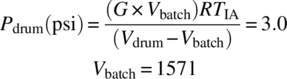
Once screening tests have determined the amount of permanent gas formed (typically in mole gas per liter, or kilogram, of batch), a preliminary assessment of the risk can be made. Assuming a certain maximum vessel fill (90%, for example) at the operating temperature, the predicted pressure rise and gas formation rate can be calculated. Comparing those values with the vessel's MAWP and/or available venting capacity, the need for more detailed evaluation of the actual hazard scenario and/or gas generation rate is warranted. For example (assuming 0.1 mol gas generated/l batch at 90% fill and 50 °C in a 100 L container), the permanent gas pressure increase in that container would be 9
- V (l) = 90 = reaction mixture volume
- Tf (K) = 323.1 = temperature
- Vh (l) = 10 = headspace volume
- R (psi·l)/(mol·K) = 1.206 = ideal gas constant
- n (mol/l) = 0.1 = gas formation
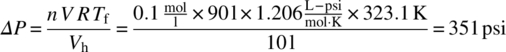
For a typical glass‐lined vessel with an MAWP of 100 psi, the above scenario is considered a potential hazard and may require a reduction in the maximum vessel fill or other mitigation such as emergency relief.
4.5 HAZARD SCENARIOS
The goal of collecting undesired decomposition reaction heat generation and gas formation data on molecules and process streams is to determine how credible it is that they pose a risk during processing. Then the consequences of risks can be assessed in an informed manner. A grid can be constructed of hazards present and the means needed to control them. See Table 4.2.
TABLE 4.2 Control Strategies vs. Hazard Sources
| No Heat | Heat | |
| No gas | Minimal or no controls needed | Temperature control to manage vapor pressure |
| Gas | Adequate venting at temperatures of concern | COMPLEX, may need pressure relief, emergency interlocks, or other advanced safety features |
4.5.1 Whole Process Overview
Once data is available on all of the key streams, it is desirable to take a holistic look at the whole process. Do any streams have exotherms that occur nowhere else in the process? Do streams before the reaction generate gas but after the reaction they do not? Does the chemistry proceed through a known unstable intermediate that might not have been captured by testing done thus far? The purpose of this exercise is to ensure that all of the possible hazards associated with a process have at least been considered and if necessary identified and evaluated.
The safety data collected will then be used to feed a hazard assessment of the process. This could be as simple as reviewing the data with the chemist running the reaction in the lab, and making them aware of any hazards, to a full PHA or HAZOP. The goal is to match both the desired process and potential process deviations with the potential consequences. Common process deviations that are considered include the following:
- Overheating (either by a jacket high temperature failure or electrical heating malfunction).
- Overcharge or undercharge of a reagent.
- Inadequate cooling during the reaction.
- Incorrect addition rate (too fast or too slow).
- Overconcentration during a distillation.
- Charging the wrong reagent or reagents in the wrong order.
- Equipment failure (controller, valve, pump, agitator).
An example for (1) might be that the vessel jacket fluid is heated via a heat exchanger that uses 180 °C steam. If there is a leak or other loss of control, the jacket fluid could reach the steam temperature of 180 °C.
How a company assesses and addresses the safety data and these deviations will be a function of a company's risk tolerance and safety posture, but there are several published papers with guidance on how to deal with these hazards [17]. The Center for Chemical Process Safety (CCPS), a division of the American Institute for Chemical Engineers (AIChE), has a good overview and extensive links to relevant material.10
The following case studies will discuss several cases where hazards were identified and evaluated against the proposed operating conditions and available safety features of the equipment. Measures were taken to either avoid encountering the hazard or make sure that the protections in place were adequate to protect the equipment and the personnel.
4.6 CASE STUDY 1: REACTION IN DIMETHYL SULFOXIDE (DMSO)
A batch process for making a pharmaceutical ingredient involved the addition of base to a pre-reaction solution composed of a brominated starting material, DMSO, and acid.
The base addition was exothermic with an adiabatic temperature rise of greater than 40 K. The batch was then heated and aged to drive the reaction forward. Gas generation was not expected, based on the stoichiometry of the desired reactions.
Review of the chemistry raised the following process safety concerns:
- The use of DMSO; a reactive solvent with a high boiling point and large exothermic decomposition at elevated temperatures [18].
- The use of DMSO in the presence of a halogen (bromine) and base [19].
Thermal screening of all process streams was carried out by DSC, while initial pressure screening of select streams [20] (starting with the end of reaction) was carried out in scanning mode using the MMC. The screen showed that there were no major process safety risks identified with the desired reactions. There was no gas generation and no exothermic decompositions of concern at the normal operating temperatures, and the exothermic base addition could be controlled by addition rate. However, consistent with the known high temperature decomposition of DMSO, DSC thermal scanning of all process streams prior to the end of reaction showed a significant exothermic decomposition (undesired reaction). See Figure 4.9. The decomposition occurs at temperatures above the normal operating temperature but is potentially reachable by a reactor jacket loss of control (overheating) process deviation, which is a single point of failure. In this case, the reactor targeted for use has a silicone‐based heat transfer fluid‐filled jacket with a maximum jacket temperature of 170 °C versus the exothermic decompositions of approximately 400–700 J/g with a DSC onset temperature of 175–225 °C. Note that the general guidance is that the EIT can be up to 50 K lower than the DSC onset temperature.
FIGURE 4.9 DSC overlay plot of process streams prior to the end of reaction. SM, starting material. The temperature was increased linearly from room temperature to 350 °C (exotherm is shown upward). Tantalum‐lined DSC cells with high pressure seals were used.
As shown by the shape of the exotherm peaks in Figure 4.9, prior to base addition the rate of the exotherm was rapid, while after the base addition the rate was much slower. Once base is charged, the presence of water in the base solution creates tempering and slows the decomposition reaction. Tempering occurs when the heat of evaporation of the solvent removes some or all of the heat generation from the decomposition.
Due to the presence of DMSO, with a freezing point of approximately 16–19 °C, DSC testing was also used to measure the potential freezing point of the stream prior to base addition (pre‐reaction stream) in order to determine if a potential deviation involves the batch freezing. Batch freezing could lead to agitation issues and lack of thermocouple reliability. A DSC scan starting at sub‐ambient temperatures confirmed that under normal operating temperatures, the batch would not freeze, as the DSC freezing point of approximately 13 °C was lower than the minimum allowable batch temperature. See Figure 4.10.
FIGURE 4.10 Pre‐reaction stream freezing point determination using sub‐ambient DSC.
In addition, due to the presence of acid, bromine species, and DMSO, a DSC was used to determine if there was a MOC impact on the undesired decomposition reaction onset, size, or rate. DSC scans of the various process streams up through base addition were performed in tantalum, Hastelloy C, and stainless steel test cells. These results were used both to assist with reactor MOC evaluation and to confirm that test results across instruments were not impacted by different MOC test cells. The DSC results using tantalum and Hastelloy C were comparable, while results for streams in stainless steel showed comparable exotherm size and onset temperature, but had a slower exotherm rate. See Figure 4.11. Therefore, data generated in tantalum and Hastelloy C test cells was considered conservative. All of the MOCs assessed are considered acceptable, but based on the slower degradation rate, stainless steel would be the preferred reactor MOC.

FIGURE 4.11 Material of construction (MOC) evaluation of pre‐reaction stream using DSC.
With thermal screening complete, the next step was to determine the pressure consequences associated with the exothermic decompositions. It was known from testing of the prior step that the exothermic decomposition in the brominated starting material had significant and rapid gas generation associated with it. ARC testing of the brominated starting material showed an EIT of 158 °C. However, the undesired activity in the brominated starting material is considered a low risk since a double upset (two deviations) would need to occur in order for this activity to be reached, a mischarge of the starting material first to the reactor with a jacket overheating deviation at that time, prior to solvent addition.
Due to the onset temperature, large size, and rapid rate of the exothermic decomposition seen in the process streams prior to base addition, the screening step for pressure consequences of these streams was skipped, and the decomposition evaluation was performed using a more advanced instrument (ARC). ARC testing was first performed on the stream prior to base addition (pre‐reaction stream), as it was likely to be the worst‐case stream for this part of the process. This was suspected to be the pre‐reaction stream based on DSC results showing that it had the lowest exotherm onset temperature, with a rapid exotherm rate. The worst‐case stream must be identified as this contains the undesired reaction for which corrective actions must be taken to either mitigate against or avoid the risks for this part of the process.
Figure 4.12 shows the plots from an ARC heat‐wait‐search conducted on the pre‐reaction stream. The heat‐wait‐search was conducted from 110 °C, at which point a series of exotherms were immediately observed, which continued to approximately 350 °C before the test was ended. Once the exotherm initiated, gas generation occurred and the pressure immediately increased. The ARC test showed that within minutes the pressure would exceed the 100 psig MAWP of the reactor, and the rupture disc would open (by 1.16x MAWP) [22]. If the rupture disc does not open or the venting capacity is inadequate then at approximately 170 °C, the maximum jacket temperature, the instruments would start failing (at 1.5x MAWP). Ten minutes later, the pressure is such that vessel failure would occur (at 3.5x MAWP). The adiabatic temperature rise associated with the first exotherm was 420 °C, and the total residual pressure (permanent gas) from the ARC test was 145 psi (at an 8 vol % test cell fill versus approximate 40 vol % vessel fill upon scale‐up). Note that DMSO boils at 189 °C, so most of the activity would be over before the temperature reaches the boiling point of the solvent.

FIGURE 4.12 Plots of temperature and pressure vs. time and pressure and temperature rate vs. temperature from an ARC heat‐wait‐search on the pre‐reaction stream conducted from 110 °C with 10°C steps and an onset threshold of 0.04 °C. A Hastelloy C ARC cell was used with a phi = 2.2. This figure is not corrected for phi; therefore the actual situation would likely be worse with a shorter time frame [21].
This first ARC heat‐wait‐search was started at 110 °C based on the DSC onset of approximately 175 °C and the general guidance that the ARC EIT can be up to 50 K lower than the DSC onset. The fact that the exotherm initiated immediately at 110 °C indicates that the actual EIT may be lower; therefore a second ARC was run starting at a lower temperature to determine the EIT of 84 °C. See Figure 4.13. In this case, the ARC EIT was greater than 50 °C from the DSC onset and did not follow the general rule of thumb; this is likely due to the fact that DMSO is a reactive solvent and the decomposition is suspected to be autocatalytic. The ARC data confirms that this exotherm is reachable by a reactor jacket loss of control (overheating) process deviation.
FIGURE 4.13 ARC heat‐wait‐search repeat run on pre‐reaction stream starting at a lower temperature to capture the EIT. A Hastelloy C ARC test cell was used with a phi = 1.4. The EIT was obtained from extrapolating to a self‐heat rate of 0.02 °C/min.
ARC testing of additional process streams, before and after the pre‐reaction stream, was completed and confirmed that the pre‐reaction stream was the worst‐case stream with the lowest EIT (see Table 4.3) and most severe pressure consequences. The higher EIT seen after the base addition is likely attributed to tempering from the presence of water.
TABLE 4.3 Exotherm Initiation Temperature (EIT) of Process Streams Prior to the End of Reaction
| Process Stream | EIT (°C) |
| DMSO + starting material | 105 |
| Pre‐reaction | 84 |
| After base addition | 144 |
Because this testing was for a multi-kilo scale process, in addition to evaluating the thermal and pressure consequences from a jacket runaway deviation, the consequences of several other credible single point of failure process deviations, identified in a hazard assessment, were investigated. None of the process deviations resulted in an exothermic decomposition worse than overheating of the pre‐reaction stream. Examples of process deviations investigated included the following:
- Missed charge of the brominated starting material.
- Undercharge of DMSO/overcharge of starting material.
- Pre‐reaction stream temperature lower than the normal operating temperature.
- Pre‐reaction stream aged for several days.
- Rapid addition of base.
- Mischarge of a more concentrated base solution.
Now that the worst‐case process stream, the pre‐reaction stream, has been identified, further testing on this stream was needed to fully characterize the exothermic decomposition. First, an ARSST experiment was run to accurately identify vent sizing parameters, as the ARSST is an open system and most closely represents the deviation at scale. Vent sizing was needed since the ARC pressure results rapidly exceed the MAWP of the vessel and indicate that the decomposition has a high likelihood of overpressurizing the vessel. From the ARSST experiment it was concluded that the system is gassy (no tempering). The ARSST also provided the temperature at which the peak pressure rate occurs, 190 °C. As shown in Figure 4.12, this was then used to predict the peak pressure rise rate of 6000 psi/min from the ARC data. In order to predict (extrapolate) the peak pressure rise rate under adiabatic conditions (phi = 1.0), a straight line was drawn to describe the effect of temperature on the pressure rise rate.
It was suspected that the undesired reaction was autocatalytic due to the sharp peak observed in the DSC and the low EIT seen in the ARC (see Section 3.5.2.3). Due to this suspicion, several 24+ hour isothermal ages were performed in the DSC in order to gain further confidence in the ARC EIT. As shown in Figure 4.14, the isothermal age at 85 °C showed an exothermic event approximately 440 minutes into the age, in alignment with the ARC EIT of 84 °C. The 65 °C and 75 °C iso‐ages showed no decomposition after 30 and 72 hours, respectively. This confirmed the temperature of concern as 84 °C.
FIGURE 4.14 DSC isothermal age overlay plot of the pre‐reaction stream aged at 65, 75, and 85 °C to gain further confidence in the ARC EIT.
With the pre‐reaction stream fully characterized, vent sizing was performed to show the consequences of reaching the undesired activity. Using the ARC/ARSST results and Design Institute for Emergency Relief Systems (DIERS) [16] vent sizing two‐phase model for a gassy system, it was determined that a vessel vent diameter of 133 cm would be needed to prevent overpressurizing the vessel, an 11 300 L reactor. This determination was based on an L/D11 of 200 versus the actual L/D of greater than 900; therefore the actual vent requirement would be even larger. As a final confirmation of the worst‐case pre‐reaction stream, vent sizing was also performed on the “DMSO+starting material” and “after base addition” streams, in addition to a rough vent sizing analysis on select process deviations; in all cases the vent sizing showed a smaller vent requirement. Since the 11 300 L reactor only had a 20 cm diameter nozzle, installing a 133 cm vent presented a major challenge; it would have required more than forty 20 cm relief vents to provide the relief area equivalent to a 133 cm vent. As this size vent is unreasonably large, a secondary vent could not be provided to protect against a vessel failure.
The above assessment identified a significant undesired reaction that could lead to vessel failure as a result of a single process deviation, reactor jacket loss of control (overheating). With all of this information in hand, a HAZOP and layers of protection analysis (LOPA) were used to determine the appropriate processing safeguards needed to mitigate the consequences and reduce the likelihood of reaching this activity to an acceptable level. In order to completely eliminate the risk, either a change in chemistry or how the process was run would be necessary.
This case study demonstrates the successful use of various calorimetric approaches to identify and characterize the thermal and pressure consequences of an undesired reaction:
- DSC for initial screening for identification of exothermic decompositions, freezing point determination, and MOC impact evaluation.
- DSC isothermal age for confirmation of the ARC EIT and verifying the suspected autocatalytic decomposition.
- ARC for EIT determination and quantification of thermal/pressure consequences to enable vent sizing.
- ARSST for determination of system type (e.g. gassy vs. tempering) and quantification of thermal/pressure consequences to enable vent sizing.
This case study also shows why reactive solvent use is discouraged, especially high boiling point solvents, as the solvent participates in the decomposition activity rather than helping to absorb heat from the decomposition. In addition, the case study shows that small changes in stream composition can greatly impact the EIT, size, and rate; for example, the pre‐reaction stream containing acid had an EIT approximately 20 °C lower than the prior stream without the acid.
4.7 CASE STUDY 2: CONTINUOUS GAS GENERATION IN A WASTE STREAM CONTAINING CARBONATE
A batch process for making an active pharmaceutical ingredient (API) involves a salt break via the addition of an aqueous 1 M potassium carbonate solution to a tosylate salt intermediate in ethyl acetate at 15–25 °C. After cutting away the first aqueous layer containing potassium tosylate, two additional washes are performed: a second aqueous potassium carbonate wash and a water wash.
Preparation of the aqueous 1 M potassium carbonate solution involves the dissolution of potassium carbonate solids, which was expected to be exothermic (~9 K) with potential minor gas generation (carbon dioxide) during initial mixing, until the pH is above approximately 8. Based on the pKa buffer curve of carbonate and carbonic acid, at pH > 8 little carbon dioxide is expected to evolve since the main component is carbonate [23].
Addition of the aqueous potassium carbonate solution to the batch was also observed to be exothermic (ΔTad < 5 K). Carbon dioxide may be generated from the potassium carbonate, but any carbon dioxide generated was expected to be dissolved in the batch stream. Since more than one mole of carbonate was present per mole of salt being broken, the main by‐products were projected to be potassium tosylate and potassium bicarbonate. However, due to the potential for carbon dioxide generation from the presence of carbonate, testing was performed to confirm if gas was being generated.
The first stream assessed for gas generation was the first aqueous potassium carbonate layer, as this stream was the most likely to generate gas and could be stored in a closed nonpressure‐rated container (e.g. drum or tank) for off‐site waste disposal. With a stream pH of approximately 8.5–9.3, carbon dioxide was not expected to evolve based on the pKa buffer curve of carbonate and carbonic acid. Using a MMC, an isothermal age (iso‐age) was performed on the first aqueous layer at 50 °C for approximately 1200 minutes (~20 hours). This temperature represents the maximum potential ambient temperature a container may be exposed to if temperature control is not provided. As shown in Figure 4.15, the iso‐age showed continuous slow gas generation.
FIGURE 4.15 MMC iso‐age of first carbonate aqueous layer at 50 °C showing continuous slow gas generation.
Due to the results on the first aqueous layer, an MMC iso‐age was also performed on the second carbonate aqueous layer. This stream had a pH of approximately 9.9–10.9. As shown in Figure 4.16, the iso‐age exhibited initial minor gas generation, but the gas generation was not sustained.
FIGURE 4.16 MMC iso‐age of second carbonate aqueous layer at 50 °C showing initial minor gas generation. But the gas generation was not sustained.
With the potential need to combine the three aqueous layers together in a vessel, an MMC iso‐age was performed on the combined stream. The combined stream had a pH of approximately 10.0. The stream was first degassed (with multiple vacuum‐pressure purges) to try to remove any potential dissolved gas. As shown in Figure 4.17, the combined stream after degassing showed continual slow gas generation, persisting from the first aqueous layer.
FIGURE 4.17 MMC iso‐age of the three aqueous layers combined at 50 °C showing continuous slow gas generation.
Due to the continuous gas generation from the first aqueous layer and the potential need to also store the organic layers in a closed nonpressure‐rated container, MMC iso‐age testing was also performed on the first organic layer (the worst‐case stream from the two carbonate washes) and the final organic stream after the water wash. As shown in Figure 4.18, the iso‐ages each showed no gas generation.
FIGURE 4.18 MMC iso‐age of the first organic layer (left) and final organic layer after water wash (right) at 50 °C showing no gas generation.
In summary, the MMC iso‐ages on the various aqueous and organic layers showed that there is a potential pressure concern with storing either the first aqueous layer or combined aqueous layers in a closed nonpressure‐rated container, while the remaining streams do not present a pressure hazard.
The rate of gas formation from the MMC iso‐age was then used to determine whether a 55 gal (208 L) poly drum containing the combined aqueous stream, which had a lower gas generation rate of 3.5 psi/day versus the first aqueous layer at 8.2 psi/day, could be safely transported off‐site for disposal. The drum was assumed to bulge if the pressure exceeded 3 psig.12
Gas generation rate calculated from MMC iso‐age (Figures 4.15 and 4.17):

Calculations showed that at a reasonable drum fill (50 vol %), the combined stream could only be stored in a closed drum for less than 2 days before the pressure reaches 3 psig and the drum begins to bulge. In order to maintain the pressure below 3 psig in the drum for 30 days, the drum fill would have to be 6 vol % (12.5 L). Due to the low drum fill requirement and short length of time leading to drum bulging, it was concluded that the combined aqueous stream cannot be stored safely in a closed drum for transport off‐site for disposal. The same is true for the first aqueous layer, as it would require even lower drum fills and shorter storage times due to the increased gas generation rate. However, at a drum fill of less than 75 vol % (157 L), the combined stream can be temporarily stored in a drum for up to 15 hours without presenting a bulging hazard (to enable necessary short‐term transportation within a site). See calculations in Appendix 4.1 at the end of this case study. A similar calculation can also be done to determine short‐term storage of the first aqueous layer.
Note that the gas generation rate does not pose a hazard for a vented vessel. This was confirmed by calculating the volumetric gas flow rate, Q, upon scale‐up in a vessel, using the MMC iso‐age gas generation rate per unit volume, Ġ. See Appendix 4.1 at the end of this case study for equation input values, except that in this case Vbatch (l) is the 10 000 L batch stream volume in the vessel:

This calculated volumetric gas flow rate is lower than a typical vessel vent capacity.
An EasyMax (by Mettler Toledo) was then used to more accurately determine the rate of gas formation during the carbonate washes. Fourier‐transform infrared (FTIR) spectroscopy was also used to confirm the gas identity, since at this time the root cause of the continuous gas generation was unknown. The experiment showed that carbon dioxide, shown by a sharp peak in the FTIR trend at 2312 cm−1, was slowly generated from the time the first charge of aqueous potassium carbonate solution is made until the first aqueous layer is cut away. The gas formation slowed down when the first aqueous layer was being settled (agitation turned off) and stopped when the second aqueous potassium carbonate charge was carried out. See Figure 4.19. In alignment with the prior MMC iso‐ages, minor carbon dioxide generation may be seen from the second aqueous layer, although the gas generation is not sustained and does not present a hazard.
FIGURE 4.19 Experiment results showing sharp carbon dioxide peak at 60 minutes once the aqueous potassium carbonate solution was added to the intermediate in ethyl acetate. At approximately 150 minutes the batch was settled, which resulted in a decrease in carbon dioxide level. Then at 210 minutes, the first aqueous layer was removed, and the second potassium carbonate wash was charged, at which point the carbon dioxide generation stopped.
As stated previously, up until this point the root cause of the continuous gas generation in the first aqueous layer was unclear. Since only the first aqueous layer continually generated gas, a closer look was taken at the tosylate salt intermediate. It was discovered that the tosylate salt intermediate may contain residual p‐toluenesulfonic acid (pTSA) from the prior processing step. Experiments were then performed to determine if the presence of pTSA with aqueous potassium carbonate and ethyl acetate would cause continuous carbon dioxide off‐gassing. A SuperCRC (by Omnical) experiment confirmed that this mixture did slowly generate pressure at a rate of 0.20 psi/h. See Figure 4.20. It was therefore concluded that the presence of pTSA with aqueous potassium carbonate and ethyl acetate does cause a slow continuous gas formation reaction.
FIGURE 4.20 SuperCRC experiment of pTSA with aqueous potassium carbonate and ethyl acetate showing slow continuous carbon dioxide generation at a rate of 0.20 psi/h.
In addition to not storing the first aqueous layer in a closed nonpressure‐rated container for off‐site transport, the first aqueous layer also cannot be sewered directly due to the contents exceeding local sewering limits for total organic carbon (TOC) [24]. Another storage option evaluated was to rent or purchase a pressure‐rated container for transport off‐site for disposal. This option was not pursued due to the high cost, long lead time, and complicated logistics. Therefore, further calorimetry experiments were carried out using an ARC, a SuperCRC, and an EasyMax (with FTIR) to determine if there was a way to stop the gas generation and enable safe storage of the first aqueous waste stream in a closed nonpressure‐rated container. Previous work already showed that degassing the layers was insufficient to remove all of the gas. Additional experiments performed included thermal treatment, raising the pH, and lowering the pH of the stream.
First it was concluded that raising the temperature of the first aqueous layer for an extended period of time did not stop the gas generation. There was still a low level of pressure generation seen in the ARC after performing a heat‐wait‐search up to 115 °C over a total exposure time of 15 hours. Then, caustic (e.g. 5 M NaOH) addition to the first aqueous layer in a SuperCRC slowed the pressure generation rate but did not stop the gas generation. Finally, addition of a strong acid (e.g. 1 M H2SO4) to an EasyMax (with FTIR) to adjust the pH of the first aqueous layer to below 4.5 (required 1 mol of H2SO4 per mole K2CO3) did successfully stop the gas generation; all carbonate was converted to carbon dioxide. The gas generation rate during the pH adjustment was directly proportional to the rate of addition of the acid. Also, the addition of acid was expected to be either mildly exothermic or potentially endothermic. It took several hours for carbon dioxide levels to decrease to zero after the acid dosing at 25 °C, likely due to mass transfer limitations as the carbon dioxide has to desorb from the aqueous phase. See Figure 4.21. It was therefore recommended to use subsurface sparging to more quickly remove the gas.

FIGURE 4.21 FTIR trend showing sharp carbon dioxide peak (at 2386 cm−1) once the strong acid is added to the first aqueous layer (shortly before 20 : 00 hours). The carbon dioxide level then dropped to zero by 24 : 00 hours.
To further confirm the above results, MMC iso‐age testing was performed on both the initial aqueous layer sample and the sample after acidic pH adjustment. The initial MMC iso‐age test showed sustained gas generation, as expected, while the MMC iso‐age test of the stream after acidic pH adjustment showed a small amount of gas generation but no sustained gas release (see Figure 4.22). This confirmed that lowering the pH of the first aqueous layer to less than 4.5 with a strong acid removes the carbon dioxide from the system and stops the gas generation in this stream, therefore making it safe to store in a closed nonpressure‐rated container.

FIGURE 4.22 MMC iso‐age at 50 °C of first carbonate aqueous layer after acidic pH adjustment to less than 4.5 showing a small amount of gas generation but no sustained gas release.
This case study demonstrates the successful use of various calorimetric approaches to identify and characterize off‐gassing of carbonate (or bicarbonate) containing streams due to the potential for gas generation, particularly if the stream may be stored in a closed nonpressure‐rated container, as this assessment will greatly reduce the potential for drum bulging incidents. It also provides an example of when it may be necessary (or desired) to perform additional operations (e.g. pH adjustment) in order to eliminate gas generation in a stream. Lastly, the case study highlights that residual quantities of materials from a prior processing step can impact downstream processing; in this case the presence of residual pTSA and its previously unknown interaction with aqueous potassium carbonate slowly generated carbon dioxide.
To determine the length of time that the combined stream can be stored in a closed drum at a 50 vol % (104 L) fill, first calculate the gas generation per unit volume in the MMC iso‐age, G:

Then calculate the gas generation rate per unit volume, Ġ:
Using a Vbatch of 104 L, solve for the number of days, X, which will result in a drum pressure of 3.0 psi by plugging in X values in the below equation until the pressure generated in the drum, Pdrum, is equal to 3.0 psi:
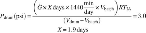
Therefore, at a drum fill of 50 vol % (104 L), the drums should not be stored for more than 1.9 days.
To determine the maximum fill level for 30‐day storage of the combined stream in a closed drum, solve for the batch stream volume in the drum, Vbatch, which will result in a drum pressure of 3.0 psi by plugging in Vbatch values in the below equation until the pressure generated in the drum, Pdrum, is equal to 3.0 psi:
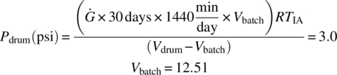
Therefore, at a drum fill of 6 vol % (12.5 L), the drums should not be stored for more than 30 days.
To determine the maximum fill level for short‐term storage of the combined stream in a closed drum, solve for the batch stream volume in the drum, Vbatch, which will result in a drum pressure of 3.0 psi by plugging in Vbatch values in the below equation until the pressure generated in the drum, Pdrum, is equal to 3.0 psi:
Note that this calculation uses the quantity of gas generated over 900 minutes of the iso‐age. Therefore, at a drum fill of 75 vol % (157 L), the drums should not be stored for more than 900 minutes or 15 hours.
4.8 CASE STUDY 3: EVALUATING A FUNCTIONAL GROUP
A research group wanted to prepare a variety of molecules containing a potentially unstable functional group (diazirine:  ). This type of molecule can upon irradiation with UV light readily form carbenes by elimination of nitrogen, making it useful in a variety of biological labeling studies [25]. Because of the potential instability from the ring strain, the research group asked for an investigation of the decomposition properties of this class of molecules.
The first compound studied was a commercially available liquid (compound 1, CAS 92367‐11‐8):  .13 The DSC on this compound (see Figure 4.23) showed an exothermic decomposition with low onset temperature (84 °C) and a large amount of energy (849 J/g).
FIGURE 4.23 DSC scan on compound 1 (CAS 92367‐11‐8) diazirine.
Based on this data, several follow‐up questions were raised that needed to be evaluated before making handling and shipping recommendations:
- Is the heat of decomposition due to the functional group only, or is there an interaction with the rest of the molecule?
- Is the decomposition different in the presence of solvents that could be used to carry out any reactions or dilutions?
- How is the decomposition affected by dilution?
- Are these compounds detonable by impact?
It was assumed that the decomposition would release 1 mol of nitrogen per mole of compound. For the compound above, for example, this corresponds to 87 ml of gas per gram of compound at 25 °C and 1 atm, which could easily produce dangerous pressures if it decomposed. This increased the importance of studying the decomposition behavior of this class of compounds.
4.8.1 Heat of Decomposition of Multiple Chemicals Sharing a Common Functional Group
From a compound collection maintained by the research group, nine different molecules, containing a wide variety of R1 and R2 non‐energetic substituents,14 were analyzed by DSC. They all gave a single decomposition peak with onset temperatures ranging from 66 to 120 °C and energies ranging from 454 to 3000 J/g. To evaluate the trend, the decomposition energy was plotted versus molecular weight (MW) (see Figure 4.24).
FIGURE 4.24 DSC energy vs. molecular weight (MW) for multiple diazirine compounds.
It was shown that a curve drawn at 320 000 (J/g) divided by the MW (g/mol) bounded the energies of decomposition. Therefore ![]() can be used as a conservative estimate of the energy of decomposition.
can be used as a conservative estimate of the energy of decomposition.
When the curves were analyzed further, in all of the decompositions where R1 and R2 were aryl or alkyl substituents, the peaks were broad like the sample compound. One compound where R1 and R2 were both part of the same ring gave a sharp peak, more typical of a potentially explosive material. As a result, any generalizations that would be drawn are limited to R1 and R2 being separate chains.
4.8.2 The Effect of Solvents
In order to make and use these compounds, they will need to be dissolved in an organic solvent, and it might be desirable to store them as dilute solutions. To see what effect several common solvents had on the diazirine functionality, DSC testing was carried out on 50% (volume/volume) solutions of compound 1 in isopropyl acetate, DMSO, and dichloromethane. (See Figure 4.25.)
FIGURE 4.25 Decomposition of compound 1 diazirine in solvents.
The results from Figure 4.25 show that the molar energy of decomposition and onset temperature were unchanged by the presence of solvent.
4.8.3 Does the Decomposition Decrease Linearly with Concentration
To support the idea that the decomposition mechanism is similar over the entire range of concentration, the commercial diazirine was tested by DSC from concentrated (100% compound) to dilute (~30 wt %) in IPAc. If there was no significant change in mechanism, the peak shape should remain the same; if the molar heat of decomposition is constant, a plot of energy per mass vs. mass fraction should give a linear plot. Based on Figures 4.26 and 4.27, the decomposition energy and mechanism is independent of concentration.
FIGURE 4.26 DSC peaks vs. concentration for compound 1.

FIGURE 4.27 Plot of energy vs. concentration of compound 1 in IPAc.
4.8.4 Is Compound 1 Detonable by Impact?
In order to ship compound 1, or any diazirine, it must not be an explosive (class 1 dangerous goods), as defined by UN regulations [26]. DSC screening of the compound can identify whether a material needs impact sensitivity testing and can help guide interpretation of the results.
As can be seen in Figure 4.23, the peak shape of the decomposition is fairly Gaussian, indicating a smooth decomposition. For comparison, the DSC of benzoyl peroxide (98%) is shown in Figure 4.28 and shows a very sharp and sudden increase in heat flow at 103 °C. This sort of change is an indicator of possible explosive properties.
FIGURE 4.28 Decomposition of 98% benzoyl peroxide.
Drop‐weight testing15 was carried out on both the benzoyl peroxide and compound 1 at 5 J of impact energy. The benzoyl peroxide gave a series of strong positive indicators of detonation at that energy level, and that particular material does have serious shipping restrictions on it (no more than 1 Lb per container for a start). Drop‐weight testing on compound 1 gave the appearance of a strong positive but closer examination of the appearance of the test cells after the runs showed that the material was not detonating, but merely decomposing. Signs included the lack of damage to a witness plate in the holder and the sample O‐ring, and the fact that the plunger was jammed in the up position, and the sample holder was hard to disassemble. When evaluated in conjunction with DSC shape, what happened was a decomposition being triggered that was slow enough that the gas formed could escape around the witness plate and lift up the plunger and wedge it in. This was verified when the holder was finally unscrewed, and large amounts of gas and liquid escaped. If a detonation had occurred, the “explosion” would have punched a hole through the witness plate, and the gas escaped through vent holes. Without the DSC evidence of a smooth decomposition, the material would have had to be classified as potentially explosive.
This difference is important, as detonations produce much more severe consequences, and can readily propagate across multiple containers. A gassy decomposition is much less severe in terms of consequences.
4.8.4.1 Thermokinetics and Safe Handling Parameters
With the DSC onset of the diazirines being between 66 and 120 °C, some questions about proper handling should be asked. Should these compounds be stored refrigerated? Are they safe to leave on the benchtop? Do they need refrigeration during shipping? With the advent of thermokinetic analysis, a series of DSC runs at different rates can be used to estimate the kinetics of decomposition without a detailed understanding of the mechanism(s). In classical kinetics it is assumed that a decomposition can be modeled by a network of reactions such as  and that each individual reaction rate equation is of the form
 ![]() . By carrying out a series of runs at different temperatures and concentrations, the rate parameters can be determined. By using a technique called “model‐free kinetics,” DSC runs at different rates can be used to estimate the rate parameters as a function merely of thermal conversion, where the model is simply
. By carrying out a series of runs at different temperatures and concentrations, the rate parameters can be determined. By using a technique called “model‐free kinetics,” DSC runs at different rates can be used to estimate the rate parameters as a function merely of thermal conversion, where the model is simply ![]() and the decomposition is treated as a single lumped reaction with the parameters a function of α, the fractional conversion.
and the decomposition is treated as a single lumped reaction with the parameters a function of α, the fractional conversion.
A new diazirine was being prepared, and it was suspected to be less stable than the benchmark compound 1. Three DSC runs at three different rates for the new diazirine as shown in Figure 4.29 demonstrated the complicated effect of changing the scan rate, and thereby the temperature–time relationship of a sample is exposed. Similar runs had been previously carried out on compound 1.
FIGURE 4.29 Effect of scan rate on DSC peak shape and size on a new diazirine.
Commercial software packages are available16,17,18 to convert these DSC curves, often in conjunction with isothermal age DSC studies and ARC runs, into an empirical model of the decomposition (and its heat generation). Once this model is available, a variety of behaviors can be predicted. For this new compound, three parameters were of particular interest. The maximum safe temperature for long‐term storage is the temperature at which 1% decomposition would take at least one month to occur. For working with the material on the benchtop, if the TMR24 was greater than 25 °C, the material would be considered sufficiently stable to handle at room temperature. The predicted SADT for a 50 kg package of the material was used to evaluate if the material needed to be classified as self‐reactive for shipping purposes and if it should be shipped cold. For this diazirine, with a 50 kg package SADT below 65 °C, UN shipping guidance [26] would state the material is a class 4.1 self‐reactive substance, and the proper shipping conditions for the actual package would need to be determined. If a 50 kg package needed to be shipped, it would need to ship under temperature‐controlled conditions with a control temperature of −12 °C [28].
Table 4.4 shows the researchers' suspicion that the new compound was less stable was correct, and it is recommended that it be held in a freezer rather than a refrigerator.
TABLE 4.4 Comparison of Properties of the Two Diazirines
| Parameter | New Diazirine | Compound 1 |
| ΔHdecomp | −590 J/g ± 50 | −890 J/g ± 30 |
| 50 kg SADT | 8 °C | 18 °C |
| tmr (25 °C) | 37.5–40 h | 57.5–60 h |
| 1% decomposition (30 days) | −10 to −5 °C | 5–10 °C |
This case study illustrates why DSC is a valuable tool for studying decompositions and understanding their behavior while requiring the preparation and use of less than 200 mg to carry out a safety assessment and guiding handling, storage, and synthesis. As a result of the DSC screening program, the research organization is now comfortable working with these highly energetic compounds.
Two additional case studies where the thermal stability of an intermediate was of practical importance for shipping and handling are shown in these articles Zhao et al. [11] and Duh et al. [29].
4.9 CASE STUDY 4: USE OF THERMAL AND PRESSURE SCREENING TOOLS TO ASSESS AN mCPBA SOLUTION
A pharmaceutical batch process involves the use of a 109 g/l solution of 3‐chloroperoxybenzoic acid (mCPBA) in a mixture of toluene and ethanol. Due to the known instability of mCPBA [30] at low temperatures and the exothermic reaction between mCPBA and ethanol, process safety testing was performed to quantify the thermal and pressure hazards associated with the solution.
Thermal screening was performed first using a DSC scan. As shown in Figure 4.30, there is a 240 J/g exotherm with an onset temperature of approximately 35 °C. This exotherm was potentially of concern because of both the large exotherm size and low onset temperature. If the exotherm was reached, decomposition would occur, and the temperature would increase approximately 120 K:
FIGURE 4.30 DSC plot of a 109 g/l mCPBA solution showing the exotherm of concern (exotherm is shown upward). The temperature was increased linearly from room temperature to 350 °C. The above plot is magnified to only show up to 200 °C; no other exothermic activity was observed in the scan to 350 °C.
A screening test was then performed using an MMC instrument to determine the pressure consequences associated with the exotherm. As shown in Figure 4.31a, in alignment with the DSC result, the MMC scan showed a 179 J/g exotherm with an onset of approximately 56 °C. There was minor permanent gas formation associated with the decomposition that resulted in a residual pressure of 2.7 psi after cooldown. See Figure 4.31b. Therefore the majority of the pressure increase during the scan was attributed to vapor pressure. Since the MMC scan did not show an obvious gas onset temperature, it was conservatively assumed that the gas formation was associated with the exothermic decomposition and had the same onset temperature as the exotherm.


FIGURE 4.31 (a) MMC scan heat generation and pressure rate vs. temperature plot for 109 g/l mCPBA solution (exotherm is shown upward). The temperature was increased linearly from room temperature to 180 °C. This plot shows the exotherm onset and size, along with the pressure generation rate. (b) MMC scan pressure vs. temperature plot for 109 g/l mCPBA solution. This plot was used to determine the residual pressure after cooldown and the pressure at maximum temperature of concern. The MMC scan was run under 16 psi of nitrogen pad gas to prevent refluxing.
The pressure data from the MMC scan was then scaled‐up to determine the consequences at large scale. Calculations were performed assuming an 80% vessel fill and a maximum temperature of concern of 413.15 K (140 °C), the maximum jacket service fluid temperature, which was also used as the worst‐case batch temperature, Tbatch:
- Vsample (ml) = 1.0 = sample volume
- Vheadspace (ml) = 1.6 = MMC cell headspace volume
- PMMC (psi) = 2.7 = residual pressure after cooldown
- Tmax (K) = 413.15 = maximum temperature of concern
- Tf (K) = 298.15 = final MMC temperature
- dP/dtmax (psi/min) = 3.3 = maximum MMC pressure rate up to Tmax
- Tbatch (K) = 413.15 = batch temperature
- R (psi·ml)/(mmol·K) = 1.206 = gas constant
- Vvessel (l) = 3785 L = total vessel volume
- Vbatch (l) = 3028 L = batch volume in vessel
First, the pressure observed in the MMC at the maximum temperature of concern was compared with the vessel MAWP to determine if there was a potential pressure hazard that may result in the safety valve/rupture disc lifting. In this case, if the mCPBA solution were to heat up to 140 °C, the pressure would be 59 psig (see Figure 4.31b and calculation below). Therefore the pressure at the maximum temperature did not pose a potential hazard when compared with a vessel MAWP of 100 psig:
The residual pressure in the vessel was then determined and compared with the vessel MAWP. This was done by first calculating the gas generation per unit volume, G, in the MMC and then using this value to calculate the residual pressure upon scale‐up, Pscale‐up, as follows:


These calculations showed that if the mCPBA solution were to heat up to 140 °C at the specified vessel fill, the 24 psig residual pressure generated did not present a potential hazard when compared with a vessel MAWP of 100 psig.
Lastly, the pressure generation rate in the vessel was compared with the vessel safety valve vent capacity to determine if there was a potential pressure hazard that may result in the safety valve lifting or equipment damage to occur. The pressure generation rate per unit volume in the MMC, Ġ, was calculated and used to determine the volumetric gas flow rate upon scale‐up, Q, as follows:
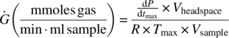
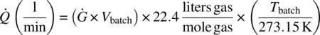
These calculations showed that if the mCPBA solution were to heat up to 140 °C at the specified batch volume, the predicted volumetric gas flow rate of 1084 L/min did not present a potential hazard when compared with a typical vessel safety valve vent capacity of greater than 30 000 L/min. Note that this calculation used the maximum dP/dt, which conservatively assumes all gas generation when in this case it is mostly vapor pressure, thus neglecting any evaporative cooling benefits.
In conclusion, pressure screening using an MMC showed that there are no potential pressure hazards associated with reaching the 240 J/g exotherm observed starting at approximately 35 °C in the DSC.
This case study demonstrates the use of a thermal screening tool (DSC) to identify a potential exotherm of concern and the use of a pressure screening tool (MMC) to conclude that the exotherm was not a hazard due to only minimal permanent pressure generation associated with the exotherm.
4.10 NOTATIONS
The common symbols used are as follows:
- Q = heat release (J/g)
- ΔH = enthalpy change (J/mol)
- Cp = heat capacity (J/g·K)
- ρ = density (g/l)
- ΔT = temperature change (K)
- ΔTad = adiabatic temperature change (K)
- T = temperature (°C)
- C = concentration (mol/l)
- ϕ (phi) = thermal inertia =
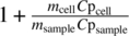 (dimensionless)
- where m = mass
- TMR24 = temperature at which the adiabatic time to maximum rate is 24 hours (°C)
- EIT = exotherm initiation temperature, typically measured in an adiabatic calorimeter such as an ARC or VSP, which is defined as a temperature rise rate of 0.02 K/min at a phi factor of 1.0. In other sources this may be referred to as the exothermic onset temperature.
ACKNOWLEDGMENTS
The author would like to thank Dan Muzzio and Don Bachert from Merck & Co., Inc., Chemical Engineering R&D Rahway, NJ 07065 USA.
REFERENCES
- 1. (a) Center for Chemical Process Safety (2008) Selection of hazard evaluation techniques, in Guidelines for Hazard Evaluation Procedures, 3rd Edition, Wiley, Hoboken, NJ. doi:https://doi.org/10.1002/9780470924891.ch6;
(b) Center for Chemical Process Safety (1995) References, in Guidelines for Chemical Reactivity Evaluation and Application to Process Design, Wiley, Hoboken, NJ. doi:https://doi.org/10.1002/9780470938058.refs;
(c) Center for Chemical Process Safety (2010) Overview of LOPA, in Layer of Protection Analysis: Simplified Process Risk Assessment, Wiley, Hoboken, NJ. doi:https://doi.org/10.1002/9780470935590.ch2; (d) Stoessel, F. (2008) Introduction to risk analysis of fine chemical processes, in Thermal Safety of Chemical Processes: Risk Assessment and Process Design, Wiley‐VCH Verlag GmbH & Co. KGaA, Weinheim, Germany. doi:https://doi.org/10.1002/9783527621606.ch1. - 2. Poje, G.V., Taylor, A.K., and Rosenthal, I. (2000). US Chemical Safety and Hazard Investigation. Report No. 1998‐06‐I‐NJ, Chemical Manufacturing Incident at Morton International, Inc., 16 August 2000. https://www.csb.gov/assets/1/20/morton_report.pdf?13798 (accessed 16 October 2018).
- 3. Perry, R.H., Green, D.W., and Maloney, J.O. (1999). Perry’s Chemical Engineering Handbook, 7the. New York: McGraw‐Hill.
- 4. ASTM E1981‐98(2012)e2 Standard Guide for Assessing Thermal Stability of Materials by Methods of Accelerating Rate Calorimetry, ASTM International, West Conshohocken, PA, 2012. www.astm.org (accessed 17 November 2017).
- 5. Hofelich, T.C. and LaBarge, M.S. (2002). On the use and misuse of detected onset temperature of calorimetric experiments for reactive chemicals. Journal of Loss Prevention in the Process Industries 15 (3): 163–168.
- 6. Crucible Brochure. Crucibles overview: DSC and TGA/SDTA. https://www.mt.com/mt_ext_files/editorial/generic/4/crucible_brochure_0x000249470002551200068070_files/51724175.pdf (accessed 29 September 2017).
- 7. Weast, R.C. (ed.) (1987). CRC Handbook of Chemistry and Physics, 68the. Boca Raton, FL: CRC Press.
- 8. ASTM E698‐16, Standard Test Method for Kinetic Parameters for Thermally Unstable Materials Using Differential Scanning Calorimetry and the Flynn/Wall/Ozawa Method, ASTM International, West Conshohocken, PA, 2016. www.astm.org (accessed 17 November 2017).
- 9. AKTS (2017). Thermokinetic Software. www.akts.com (accessed 29 September 2017).
- 10. Yoshida, T., Yoshizawa, F., Itoh, M. et al. (1987). Prediction of fire and explosion hazards of reactive chemicals. I. Estimation of explosive properties of self‐reactive chemicals from SC‐DSC data. Kogyo Kayaku 48 (5): 311–316.
- 11. Zhao, R., Muzzio, D., Vickery, T. et al. (2018). Thermal hazard investigation of a pharmaceutical intermediate. Process Safety Progress 37 (2): 263–267. https://doi.org/10.1002/prs.11917.
- 12. Singh, J. and Simms, C. (2001). The thermal screening unit (TSU) a tool for reactive chemical screening. In: Hazards XVI, IChemE Symposium Series, vol. 148 (ed. Institution of Chemical Engineers). Rugby: Institution of Chemical Engineers.
- 13. Thermal Hazard Technology (THT), Rapid Screening Device (RSD) A cost‐effective calorimeter for screening samples for exothermic reaction hazards. www.thtuk.com (accessed 29 September 2017).
- 14. NETZSCH. Multiple mode calorimetry (MMC). https://www.netzsch‐thermal‐analysis.com/en/products‐solutions/multiple‐mode‐calorimetry (accessed 29 September 2017).
- 15. Burelbach, J.P. (2000). Advanced reactive system screening tool (ARSST). Presented at the 28th Annual North American Thermal Analysis Society (NATAS) Conference, Orlando, FL, (4–6 October 2000).
- 16. Fisher, H. G., Forrest, H. S., Grossel, S. S., Huff, J. E., Muller, A. R., Noronha, J. A., Shaw, D. A. and Tilley, B. J. (1993) Front matter, in Emergency Relief System Design Using DIERS Technology: The Design Institute for Emergency Relief Systems (DIERS) Project Manual, Wiley, Hoboken, NJ. doi:https://doi.org/10.1002/9780470938317.fmatter.
- 17. Fauske, H.K. (2006). Managing chemical reactivity: minimum best practice. Process Safety Progress 25: 120–129. https://doi.org/10.1002/prs.10126.
- 18. (a) Lam, T.T., Vickery, T., and Tuma, L. (2006). Thermal hazards and safe scale‐up of reactions containing dimethyl sulfoxide. Journal of Thermal Analysis and Calorimetry 85 (1): 25–30. (b) Wang, Z., Richter, S.M., Gates, B.D., and Grieme, T.A. (2012). Safety concerns in a pharmaceutical manufacturing process using dimethyl sulfoxide (DMSO) as a solvent. Organic Process Research & Development 16 (12): 1994–2000. https://doi.org/10.1021/op300016m. (c)Brandes, B.T. and Smith, D.K. (2016). Calorimetric study of the exothermic decomposition of dimethyl sulfoxide. Process Safety Progress 35: 374–391. https://doi.org/10.1002/prs.11802.
- 19. Bassan, E., Ruck, R.T., Dienemann, E. et al. (2013). Merck’s reaction review policy: an exercise in process safety. Organic Process Research & Development 17 (12): 1611–1616. https://doi.org/10.1021/op4002033.
- 20. Frurip, D.J. (2008). Selection of the proper calorimetric test strategy in reactive chemicals hazard evaluation. Organic Process Research & Development 12 (6): 1287–1292. https://doi.org/10.1021/op800121x.
- 21. Townsend, D.I. and Tou, J.C. (1980). Thermal hazard evaluation by an accelerating rate calorimeter. Thermochimica Acta 37 (1): 1–30. https://doi.org/10.1016/0040‐6031(80)85001‐5.
- 22. (a) ASME ASME Boiler and Pressure Vessel Code, Section VIII Pressure Vessels, Division 1. New York, NY: American Society of Mechanical Engineers http://www.asme.org/shop/standards/new‐releases/boiler‐pressure‐vessel‐code‐2013. (b) Crowl, D.A. and Tippler, S.A. (2013). Sizing pressure‐relief devices. Chemical Engineering Progress 109: 68–76. (c) Sandler, H.J. and Luckiewicz, E.T. (1993). Practical Process Engineering. New York: McGrew‐Hill.
- 23. International Atomic Energy Agency (IAEA). Environmental isotopes in the hydrological cycle: Vol. 1, Ch. 9 pg 94, Figure 9.6. http://www‐naweb.iaea.org/napc/ih/documents/global_cycle/Environmental%20Isotopes%20in%20the%20Hydrological%20Cycle%20Vol%201.pdf (Accessed 18 October 2018).
- 24. Environmental Protection Agency (EPA) (1990). Environmental protection agency land disposal restrictions for the third third scheduled wastes. Federal Register 55 (106), 1 June 1990. https://www.epa.gov/sites/production/files/2016‐02/documents/55_fr_22519_to_22720_june_1_1990_thirdthird.pdf (accessed 17 November 2017).
- 25. Dubinsky, L., Krom, B.P., and Meijler, M.M. (2012). Diazirine based photoaffinity labeling. Bioorganic & Medicinal Chemistry 20 (2): 554–570. https://doi.org/10.1016/j.bmc.2011.06.066.
- 26. United Nations (1999). Recommendations on the Transport of Dangerous Goods, Third Revised. New York: United Nation.
- 27. ASTM E680‐79(2011)e1 (2011). Standard Test Method for Drop Weight Impact Sensitivity of Solid‐Phase Hazardous Materials. West Conshohocken, PA: ASTM International.
- 28. US Department of Transportation Title 49 (2011). Code of Federal Regulations on Forbidden materials and packages. https://www.gpo.gov/fdsys/pkg/CFR‐2011‐title49‐vol2/pdf/CFR‐2011‐title49‐vol2‐sec173‐21.pdf (accessed 17 November 2017).
- 29. Duh, Y.S., Yo, J.M., Lee, W.L. et al. (2014). Thermal decompositions of dialkyl peroxides studied by DSC. J. Therm. Anal. Calorim. 118: 339.
- 30. Sigma Aldrich Corporation (2018). Safety Data Sheet (SDS) for mCPBA. http://www.sigmaaldrich.com/MSDS/MSDS/DisplayMSDSPage.do?country=US&language=en&productNumber=273031 (accessed 2 March 2018).