
15
DEVELOPMENT AND APPLICATION OF CONTINUOUS PROCESSES FOR THE INTERMEDIATES AND ACTIVE PHARMACEUTICAL INGREDIENTS
Flavien Susanne
Product and Process Engineering, GSK Medicines Research Centre, GlaxoSmithKline, Stevenage, UK
15.1 INTRODUCTION
Continuous process operation is a manufacturing methodology that dominates the production of bulk chemicals. It is seen as the method of choice for delivering products associated with the oil and gas, food, and polymer industries. The process operations of such industries are driven by allowing consistency of the quality, enabling high demands and predominantly lowering the cost of goods (CoGs); positive margins can be achieved from low value raw materials and products. In contrast, the pharmaceutical industry has not placed much focus on the manufacturing cost of their final products, drug substance (DS) and drug product (DP) as, until recently, these were considered high value products with an extremely high margin. However, in the last 10–15 years, the emergence of generic companies,1 manufacturing off‐patent drugs in parts of the world where there are lower labor and overhead costs, has reduced the revenues of the pharmaceutical companies’ overall.
Active pharmaceutical ingredient (API) manufacture involves low volumes, where demand is uncertain. Therefore, API manufacture had traditionally been in the domain of versatile and multipurpose batch manufacture, which remains the mainstay of the pharmaceutical industry. Pharmaceutical companies are now being forced to adjust their business models to react to generic competition. Enhanced value brought by new technologies is seen as the direction forward. We now see among process transformation the emergence of enzymatic transformations, specific catalytic transformations, and high value continuous processing. In the past decade, there has been a growing interest in the application of continuous processing in the pharmaceutical industry for two reasons. Firstly, flow chemistry enables a diversity of reactions from which to synthesize a molecule [1, 2]. Such approaches facilitate the synthetic route to a molecule that may in turn produce a simpler manufacturing process. Secondly, a rationale has emerged based around factory or supply chain benefit. This approach argues that telescoping multiple synthetic steps together in a continuous supply chain leads to benefits including reducing inventories and allowing more responsiveness to product demand [3].
Only recently have continuous processes started being implemented into pilot plant and small‐scale manufacturing facilities. Most of these recent examples are predominantly single‐stage processing for chemistry‐enabling applications where a mass and heat transfer problem needs to be solved or controlled. With progressive innovation and development of new technologies, drug development and production is expected to move toward lower volume, customized, or patient‐specific drugs. This trend of manufacturing many new (and low volume) products will force the pharmaceutical industry to improve drug quality yet at reduced manufacturing cost, which accounts for 36% of total industry cost [4]. In the recent years, given the pressure of cost reduction, improved consistency in DS or DP quality, and enhanced manufacturability, the design of multistep continuous manufacturing has emerged as a promising solution to address most of these constraints.
The response from the pharmaceutical industry cannot be a simple transfer of technology used in other industries. While oil and gas or polymer product volumes represent extremely high tonnage per annum, API volumes rarely exceed 100 metric tons per annum, with an obvious trend leading toward smaller volumes in the future due to high efficiency and potency drugs.
Implementing continuous processing in the pharmaceutical industry is not trivial. It is often the answer when solving complex problems. Due to the high complexity of the chemical transformations, including intricate pathways from the starting materials to the product and a high number and diversity of impurities to be controlled to precise level, continuous process development requires the solving of interlinked chemical and engineering problems. To enable the efficient implementation of continuous process into the pharmaceutical world, the approach of process development and scale‐up, first, has to be reassessed. Until recently, the pharmaceutical industry has relied on chemistry knowledge to bring their drugs from candidate selection to manufacture. For the development of continuous processing, the merging of multiple skill sets is necessary, complementing chemistry expertise with engineering application as part of the process design. Continuous process development involves generating deep process understanding across each unit operation. Together, kinetic and thermodynamic process models of the unit operations are generated including physical rates and performance of the process equipment. Understanding the intricate mechanisms taking place between the chemistry and the technology is key to the design, as it enables optimization and process transfer to manufacture in the most efficient way.
15.2 VALUE OF CONTINUOUS PROCESSES FOR THE PHARMACEUTICAL INDUSTRY
15.2.1 Access to a New Range of Operational Conditions and Transformations
Traditionally, due to the batch technology being used, process operation in the pharmaceutical industry is limited to a narrow range of pressure, temperature, and reactivity. Despite the benefit of such vessels in terms of flexibility and versatility to perform a recipe, they are limited in the range of conditions, which they could achieve in terms of pressure and temperature. In addition, due to their size, geometry, design, and poor surface to volume ratio, such vessels provide limited efficiency of heat and mass transfer. Therefore, the way processes could be operated becomes restricted, and generally processes do not achieve full optimization.
In contrast, continuous process technologies are made to enhance all physical rates such as heat and mass transfer. Smaller size technology enables an increase of the heat transfer coefficient, surface to volume ratio, and high efficiency of fluid dynamic. By increasing the operating space, less conventional chemistry can now be explored within a wider range of conditions. Process optimization can be extended toward new boundaries no longer limited by a narrow range of operations dictated by the large manufacturing vessels. The process conditions such as pressure, temperature, reaction time, or stoichiometry can be tuned more easily to reach optimum process output. In addition, transformations requiring high pressure and high temperature, such as Claisen, Cope, or Fisher indole rearrangement, can now be industrialized for manufacturing demand [2].
New types of transformation are now being explored with some success, among them photochemistry and electrochemistry. Photochemistry, despite its great potential, was limited until now by the light penetration depth and the photon exposition achieved in a big batch vessel. Therefore, photochemistry never broke through, as no scale‐up pathway was identified. With the development of continuous technology with high surface to volume ratio see‐through reactors and efficient penetration of the photon, simplified access and scale‐up of photochemistry have become possible.
15.2.2 Safety of Operation
Operation in pharmaceutical manufacture has often been limited by the efficiency of the technology in place. We can find two classes of reaction where, to enable operations to be performed in a safe manner, processes are suboptimized and efficiency is needed to be compromised.
The first class of reaction is fast and/or exothermic; the poor mass and heat transfer achieved in big batch vessels forced these processes to be operated as dose‐controlled addition to keep the heat release under control. From literature, a large range of examples such as nitro reduction, organometallic, or oxidation transformations could be found where suboptimum processes must be implemented in manufacture to keep them safe [5, 6]. These transformations have the specificity to generate extremely high exotherm, up to 1000s of kJ/mol and an extremely high adiabatic temperature raise, above 300–400 °C in some cases.
The second class of reaction can be defined by unstable and/or explosive intermediates, triggering the possibility of generating uncontrolled runaway reactions. The slow dynamic of large batch vessels forces these processes to be operated, predominantly, as dose‐controlled addition, conditions far from their kinetic optimum to prevent accumulation. In the pharmaceutical industry, a safety margin of 50 °C is often applied from any onset of decomposition, to ensure safe operation. Reactions that are commonly found in API synthetic routes such as Curtius, nitration, or oxidation reactions are then underperformed [7, 8].
By enhancement of the heat and mass transfer, the use of continuous technology enables a more precise control of the process parameters and a much faster response to changes ensuring safe operation. The heat released by these reactions, or thermal instability, becomes easier to control by the high heat transfer coefficient and surface to volume ratio of the continuous technology. In some cases, such as peroxide oxidation, the process is operated in flow significantly above the onset of the reagent decomposition as the safety is achieved through an understanding of the relative rates of decomposition versus main reaction.
15.2.3 Quality Control
In the pharmaceutical industry, high quality of the finished product is mandatory. DS and DP are defined with extremely high quality specifications. However, the inaccuracy and lack of reproducibility of large batch processing generates out of specification material on a regular basis. This material can either be reprocessed or sometimes completely discarded from the chain of supply. Such defects, due to the high cost of raw materials and labor and overhead, have a significant negative impact on the overall cost of a drug.
Continuous processing by implementing tight controls of the process parameters and highly responsive process control and by minimizing manual intervention removes a significant number of the variables triggering poor quality material. A more consistent high quality end product can be achieved during state of control operations. The process is often monitored using various soft sensors and process analytical technologies. The quality output of the material can be achieved using two approaches. The first, closely related to batch philosophy, links the process input reading to a predefined output using design spaces. When disturbances are observed and the process parameters exceed the acceptance limit, the material is diverted and quarantined. The second one, more aligned with the philosophy applied in other industries such as bulk chemicals or oil and gas, looks at implementation of model predictive control (MPC). The process inputs are processed through a series of linear or nonlinear models to correct disturbances by applying feedback and feedforward counteractive measures.
15.2.4 Reduction of Cost
Most pharmaceutical industries are still focusing on the technical value that continuously can provide to their company. However, few pharmaceutical companies are now moving toward developing and integrating continuous multistep processes into their manufacturing facilities. For those processes, the implementation of new technology can be aligned with the integration of a concept‐based recipe with a high degree of automation of the process operations. In addition, as defined in the quality control section above, process control can be achieved using more advanced process control such as MPC. The manual operation becomes minimal. The direct impact is the reduction of labor and overhead costs. However, as most process variation of material quality output is mainly related to human intervention or error, automated procedures allow significant opportunity for improvements in robustness and reproducibility. Less defects are then observed leading to less reprocessing or rejection of the final product.
Such an approach of automating and controlling processes using feedback and feedforward is well established in other industries such as the oil and gas or the tobacco manufactures. Those industries operate at a much greater sigma level than the pharmaceutical industry, enabling a significant overall CoGs reduction.
15.3 CONTINUOUS PROCESS DEVELOPMENT WORKFLOW
Continuous process development and scale‐up into manufacturing facilities are not necessarily trivial. As described in Section 15.2, continuous processing is implemented to tackle considerations of quality control and safety, for highly demanding mass and heat transfer during chemical transformations. Therefore, continuous processing requires a detailed process understanding to ensure appropriate operating condition definitions, equipment design, and process control. Efficient continuous process development and scale‐up are based on a workflow, where process understanding and equipment performance are combined through process modeling (Figure 15.1). Process simulation acts as a platform centralizing all process information, enabling holistic process definition and optimization.
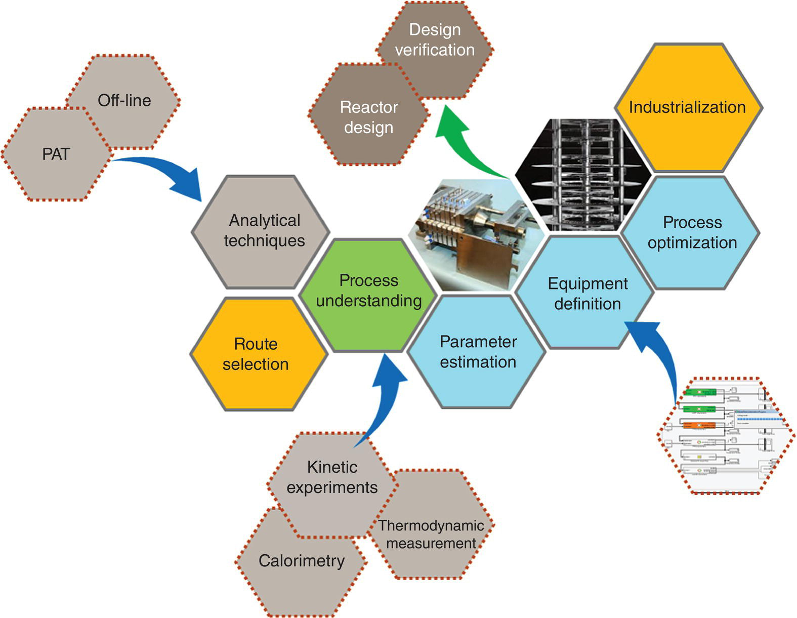
FIGURE 15.1 Schematic of the various phases of continuous process development.
The process understanding workflow can be applied similarly to all unit operations; however, the methodology will be exemplified using reactions in the following sections.
15.3.1 Process Understanding
Regardless of the type of unit operation considered, a process is defined by its energy and mass balance. The process understanding described below is focusing on providing all critical information; enabling the definition, the optimization of the process, and further linking with equipment performance.
15.3.1.1 Energy Balance
Often for batch processes, the energy balance is neglected during the early process development activities and only integrated toward the end, to ensure safe operation during scale‐up. The reverse is true for continuous process development; the understanding of the energy balance is considered critical to process design. The transfer of highly exothermic processes to continuous operation and the optimization can be challenging due to the overall heat and rate of release. Therefore, a tight control of the process parameters is required to ensure safe operation and quality attribute of the product. Being able to map out the enthalpy related to each major aspects of the process is critical. Across the process, the enthalpy of reactions, dissolution, crystallization, mixing, and evaporation are summed up as a function of their rates to provide a dynamic picture of the process energy.
Techniques to measure enthalpies are not specific to batch or flow; classic batch calorimeters such as RC1, adiabatic accelerating rate calorimetry (ARC), and differential scanning calorimetry (DCS) [9–12] where the enthalpy is calculated from the integration of the overall heat flow can equally be used for flow. Heat flow traces of any investigated reactions can be gathered by measurements of non‐isothermal or isothermal conditions. Despite their mode of operation and slow dynamic, they provide crucial information regarding the enthalpy of each single operation, even for flow operation. Batch calorimeters are limited in their function when fast and energetic reactions need to be assessed. In those cases, rates are impossible to regress as the heat released is limited by physical rates such as dosage. However, when the operation analyzed is not limited by the dynamic of the batch calorimeter, in addition to the heat flow, estimation of rate constants (k) and activation energy (Ea) can be achieved.
The reaction considered in the example illustrated in Figure 15.2, where A reacts with B forming product C, is followed by a by‐product formation D and decomposition to form E. The heat flow measurements allow the overall heat released to be obtained where each reaction contributes in a certain specific ratio to the total observed heat flow. From the integration of the overall heat of reaction (Qr), the enthalpy of reactions (ΔHr), the rate constant (k), and activation energy (Ea) of each transformation can be calculated using expression (15.1) and the methods described below [10]:
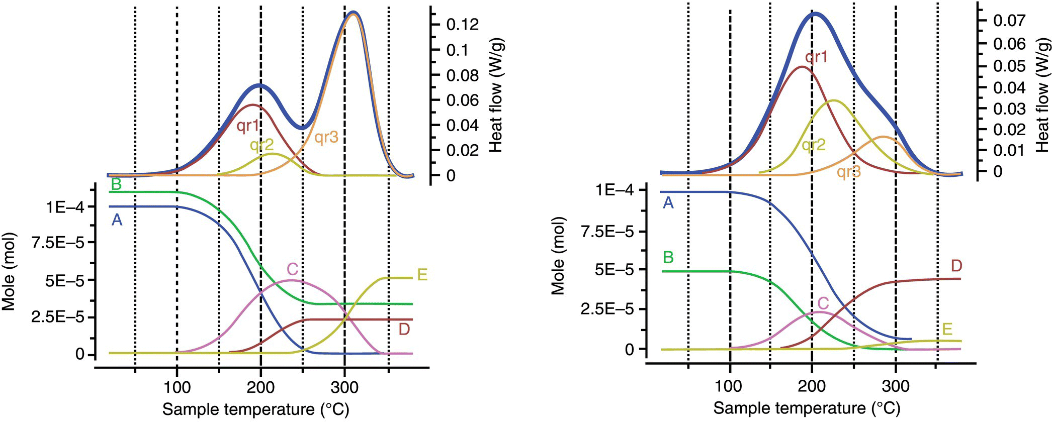
FIGURE 15.2 Heat flow signals and reagent profiles obtained by DSC under non‐isothermal conditions, heating rate of 2 K/min; stoichiometry excess of 1.1 equiv. of B over A (left), sub‐stoichiometric of 0.5 equiv. of B over A (right).
Two methods have been developed and commonly used to regress kinetic parameters from heat flow. The first method, the Borchardt and Daniels kinetics approach, allows the calculation of activation energy (Ea), pre‐exponential factor (k0, r), heat of reaction (ΔHr), and reaction order (n) from a single DSC scan [12]. The kinetic approach is based on Eq. (15.2):
The equation above can be solved with a multiple linear regression of the general form k0,r where the two basic parameters, ∂[A]/∂t and α, are determined from the DSC exotherm as shown in the DSC (Figure 15.2). This approach requires only a single temperature programmed experiment. This makes the approach highly attractive.
The second method, the ASTM E698 approach, is based on the variable program rate method of Ozawa, which requires a minimum of three DSC scans at different heating rates, usually between 1 and 10 °C/min [13]. The method assumes that the conversion at the peak exotherm is constant and independent of heating rate. By plotting ln k versus 1/T, calculation of the activation energy (Ea) and pre‐exponential factor (k0,r) can be achieved. The ASTM E698 shows great accuracy on the regression of the activation energy, but the pre‐exponential factor (k0,r) may not be valid since the calculation of k assumes a reaction order predefined. However, the ASTM method is often the only means to analyze reactions with multiple exotherms [14].
Following the successful parameter estimation of the reactions using the methods described above, the evolution of the process can be expressed as molar time course profile where depletion and formation of the components A, B, C, D, and E are shown. Such model can be used for the prediction of any conditions and scenarios: isothermal, isoperibolic (constant temperature of the heat exchanger), adiabatic (cooling failure), and runway.
In the cases of fast reactions with unstable intermediates or competitive pathways, the use of traditional batch calorimeters to provide time‐relevant information becomes limited. To prevent approximation in the energy balance calculation between the reaction studied and various parallel decompositions, some universities have been working on the design of flow calorimeters, allowing a better measurement of the heat flow for sub‐minute reaction time. So far, the design of these new devices remains within the hand of academic groups with no real commercial equipment being available soon.
15.3.1.2 Mass Balance
It was shown on the section above that calorimetry data could be used not only for calculation of enthalpy of reactions but also to regress other kinetic parameters such as rate constants and activation energies. However, these techniques show limited sensitivity, and the possibility to decouple all the phenomena taking place at the same time can be difficult to achieve. Therefore, for the process understanding of reactions, in addition to the energy balance and calorimetry data, molar time course profiles are often generated. Conventionally, they are generated at various concentrations and temperature mostly under isothermal conditions; however, non‐isothermal profile can be applied [15]. They comprehend the major components of the mass balance such as starting materials, reagents, products, and major side products. The molar time course profile is sometime extended to critical impurities called critical quality attributes (CQAs) when the control of their formation is deemed to be important to the API.
With the difference from other industries where kinetic understanding is often limited to the understanding of a single, even complex, transformation, e.g. continuous hydrogenation in the oil and gas industry or polymerization in the polymer industry, the pharmaceutical industry is often working on the synthesis of new molecules involving reaction of building blocks never seen before. The transformation pathway is not always well defined, and a large range of new impurities appear. The control of those impurities to a low level, often below 0.1% w/w, is critical to the attribute of the final product and its commercialization. Generating mechanistic understanding of such complex transformations is challenging but highly valuable as it enables the definition and the optimization of the process in respect of the control of those impurities.
15.3.2 Laboratory Equipment
15.3.2.1 Mesoscale Reactors
To conduct the process understanding activities of continuous processes, small batch equipment is often used. We can find in the pharmaceutical laboratories a wide range of well characterized and automated small batch platforms [16]. However, even if they can cover a large range of process conditions, laboratory batch reactors are limited by their heat and mass transfer performance. As continuous process opens and stretches the ranges of operation, looking at sub‐second transformations, high temperature, and high pressure conditions, the technology to study these transformations needed to align with this new intent. To answer these new needs, we saw in the last 10 years the emergence of meso‐reactors and fast new analytical techniques [17, 18]. Both are the specific examples where technologies have been designed to enhance process understanding.
Meso‐reactor designs took in consideration the enhancement of both aspects of mass and heat transfer. Such systems demonstrate the capability to achieve very high heat transfer coefficient due to an astonishing high surface to volume ratio and a very low mass ratio between the process media and the thermomass of reactor system itself. In addition to the temperature control, some special attentions from the mesoscale supplier technologies went on the mixing elements and sizing of the capillary to ensure really fast micromixing time and very high Bodenstein number [19]. Few suppliers are now providing an array of meso‐reactors and mixers in different materials of construction – hastelloy, stainless steel, silicon carbide, or glass with various geometries – and sizes to accommodate the range of chemistry seen in the pharmaceutical industry (Figure 15.3).2–5

FIGURE 15.3 Examples of various meso‐reactors available off the shelves.
In addition to the work done by the suppliers, few academic groups worked on the characterization and the utilization of this new range of microfluidic mixers and reactors [20–23]. A specific example where meso‐reactors pushed the boundary of process understanding is the development of segmented flow systems (Figure 15.4). The capillary and wetting forces enabled the enhancement of the mass transfer. In these systems, through an extensive organic film deposition on the walls of the reactor, a large specific surface area for the dissolution of the gas into the organic phase is generated. The concentration of dissolved gas at the gas–liquid interface can be assumed to be equal to the gas solubility. In addition, as the width of the organic segment is significantly smaller than the inner diameter (ID) of the reactor, internal convection could be considered inexistent, and mass transfer is driven by diffusion only. Therefore, a simple film theory‐based treatment of transport and reaction is applicable. Despite the nature of the multiphase system studied in this type of reactor, a tremendous acceleration of the mass transfer phenomenon is observed enabling opportunity to study intrinsic kinetics, which could not be achieved previously.
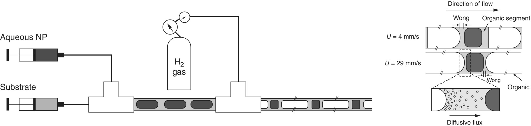
FIGURE 15.4 Schematic illustrating the mass transfer of dissolved reactants in the triphasic segmented flow.
Source: Courtesy of Saif Khan, National University of Singapore.
15.3.2.2 In‐line, Online PAT
The pharmaceutical industry is already using a large array of process analytical technology (PAT) to measure in situ evolution of processes. Mid‐IR, Raman, or UV instruments are now commonly spread across development and manufacturing. However, the type of probe used and their response time are not appropriate to continuous processing applications. New and fast analytical technologies have been developed in the recent years to support the understanding of continuous processes. Extremely fast reactions can be a challenge for their monitoring using traditional off‐line method; therefore, generating intrinsic understanding of these reactions is limited. Suppliers invested time in the development of new PAT and flow cells, enabling the process understanding and development of continuous processes by collecting compositional information.6,7
Equally, NMR suppliers adapted their technology to respond to the new requirement of continuous process understanding. Complex and new design NMR flow cells and low‐field NMR benchtop are now available.8,9 The reworking done on the NMR spectrometer now allows minimum calibration and the use of non‐deuterated solvents. Two modes of usage are currently possible (Figure 15.5), either by circulating reacting materials from an external reactor through the magnet for rapid spectral acquisition, thereby enabling online monitoring, or by in situ measurements where reagents are mixed directly inside the magnet. This enables measurement of the kinetics of fast reactions.

FIGURE 15.5 Schematic illustrating the application of online and in‐line NMR spectrometer for process understanding.
Source: Courtesy of Anna Codina, Bruker.
More standard technologies, traditionally used as off‐line method are now transitioning to in‐line or online PAT. With the support of suppliers, pharmaceutical research and development and academic groups are repurposing LC, MS, and GC instruments to online systems where major and low‐level components could be quantified. Not only are those PATs of interest for process understanding, but they are also finding their way to pilot and manufacturing facilities to ensure compliance of the product, preventing long and costly traditional in‐process control (IPC) analysis and batch defect.
Using some of the technology described above, either standard batch or mesoscale reactor, combined with new PAT technologies, molar time course profiles can easily and reliably be generated. Process understanding of complex and fast reactions that remained in the hands of specialized academic groups in the past can now be studied in the pharmaceutical laboratories.
15.3.3 Parameter Estimation
For the application of reactions, process model is used as a platform to describe the various transformations through a matrix of differential rate equations. However, due to the complexity and diversity of processes, the definition of the transformation map feeding the model is often iterative and rarely right first time. These rates expressions often include enthalpy of reaction, pre‐exponential factor, constant of equilibrium, and activation energy. Using the calorimetry data and the molar time course profiles generated at different input concentrations and temperatures during the process understanding phase of development, the kinetic parameters of each individual transformation can be estimated. The traditional way of using the Arrhenius plots, linearization of ln(k) against 1/T, can be applied. However, with the increase of computing power and emergence of simulation software, the estimation of the kinetic parameters can be simplified using the expressions (15.3 and 15.4) in dynamic kinetic models by performing the regression of all parameters simultaneously.
Comparing the experimental data with the model predictions allows a constant refinement of the mechanistic proposal until acceptable agreement between the model prediction and the data (Figure 15.6).
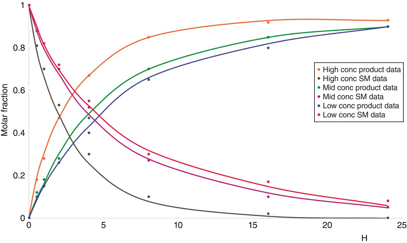

FIGURE 15.6 Kinetic parameter estimation at various temperatures and concentrations. Dots are experimental data as the trends are the predictions provided by the software after fitting of the pre‐exponential factors and the activation energy.
When satisfactory prediction has finally been achieved, verification of the model using an additional set of experiments is usually performed. These experiments must be within the same ranges of conditions used for the parameter estimation as the model should not be used for extrapolation. The set of experiments used to verify the model is defined, using sensitivity analysis tools, as a function of the process sensitivity against the input parameters. It often happens that the verification experiments are grouped within a specific part of the process parameter ranges as the response is greater in this region (Figure 15.7).
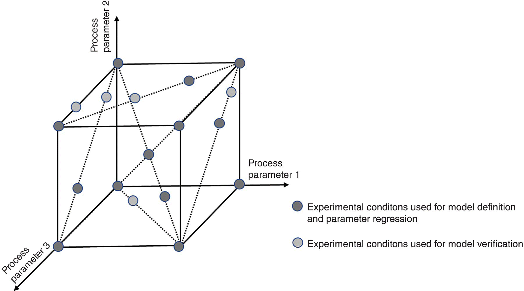
FIGURE 15.7 Graphical representation of a set of experiments used for model definition and model verification.
When the verification is complete and successful, the model can be used within the range of conditions defined as a predictive tool to evaluate impact of process parameters to yield and process quality.
15.3.4 Equipment Performance
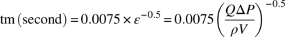
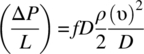
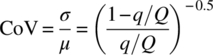
Having a detailed understanding of the equipment performance is critical for continuous processing as it allows to properly understand the process output in respect to the technology. Two physical rates are often seen important to the process: the micromixing (tm in second) [24], which could be calculated using standard dissipation energy and pressure drop in pipes or the coefficient of variation (CoV) [25, 26], or macromixing homogeneity, defined as the ratio of the standard deviation (σ) to the mean (μ). The axial dispersion referred the dimensionless Bodenstein number (Bo) [27] and the heat transfer coefficient (U in W/m2∙K). At first, mathematical expressions (15.5)–(15.11) can be used to estimate these physical rates and evaluate the sensitivity of the process against them:
ΔP for turbulence regime in cylindrical pipe:
ΔP for laminar regime in cylindrical pipe:

where q is the minor volumetric flow rate and Q the major volumetric flow rate:

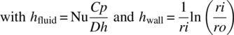
For a low‐energy release processes, an estimation of the heat transfer coefficient and wetted area (UA) based on the dimensionless number of Reynolds (Re), Nusselt (Nu), and Prandtl (Pr), reflecting the flow velocity, the physical properties of the process media, and the heat transfer fluid (HTF), the thickness, and conductivity of the material of construction can be estimated with reasonable accuracy. A similar approach with the mass transfer, e.g. macromixing and the axial dispersion, should be applied. Initial calculations based on the design of the reactor allow calculations of the blending time between two streams using the CoV or tm and the calculation of equivalent number of reactor using Bo mathematical expressions. If further accuracy is required as the sensitivity of the process is high in respect of any of these physical rates, they could be accurately measured using well‐defined procedures.
A comprehensive definition of UA using the Sieder–Tate correlation can be conducted using Eqs. (15.11)–(15.15).
Nu for laminar flow:
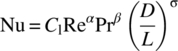
where α, β, and σ could be estimated to 0.33 and Cl to 1.86
Nu for turbulent flow:
where α and β could be estimated, respectively, to 0.8 and 0.4 and Ct to 0.023:
However, these expressions can be further refined by estimation of these exponent coefficients through a regression of heat up and cool down temperature profiles. Such estimate will allow greater heat balance prediction sensitivity for process with high exotherm and non‐isothermal processes with large delta of temperature [26].
To increase the accuracy of the measurement of the temperature across the length of the reactor, new sensors have emerged. We now can use multiple thermocouple device positioned across the length of the reactor providing up to one measurement every centimeter. However, more recently, fiber optics have been used for the same application, and a measurement every 20 nm is now achievable. The generation of such temperature profiles provides valuable and reliable information to regress the U value.
For meso‐reactor, where direct measurement of the temperature is not feasible, a new innovative methodology has been tested with success. For see‐through reactors, for example, procedures using quant dot where the dot emits a different color depending of their temperature have been implemented to characterize the U value of those highly efficient reactors [28]. For metal reactors, procedures using reactions with high activation energy can be used as the quality output is directly related to the temperature profile into the reactor and therefore the heat transfers. Among them, we can find a library of Diels–Alder reaction [12].
The Bodenstein number or axial dispersion coefficient can be easily measured using residence time distribution (RTD) procedures. Two types of measuring the probability distribution function and comparing to the ideal behavior are readily available, the Dirac pulse and the step change methods. The coefficient is calculated by measuring the variance (δ) between the input and output signals.
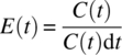
The Dirac pulse method is based on the introduction of a very small volume of a tracer at the inlet of the reactor over a short and controlled time. The concentration over time resulting curve C(t), can be transformed into a dimensionless RTD curve, E(t), by the following relation (15.8):
The step method is based on the introduction of an abrupt change from 0 to C0 of a tracer at the inlet of the reactor. The concentration of tracer at the outlet is measured and normalized to the concentration C0 to obtain the nondimensional curve F(t), which goes from 0 to 1 and then transformed into a dimensionless RTD curve E(t) (Eq. 15.17):
An ideal plug flow reactor (PFR), where each component enters and leaves in the exact same order, has a variance (δ) of zero, E(t) = δ(t − τ). As the behavior of the reactor deviates from ideal PFR, the variance increases toward the behavior of a continuous stirred tank reactor (CSTR) system E(t) = 1/τe(−t/τ) with a variance (δ) of ∞. The variance can be equally referred as equivalence of reactor n, from n = ∞ for ideal PFR to n = 1 for ideal CSTR [29] (Figure 15.8).
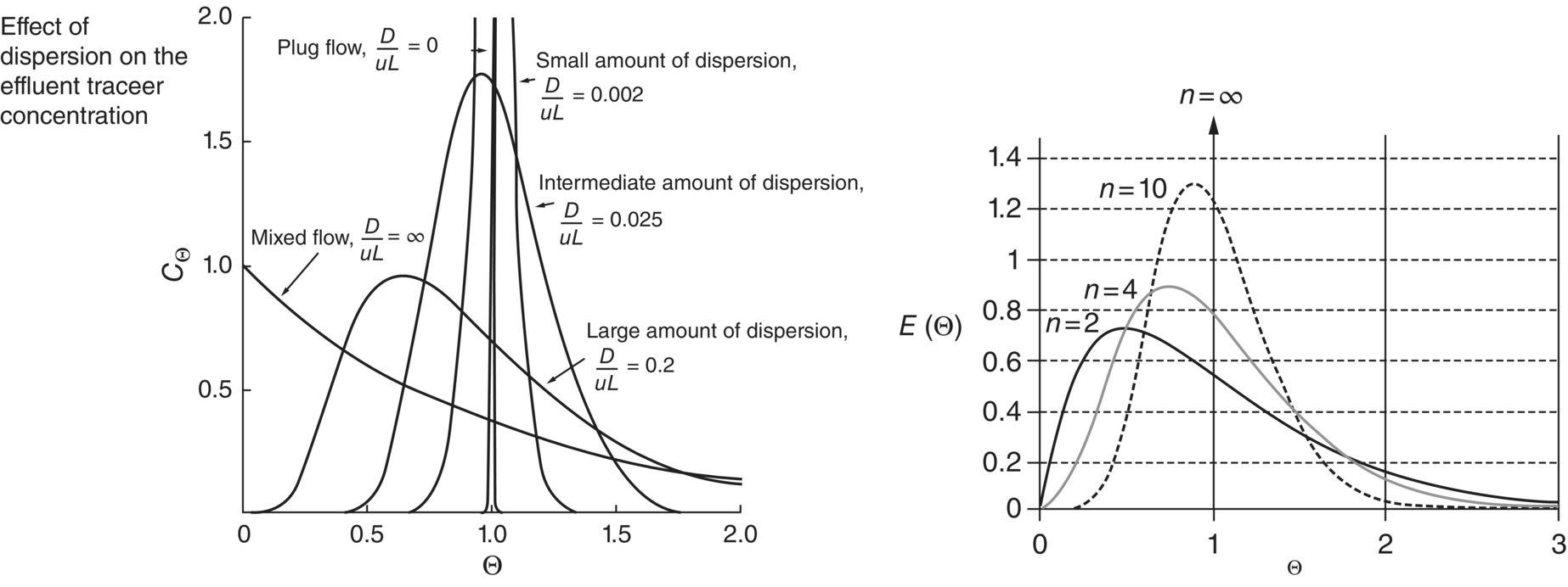
FIGURE 15.8 Effect of the concentration of a pulse based on the axial dispersion into a reactor.
Source: From Fogler [29]. Reproduced with permission of John Wiley & Sons.
The RTD of reactors can be used in association to kinetic models to evaluate the performance of a process during state of control and when disturbances occur. In addition, RTD is often used during the execution of the control strategy for traceability of materials.
Over the years, several methods have been developed to measure the micromixing time. Among them, two are well established, Bourne IV and Villermaux–Dushman [30, 31]. Villermaux–Dushman can be seen as the method of choice as it provides a protocol associated with the mean (IEM) mixing model to quantify the micromixing time based on the selectivity between two reactions, an estimated instantaneous reaction and a really fast reaction with their rates constant well defined. The concentration ratio between the two products could directly be linked with the mixing time of the equipment and the mixer (Figure 15.9).

FIGURE 15.9 Table of characterized meso‐reactors and mixers using the Villermaux–Dushman protocol and IEM model.
15.3.5 Process Simulation
Statistical models such as design of experiments are commonly used in the pharmaceutical industry: first, during process development to support process knowledge by mapping out yield and quality of the product as a function of process parameters input and then, during the registration of the DS and the DP to demonstrate the control of the process during manufacture. More recently, supported by the regulatory agencies, the pharmaceutical industry has been seeking not only for process knowledge but also for process understanding to feed into the quality by design (QbD) approach. Originally developed for the oil and gas and the bulk chemical industry, various commercial simulation companies have adjusted their products to be more aligned with the pharmaceutical industry requirement and to respond to the change of strategy. Continuous processing in the pharmaceutical industry covers reaction and workup; however, the most significant part remains chemical transformations. Therefore, emphasis was made to the kinetic aspect of the model to respond to the complexity of the transformations. In addition to the kinetic and thermodynamic expressions, the physical rates of heat and mass transfer were added to allow prediction of complex nonuniform behaviors. As described in Section 15.3.4, following the characterization of the equipment, heat transfer, mixing rate, and axial dispersion can be added to a kinetic model. The development and industrialization of continuous processes for pharmaceutical application is a difficult task due to the intrinsic interaction between the process rates, of often fast and complex reactions, and the physical rates associated with the equipment. These models play a key role in a successful continuous process development and implementation into manufacturing facilities.
15.3.5.1 Process Optimization and Design Space Definition
Following the definition of the model, including the verified kinetic and thermodynamic expressions of the process and the relevant expression of the physical rates of heat and mass balance, the model can be used to execute a comprehensive optimization of the process. A list of process parameters must be selected with initial guessed values and boundaries. Usually, the boundaries are the one used for the verification of the model. Then, an objective function must be defined, which is usually relative to yield, process performance, and product quality. However, process robustness and process CoGs can be defined as objectives too. The objective function is usually defined either against a set target, for example, a yield greater than 95% w/w and impurities lower than 0.1% w/w or against a maximize/minimize function, for example, minimize impurity level and CoGs. To achieve the optimization, a large list of algorithms is available; the most commonly used are simplex linear algorithms [32] or least square methods [33].
Simplex algorithm, for linear programing, is operating by defining a vector in a geometrical figure. It proceeds by performing successive pivot operations, the least optimal point is discarded, and a new vector is defined. It usually operates by following one of the four following actions: reflection, reflection with expansion, contraction, and multiple contractions.
The least square method minimizes the squared residuals between the data generated and the fitted values provided by a model for every single equation. It exists as linear and nonlinear. For the linear least square method, the model includes a linear combination of the parameters, and it has a closed‐form solution. For the nonlinear method, the problem is solved by iterative refinement. At each iteration, the system is approximated by a linear solution. It is important to notice that in the linear least square method, the solution is unique. However, in the nonlinear least square method, there may be multiple minima in the sum of squares (SSQ).
Process optimization is not limited to the definition of the operating set point where the optimum function is converging to a global minimum. Process optimization can equally include the definition of the design space capturing ranges of conditions where the objective function is still valid. This design space represents the boundaries where the process fails or passes the specification defined. In addition, depending on the definition of the objective function, the process design space can include risk and robustness of the process for manufacture.
15.3.5.2 Reactor Definition and Selection
The process development phase supported by a deep process understanding of the kinetic and thermodynamic processes can be linked to the identification of manufacturing technology. Ground rules are applicable for the selection of the equipment; however, process simulation with the opportunity to solve complex problem becomes an efficient design and selection tool. Sensitivity studies of the process output against the process parameters can be performed. The impact of each process parameter can be analyzed independently or globally within verified range of the model. Process simulation allows a more complex sensitivity analysis coupling multiple process parameters together.
From this in silico exercise, the impact of the input parameters to the process can be predicted. The required range of physical rates of heat and mass transfers are calculated to achieve the yield, quality, CoGs, and robustness predefined for the process. The information generated with the support of the process model can be incorporated in a reactor user requirement specification (URS) or reactor datasheet to be shared with equipment suppliers. The purpose of this exercise is to identify the optimum technology to run the process. From the nature of the chemistry studied, flow equipment is most likely to be selected. However, in some cases, batch or semi‐batch type of process still provides the desired yield and quality output with the addition of flexibility. Using process simulation as schematized in Figure 15.10 allows to only consider the process benefits.
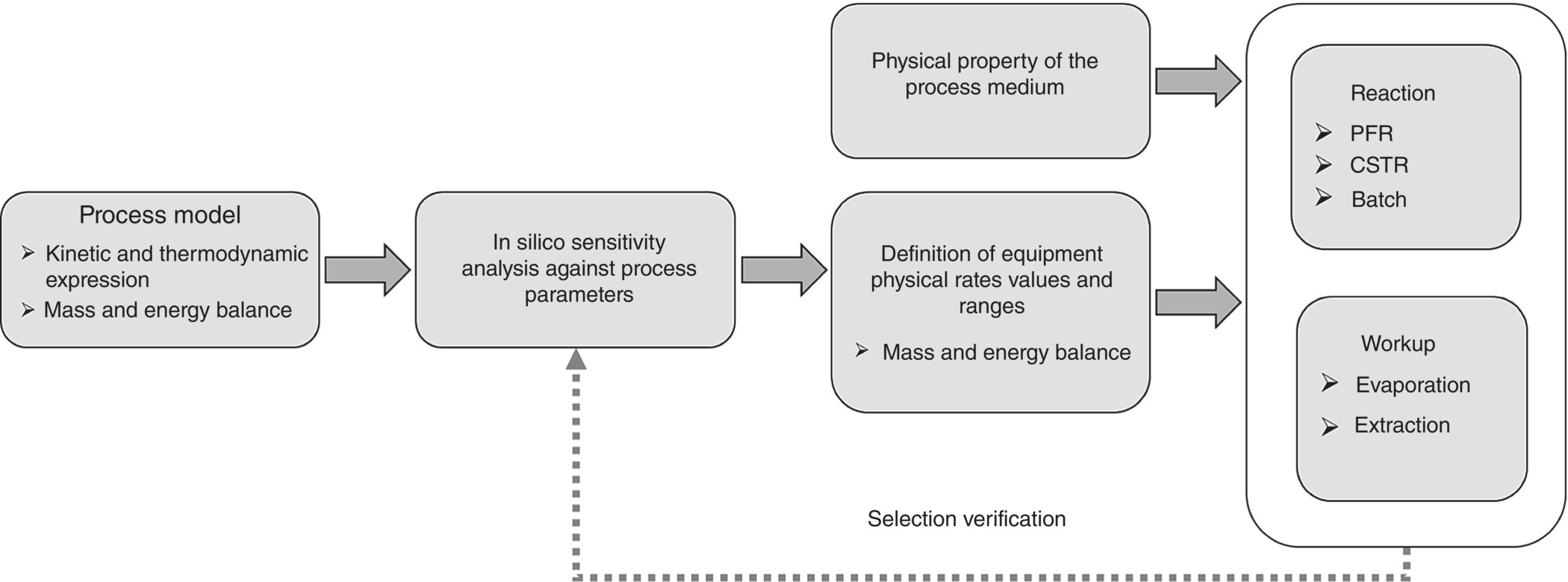
FIGURE 15.10 Workflow for equipment selection using process modeling and sensitivity analysis.
15.4 CONTINUOUS TECHNOLOGY
Continuous operation in the pharmaceutical industry is often focusing on reaction as the value is mostly seen in the chemical transformation rather than in the process and unit operation enhancement. However, continuous technology covers a wide array of unit operations demonstrating benefit across reaction, workup, and isolation. Tubular reactor, continuous extraction, and continuous evaporation technologies are now making their way from other industry into the pharmaceutical industries. However, to fully respond to the process complexity and the low volume requirement, additional technologies have emerged from university spin‐off and small and medium enterprises (SMEs). Pharmaceutical continuous technology is the combination of the well‐established and the new state‐of‐the‐art technologies.
15.4.1 Chemical Reactors
15.4.1.1 Plug Flow Reactors and Static Mixers
PFRs are the most common type of reactors used in pharmaceutical industry as a replacement of batch technology. The equivalence of batch reaction time is residence time under ideal plug flow conditions simplifying their implementation. Their enhanced performance in heat and mass transfer is the perfect response of the initial intent, enabling fast and temperature‐sensitive chemical transformations. PFR is a versatile technology; as demonstrated across various applications in the oil and gas and the polymer industries, when operating at high flow velocity and high Reynolds numbers, they are efficient in adding or removing heat to a process stream due to their high heat transfer coefficient and surface to volume ratio. They are very efficient in mixing miscible fluid streams quickly and homogeneously in a compact volume both for laminar or turbulent flow regimes and for streams with similar or widely different viscosities. To maximize the performance of PFRs, tubular reactors often integrate static mixers.10–13 Multiple types of insert are currently available from high to low mixing capacity (Figure 15.11).
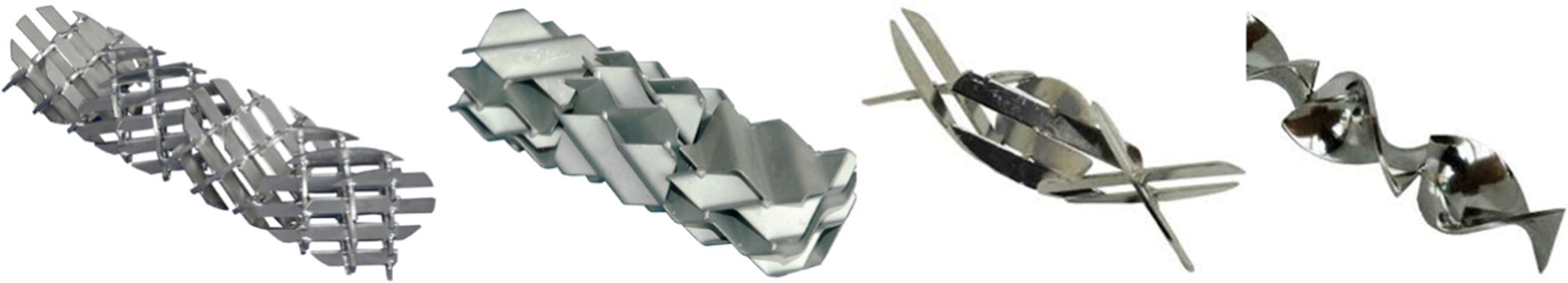
FIGURE 15.11 Static mixers used to enhance heat and mass transfer of tubular reactors. From left to right, arranged by efficiency, high density grid, corrugated, low density grid, and helical static mixers.
Source: Courtesy of Sulzer.
Such inserts can be added on the shell and process media side as they minimize the impact of the contribution of the inner film (hin) and outer film (hout) to the overall heat transfer by enhancing the velocity by the wall. In addition to the effect on heat transfer, static mixers are generally used to enhance the mass transfer performance of tubular reactors. Quick micromixing time or blending time is usually achieved by using dense elements with high pressure drop associated. The efficiency often relies on the capacity to slip and recombine layers of the process stream until full homogenization of the process flow is achieved (Figure 15.12).
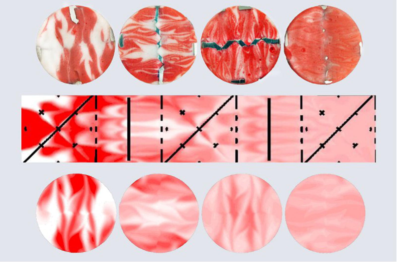
FIGURE 15.12 Cross section of an intensive high density grid static mixer during mixing of two streams.
Source: Courtesy of Fluitec.
In addition, static mixers have the effect to minimize the RTD in the reactor, with Bodenstein numbers of up to three L/D (L and D being length and diameter of the reactor tube, respectively).
Static mixer can also be used for multiphase systems to generate droplets of one immiscible liquid stream into another or gas bubble in a liquid stream (Figure 15.13). In this case, the mixers are usually operated in the mist flow regime, where films form on the surfaces of the static mixer and at the same time droplets are present in the gas flow. Such installations are often used to enhance mass transfer of a dispersed liquid or gas in a liquid stream. Such biphasic application could equally be used for cleaning procedure, scrubbing residuals out of an equipment, or for the evaporation of a liquid in a hot gas stream.

FIGURE 15.13 Generation of droplet in high intensity grid static mixer.
Source: Courtesy of Sulzer.
15.4.1.2 Plate Reactors and Meso Channels Reactors
The enhancement of heat transfer has been achieved in flow processing by the significant increase of surface to volume ratio of the reactors. As described in Section 15.4.1.1, PFR can provide significantly greater heat transfer coefficient than standard batch vessels. However, alternative designs to standard PFRs can even further improve the heat transfer. Among these designs, we can find plate or meso channel reactors (Figure 15.14). Their surface to volume ratio can be increased by two orders of magnitude, resulting in examples where U > 3000 W/m2∙K. can be achieved. In addition, their small ID maximizes the efficiency of micromixing by enabling a high flow velocity.
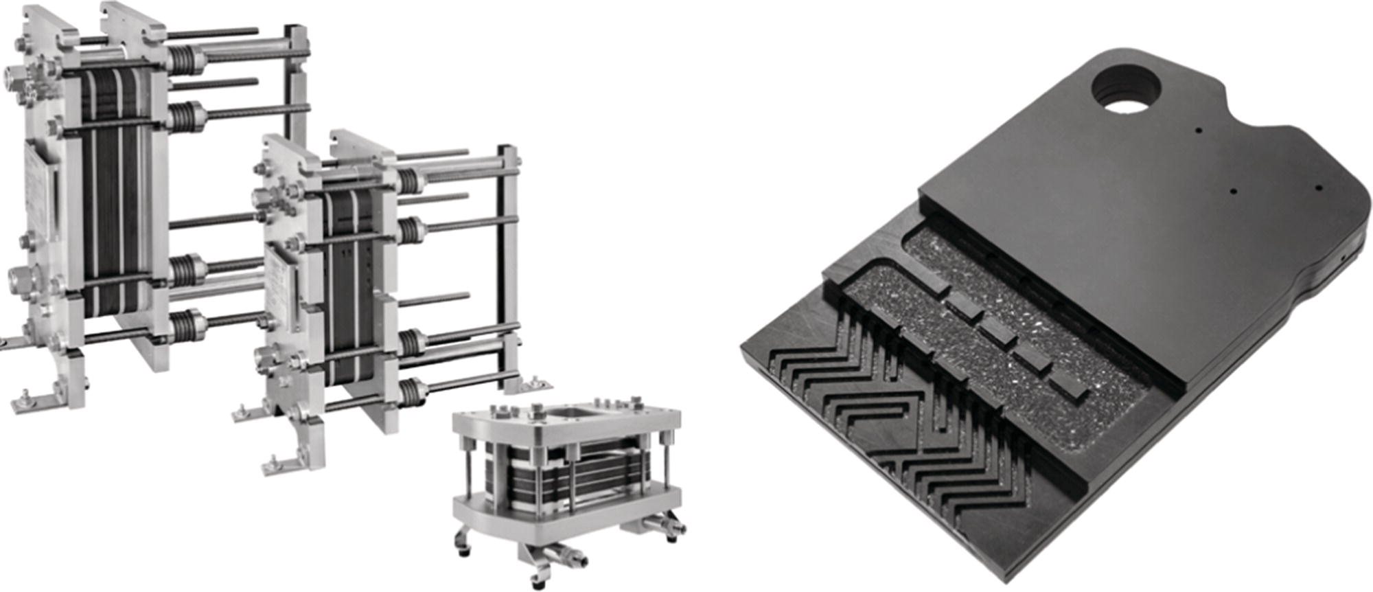
FIGURE 15.14 Schematic of plate reactor design and assembly of multiple elements.
Source: Courtesy of Chemtrix catalog.
However, the design of these reactors provides some limitations to their use. Due to the small channel cross sections, the pressure drop reaches a high value even at low flow rate, lowering their potential productivity rate. In addition, their capability of handling solid remains limited and the reactor becomes subject to fouling.
Tubular and plate reactors have been, so far, the preferred technology of the pharmaceutical industry, as the high plug flow behaviors minimize the axial dispersion and allow a tight control of the genealogy of the product, minimizing the risk of product loss associated with deviations and contaminations.
15.4.1.3 Continuous Stirred Tank Reactors
Continuous stirred tank reactors (CSTRs) are often underutilized in the pharmaceutical industry to the favor of shell and tube reactors and high plug flow behavior reactors. However, the simplicity and versatility of these reactors make them extremely attractive to continuous operation. Their design is similar to standard batch reactors with a height to diameter ratio (L/D) around 1 and an elliptical bottom. The flow through the reactor is provided by constant feed using pumping or pressure, and the flow out is enabled by controlled pumping or valve systems connected to level controllers or in some cases by a simple gravity connection.
The mixing is provided by the mechanical agitation of an impeller, and the heat transfer is delivered by standard outer wall jacket. CSTRs rarely exceed a heat transfer coefficient of 300–400 W/m2∙K and their macromixing time is often, depending on size and design, at least one order of magnitude lower than the blending time achieved between miscible streams in PFRs at high flow velocity. Despite these obvious limitations, CSTRs provide some specific advantages. First, as the mixing is decoupled to the flow velocity, good mixing efficiency can be achieved at even low flow rate. This mixing efficiency can be even further enhanced by the implementation of the baffle system, by tailoring the impeller type to the physical property14 (Figure 15.15) or by the implementation of jet mixing through recirculation.
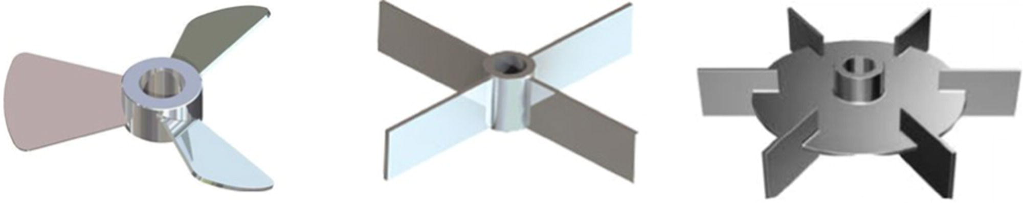
FIGURE 15.15 Type of impellers providing different mixing properties and flow directions from single to multiphase processes and different viscosities.
Source: KMPS.
In contrary to most of the overflow technology, CSTRs have the ability to handle solids up to 10–15 w/w mass fraction. As chemical transformations in the pharmaceutical industry often contain solid base reagents or precipitate (product or by‐product), CSTRs offer an alternative enabling continuous operation where other technology cannot be applied.
CSTRs can be operated as high dilution system. Therefore, the concentration profile achieved at state of control is significantly different to PFRs. This could offer a significant advantage to the control of side product formations and second‐order decomposition of starting materials.
15.4.1.4 Packed Bed and Trickle Bed Reactors
Continuous packed bed and trickle bed reactors have been the expertise of the bulk chemical and petrochemical industry for decades. In these industries, the implementation of such technology targeted improvement of the process efficiency, resulting to substantial reduction of process cost. Currently, pharmaceutical portfolio analysis reveals that up to 20% of the chemical transformation to the DS contain catalytic gas/liquid transformations. Therefore, pharmaceutical companies are now devoting significant efforts, shifting traditional batch solid–gas–liquid operation to flow processes. Packed bed and trickle bed reactors are the key technology to unleash these cost benefits. Through decades of development, the oil and gas industry generated a significant amount of knowledge for the development of three‐phase reactions, in particular, the hydrosulfurization or hydrocracking of heavy oils and the hydrotreating of lubricating oils. However, the tonnage of pharmaceutical processes is significantly lower, and the variety of transformation on which three‐phase reactions are applied is knowingly more complex and subject of significant number of by‐product formations. For these reasons, not only a transfer of the knowledge is required, but also new sized equipment associated with new type of catalysts must be developed. For existing suspended catalytic transformations in batch reactor, over hundreds of different catalysts are referenced in catalogues from various suppliers to address the high requirement of selectivity of the pharmaceutical chemical transformations.
Despite the significant change required for the catalyst, the reactor fundamentally remains similar. This three‐phase reactor flows downward gas and liquid concurrently over a fixed bed of catalyst. Liquid trickles down, while gas phase is continuous. In a trickle bed reactor, various flow regimes can be observed, from trickle flow (low interaction) to pulse flow (high interaction), spray flow, and bubble flow regimes (Figure 15.16). The effect of bed geometry, flow velocity, and fluid phase properties are the key parameters impacting the reactor regime.
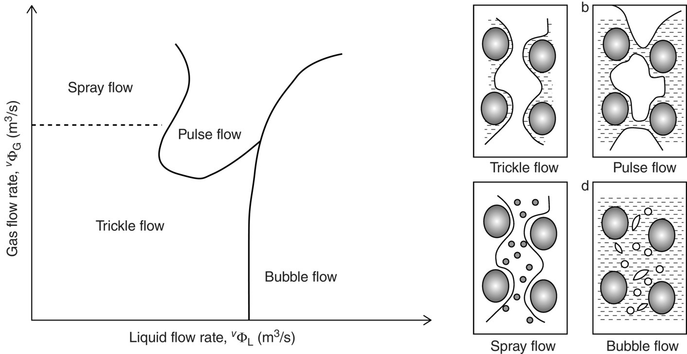
FIGURE 15.16 Schematic of the various flow regimes observed in trickle bed reactor due to the gas and liquid velocity.
Source: Reprinted from Nguyen et al. [34] Reproduced with permission of Elsevier.
Despite the multiple advantages demonstrated across processes in over industries, trickle bed reactors have complex fluid dynamic and therefore difficult to industrialize. Nonideal bed packing and nonuniform particle size distribution could lead to large deviation in flow behaviors, and bypassing and inefficient contacting can be observed. Despite the low shear applied by the flow, catalytic bed can be eroded, leading toward degradation of the bed behaviors and change of pressure drop in the system over time. Therefore, to enable efficient operation, the analysis and design of the multiphase reactor become a critical part of the process development. It is recommended to follow a three‐phase strategy [35] for the selection of the type of multiphase reactor. The first level focuses on the catalyst design such as activity, shape, particle size distribution, and strength. The second level is about the phase injection and dispersion onto the catalytic bed. The final level is the understanding of the hydrodynamic of the multiphase flowing onto the bed.
15.4.1.5 Extraction Columns with Trays and Packings
Static extraction units are generally used for simple extraction applications that do not have significant change in the volumetric flow rate for the carrier feed stream and where there is little change in the fluid densities, viscosities, and interfacial surface tension. Several static extractors are available with different relative capacities and efficiencies. Spray columns are the simplest and oldest extractors. Dispersed‐phase droplets simply rise (or fall) through the continuous phase in an empty column. Therefore, these units are susceptible to axial mixing, which generally prevents them from achieving more than one nominal theoretical stage of separation.
Structured or random packing can be added to spray columns to reduce axial mixing. Movement of the droplets across the packing surfaces induces turbulence inside and outside of the droplets, which accelerates the mass transfer. Structured packing surface is perforated and usually supplied with smooth surface. The periphery of the packing elements is equipped with a specialized wiper band to reduce wall effects. The corrugated sheets of the packing element guide the direction of flow within each layer. Some aspects of the structured packing material and wetting by the extraction fluids need to be considered. In general, the metal packing surface is wetted by the aqueous continuous phase, and plastic packings are wetted by the organic continuous phase. The dispersed droplets coalesce together when they reach the next sieve tray deck, and droplets form as the dispersed phase flows through the holes.
Pulsation can be added to static extraction units to enhance mass transfer. Such columns are equipped with static internals like structured packing or dual‐flow sieve trays. Bellows or a pulsation pump provides oscillating pulses to the continuous phase. This improves the mass transfer efficiency but reduces the hydrodynamic capacity of the column. The main drawbacks of pulsation are high costs and energy consumption.
15.4.1.6 Agitated Extraction Columns
In the range of extraction columns with energy input, two main principles apply, pulsation and agitation. An overview about agitated extraction columns can be found in various engineering books [36–38]. The basics of this technology are still the same as in the rotating disc contactor (RDC). The column is vertically divided into compartments, and each compartment has a mixing element mounted on a common shaft. The mixing element was improved starting from the simple disc in a RDC to paddle and turbine agitators as applied in the Scheibel and Kuhni as shown in Figure 15.17. The aim of all developments is to improve the separation performance of the column and increase the throughput. Mainly this is achieved by improving the agitation in the column compartments to intensify the phase contact and to reduce the axial back mixing with optimized partition plates between the individual compartments.

FIGURE 15.17 Examples of different types of extraction column and their efficiencies.
Source: Courtesy of KMPS.
The main benefit of the agitated columns is the wider flexibility and high separation performance as shown by Kumar and Hartland [16] compared with other column technologies. The agitated column type ECR covers the entire operating of RDC, simple spray columns, and pulsed sieve plate columns while providing a significant higher separation performance at high throughput. These columns are also well known for adapting the internals to cope with high mass transfer and changing physical properties over the column height.
15.4.1.7 Annular Centrifugal Extractors
An alternative to gravity separation is centrifugal extractor (Figure 15.18). The technology was initially used to enhance the separation of hydrocarbon and water, solvent recovery, and waste treatment in the nuclear industry. Compared with the gravity separator, centrifugal extractors have a really short contacting time and residence time preventing degradation.
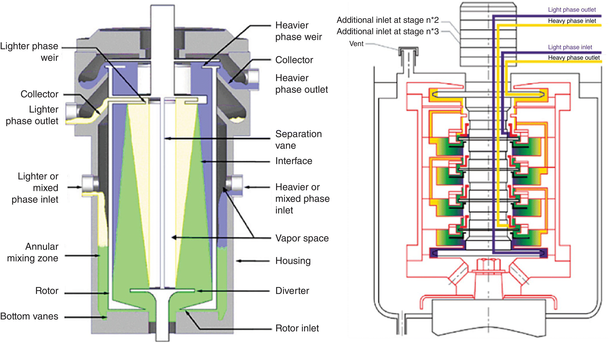
FIGURE 15.18 Single and multistage centrifugal extractor with design and flow routes.
Source: Courtesy of Rousselet Robatel.
The two immiscible liquids are fed to the extractor and are rapidly mixed in the annular space between the spinning rotor and stationary housing. The mixed phases are directed toward the center of the rotor by radial vanes in the housing base. As the liquids enter the central opening of the rotor, the mixed phases are rapidly accelerated to rotor speed and separated based on their density difference. Annular centrifugal contactors are relatively low revolutions‐per‐minute (rpm), moderate‐gravity‐enhancing (100–2000 G) machines and can therefore be powered by a direct drive, variable speed motor. The effectiveness of a centrifugal separation can be easily described as proportional to the product of the force exerted in multiples of gravity (g) and the residence time in seconds or g‐seconds. Achieving a particular g‐seconds value in a liquid–liquid centrifuge can be obtained in two ways: increasing the multiples of gravity or increasing the residence time.
This technology has seen its number increasing in pharmaceutical industry as it provides a solution for implementation of continuous extraction with a linear and easy path from laboratory to large‐scale facilities.
15.5 PROCESS DESIGN METHODOLOGY FOR ORGANOMETALLIC CHEMISTRY IN CONTINUOUS: FROM R&D TO MANUFACTURE
15.5.1 Introduction
Organometallic reagents, such as Grignard’s and organolithium compounds, are frequently used within the pharmaceutical industry. Process design associated with organometallic chemistry is often governed by traditional batch controls of low temperatures and long hold durations to accommodate the poor heat transfer and limit process degradation [39]. Process development and industrialization of challenging organometallic chemistries in flow is greatly relevant as it is part of a large number of pharmaceutical assets.
This case study summarizes the process methodology described in the sections above to continuous process development of the synthesis of 3‐borono‐5‐fluoro‐4‐methylbenzoic acid (compound A; Figure 15.19), a proposed registered starting material for the synthesis of Losmapimod, a p38 kinase candidate.

FIGURE 15.19 Proposed starting material (A) in the formation of Losmapimod.
The design approach focuses on fundamental mechanistic understanding and kinetics of main reactions and degradation pathways. Combined with calorimetric data, this allows the mass and energy balance of the process to be simulated in silico.
Compound A had initially been prepared from 3‐fluoro‐5‐iodo‐4‐methylbenzoic acid (compound B; Figure 15.20) by protection as the methyl ester, conversion to the Grignard reagent, quenching with triisopropyl borate followed finally by hydrolysis of the methyl ester. A transformation directly from the carboxylic acid B, with in situ protection by deprotonation, had been proposed following the work of P. Knochel [40, 41].
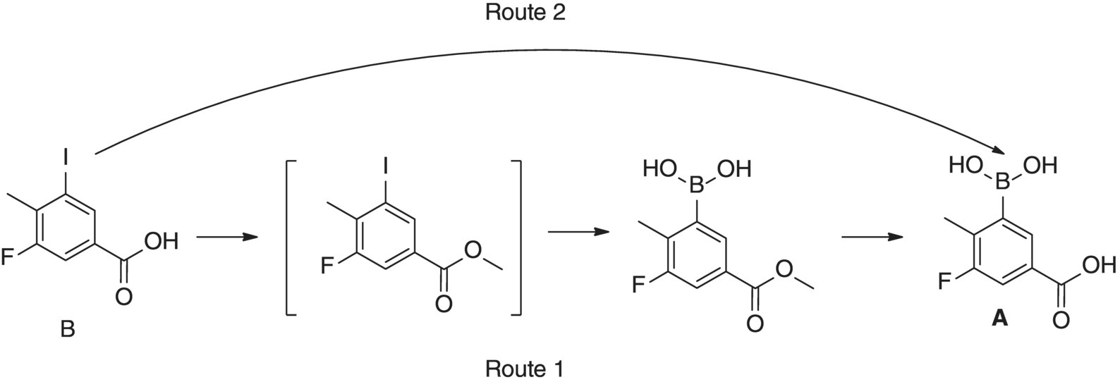
FIGURE 15.20 Proposed alternative synthesis of A to prevent protection and deprotection.
It was shown that methyl magnesium chloride showed good selectivity for deprotonation of compound B over halogen–magnesium exchange. Excess methyl magnesium chloride does undergo the exchange reaction to generate the desired aryl Grignard (compound D). Unfortunately the methyl iodide side product was found to quench the intermediate generating 3‐fluoro‐4,5‐dimethylbenzoic acid (compound F). This degradation reaction of the aryl Grignard was not observed when isopropyl magnesium chloride was used for the exchange reaction, giving 2‐iodo‐propane as the side product. Therefore, a sequential deprotonation with methyl magnesium chloride then halogen magnesium exchange with isopropyl magnesium chloride was required to generate Grignard reagent D, which could be quenched with trimethyl borate (introduced for improved atom efficiency) giving compound A after hydrolytic workup. The intermediates are unstable and moisture sensitive and decompose over time with strong temperature dependence. This sequential process is dependent on precise reagent charges and efficient mixing, making it an ideal candidate for flow operation. The intent was to enable tight control of the critical process parameters by utilizing flow chemistry to the organometallic transformation. The borate quench, aqueous workup, and final isolation were completed as batch operations.
15.5.1.1 Methodology of Development
To enhance process understanding, a detailed study of the reactions was undertaken. The objectives of the study was to measure reaction calorimetry, estimate kinetic parameters for both the main process reactions, deprotonation and exchange, and degradation pathways as indicated in Figure 15.21 and to understand the impact of physical rate effects to yield and quality. Experimentation was completed in the most appropriate technology as discussed below. The equipment selected for the study were fully characterized (mass and heat transfer) to ensure accurate interpretation of the data.

FIGURE 15.21 Deprotonation metalation borylation and hydrolysis to compound A and postulated decomposition pathways.
To generate the reaction process understanding, two systems were used in response of the dynamic of the various reactions. The degradation kinetics, being slow enough, were monitored using small automated batch reactors15 to evaluate impurity formation against process parameters and time. The main reactions were studied at steady state using a bespoke flow system as indicated in Figure 15.22. The substrate and the reagent were delivered and controlled using a HNP microannular gear pump16, SyrDos syringe pump,17 and Bronkhorst Coriolis mass flow meter18 at ambient temperature. The streams were brought together using two different characterized passive mixing devices; Ehrfeld HC10 Cascade mixer19 and standard 1/16″ Swagelok tee piece were used to evaluate the impact of mixing. The output mixture was then passed through variable lengths of polytetrafluoroethylene (PTFE) pipe with an internal diameter of 1/32″. Length of the pipe was used to adjust system residence time to 0.4, 0.3, 0.2, and 0.14 second. The mixture was then analyzed in‐line using a Mettler Toledo flow IR20, and additional samples were collected for off‐line HPLC analysis.
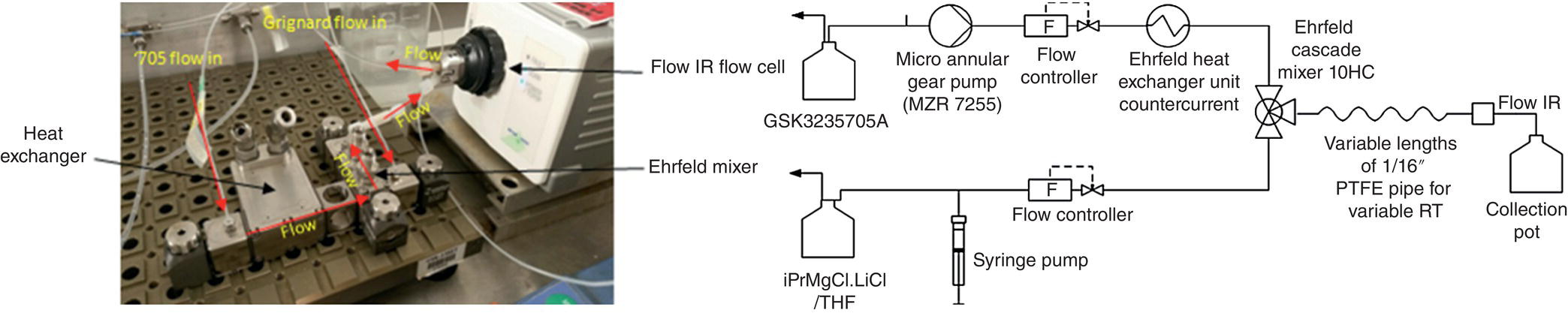
FIGURE 15.22 Photograph of fast kinetics rig and equipment line diagram for fast kinetics rig.
To keep the methane generated during the deprotonation in solution, the pressure in the system was controlled with a back pressure Equilibar membrane device at 7 bar. This value was calculated using Henry coefficient for pure solvent with an extra precautionary allowance factored in to compensate for nonideal behaviors.
15.5.1.2 Kinetic Model
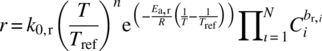
A kinetic model was developed using both DynoChem and MatLab to describe the main transformations and side reactions described in Figure 15.21. All reactions were modeled as second‐order reactions; therefore, the rate equation can be expressed as shown in Eq. (15.18) where the rate constant, k, is expressed in terms of the activation energy (EA) by the Arrhenius equation:
Time course profiles were generated for the degradation of intermediate C and D at various temperature and concentration as shown in Table 15.1.
TABLE 15.1 Description of Experiences Used to Generate the Process Understanding and Regressing the Kinetic Parameters
| Reaction | SM Concentration (M) | MeI Concentration (M) | MeMgCl Concentration (M) | Temperature (°C) |
| 1 | 0.15 | 0.165 | 0.195 | 30 |
| 2 | 0.15 | 0.165 | 0.195 | 30 |
| 3 | 0.15 | 0.165 | 0.195 | 30 |
| 4 | 0.15 | 0.165 | 0.195 | 40 |
| 5 | 0.15 | 0.165 | 0.195 | 50 |
| 6 | 0.15 | 0.135 | 0.195 | 50 |
| 7 | 0.15 | 0.225 | 0.195 | 50 |
| 8 | 0.15 | 0.165 | 0.1575 | 50 |
| 9 | 0.15 | 0.165 | 0.1575 | 20 |
| 10 | 0.15 | 0.165 | 0.225 | 50 |
| 11 | 0.15 | 0.165 | 0.225 | 20 |
Those batch kinetic data generated for the degradation of the intermediates were used, in a standard batch mechanistic model, where the mechanism described in Figure 15.21 was converted into differential rate equations. The activation energies and rate constants were regressed as shown in Figure 15.23 by using the weighted total SSQ of the deviations between the data and model results to ensure an accurate fitting of the various profiles regardless of the respective contribution to the mass balance and the number of points.

FIGURE 15.23 Examples of mol % versus time profiles for degradation of compound C (left) and compound D (right) generated at various temperatures and concentrations.
The estimation of the kinetic parameters achieved using the Levenberg–Marquardt algorithm and the weighted SSQ as objective function were reported in Table 15.2.
TABLE 15.2 Kinetic Parameters for Each Transformation Considered as Relevant to the Process
| KTref | EA | |||
| Main Reaction | ||||
| B + MeMgCl → C + Methane | 1 × 10² min−1 | (Observed) | 60 kg/mol | (Observed) |
| C + iPrMgCl → D + iPrI | 1 × 10² min−1 | (Observed) | 60 kg/mol | (Observed) |
| Degradation | ||||
| C + MeMgCl → D + MeI | 0.03 min−1 | 39 kg/mol | ||
| C + MeMgCl → Degradent | 4 × 10⁻³ min−1 | 54.4 kg/mol | ||
| D + MeI → F + MgClI | 0.03 min−1 | 45 kg/mol | ||
Due to extremely fast reaction and significant exotherm (ΔHr = −220 kJ/mol, ΔTadd = 77 °C for the deprotonation reaction, ΔHr = −210 kJ/mol, ΔTadd = 64 °C for the exchange reaction), generating valuable kinetic data for the main process reaction was achieved with great difficulty, and non‐isothermal conditions were observed with a significant dependence to mixing. To address the interdependence between the kinetic and the physical rates, the performance of each part of the set up was characterized. The heat transfer and area (UA) was calculated through heat loss measurement experiments; the micro‐mixing time was calculated as a function of flow rates using the Villermaux–Dushman procedure, and the axial dispersion was estimated using standard mathematical expression for the Bodenstein number as described in Section 15.3.3.
The flow steady‐state system used for generating kinetic data resulted in conclusion that the desired reaction steps were complete in less than 140 ms, faster than it was possible to quantify using the setup. This was the case across a range of dilutions and temperatures. Based on this knowledge, observed rate constants and activation energies were applied, which satisfied these conditions (Table 15.2).
The partial differential equations for each transformations and side reactions were integrated into a series of PFR models in both DynoChem and MatLab to be the exact in silico representation of the existing setup described in Figure 15.21. In addition to the mechanistic description, the physical rates calculated and specific to the capillary PFR were included into the model.
15.5.2 Process Design
Some documented studies of transformations of organic molecules using Grignard reagents at room temperature are recorded in the literature, ranging from the micro‐ to mesoscale [42–44] with reduced or no heat transfer; however little supported understanding of the process kinetics is documented. This kinetic understanding is crucial for process scale‐up where different temperature profiles due to change of heat transfer and heat loss reduced mixing efficiencies and more challenging control of residence times.
The PFR model including a full kinetic description of the process with the physical rates associated as described in the section above allows the evaluation of the process parameters and their impact to the product quality output. Impact of temperature was investigated in silico by enabling various heat transfer performance of the reactor from high heat transfer coefficient to adiabatic conditions. Impact of mixing time and nonuniformity of the concentration gradient across the length of the reactor was assessed from instantaneous to slow mixing. Impact of axial dispersion was equally studied from ideal plug flow to high axial distribution and small reactor equivalence.
Following a global sensitivity analysis, it demonstrated that axial dispersion and micromixing did not have limited impact as long as the mixing time was faster than the residence time and the equivalence of reactors was greater than 5 units. Equally, up to 0.5 second residence time and adiabatic conditions could be tolerated with acceptable impact on the product quality. It negates the need to reduce the system to cryogenic temperatures and simplifies the process control requirement and the reactor design.
15.5.3 Equipment Design
After completion of the process design, the various performance attributes of the reactor, enabling high yield and high quality, were captured in a user specific requirement document to support the design and construction of the equipment. Working alongside technology specialist, the design of the tubular reactor, injector, and static mixer was completed (Figure 15.24).
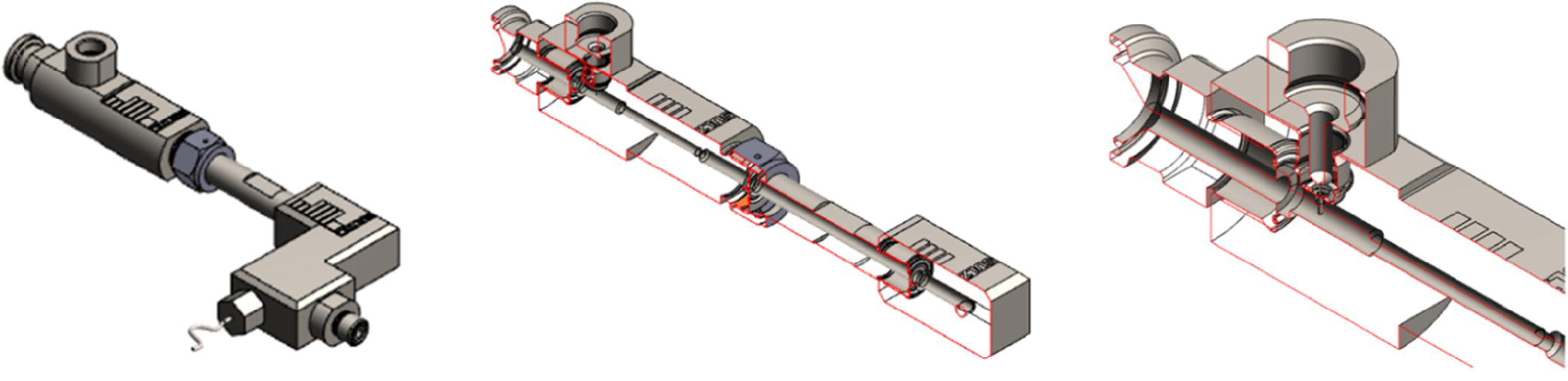
FIGURE 15.24 3D drawing of the reactor design.
Specific attention was brought into the design of the injector to ensure robustness during operation as solid was observed. The injection system was designed to prevent back mixing and local concentration excess of organometallic. The side stream was injected at the point of highest turbulence to ensure the most efficient blending of both streams into each other. In addition, the design of the static mixer was reviewed with the supplier to ensure maximum efficiency for this process, and SMX‐plus static mixers21 were selected. The main inner body of the reactor was 4.8 mm diameter as the injector was 0.3 mm. The overall length of the reactor was only 300 mm before reaching an elbow connector where a thermocouple type K was inserted to measure the temperature of operation with an accuracy of ±0.5 °C. The same exact design was used for both transformations.
Following the construction of the reactor, a series of tests, as part of the site acceptance test (SAT), were completed to ensure the performance of the unit against the initial requirements. RTD, micromixing time, and heat loss were measured through a series of experiments (Figure 15.25).
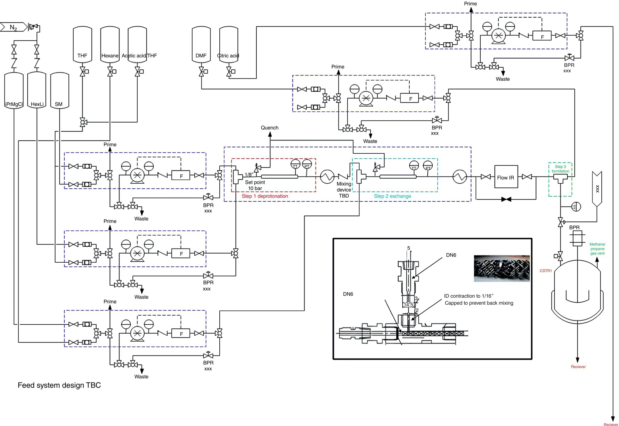
FIGURE 15.25 Process and instrumentation diagram for the two‐stage flow process.
Using the in‐process model including the kinetic of the desired reaction, the side reactions, and the equipment performance, the optimum conditions were identified as described on the contour plots below (Figure 15.26).
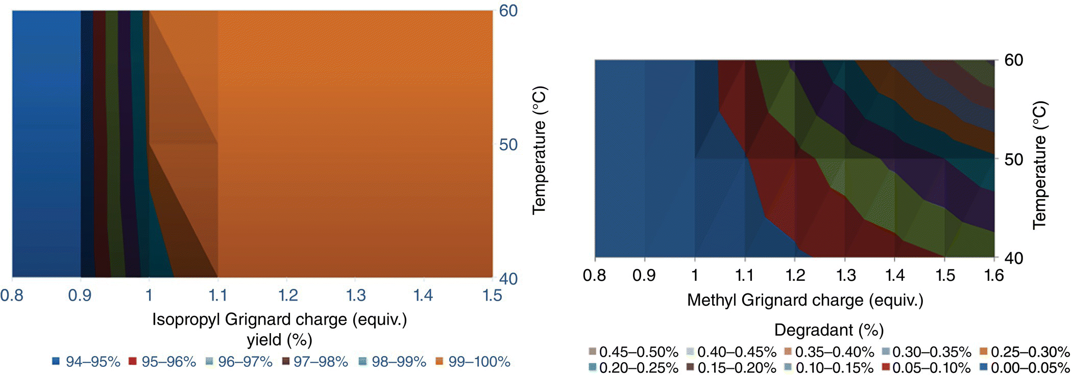
FIGURE 15.26 In silico representation of yield and overall degradants as a function of process conditions.
The resulting operating conditions are described below.
A solution of compound B in tetrahydrofuran (THF) (4.4 wt %, 0.14 M) was combined with methyl magnesium chloride (3 M, 22% w/w 1.15 equiv.) in a PFR matching all the above performance characteristics (Bodenstein number, mixing time, and heat loss) for a residence time of 0.50 seconds. The resulting solution was then combined with isopropyl magnesium chloride (2 M, 20% w/w 1.1 equiv.) using similar PFR for an additional 0.50 second residence time. The aryl Grignard solution was then cooled to −15 °C and quenched by addition of trimethyl borate (2.5 equiv.) in a batch reactor. The resultant component E solution was worked up by adding 2 vol of 15% w/w sodium chloride aqueous solution and a 50% w/w aqueous citric acid (4 vol, 3.6 equiv.) followed by phase separation. The organic phase was then washed three times with sodium hydroxide (4 M, 5 vol), and the basic aqueous streams are combined. The combined aqueous base stream is then overlaid with cyclopentyl methyl ether (CPME) (6 vol) and then acidified by the addition of hydrochloric acid. The organic phase containing component A is washed with brine (26% w/w), concentrated to 6 vol (0.6 M) by vacuum distillation, and then the product is precipitated by the addition of 2,2,4‐trimethylpentane (10 vol). The slurry is then filtered, and the solid is washed with CPME:2,2,4‐trimethylpentane (3 vol).
Prior to the clinical campaign, the process was successfully verified in a kilogram continuous demonstration. Several batches of 1 kg of compound B were processed, collected, and isolated in 500 g batch of compound A yielding 70% as described in Table 15.3.
TABLE 15.3 Experimental verification of the process design
| Reaction | SM Flow Rate (g/min) | MeMgCl Flow Rate (g/min) | IsoPrMgCl Flow Rate (g/min) |
| 1 | 150 | 59 | 35 |
| 2 | 130 | 51 | 30 |
| 3 | 130 | 51 | 30 |
| 4 | 130 | 52 | 28.8 |
| 5 | 130 | 52 | 28.8 |
| 6 | 130 | 49 | 28.8 |
| 7 | 130 | 49 | 28.8 |
| 8 | 130 | 52 | 27.3 |
| 9 | 130 | 49 | 30.3 |
| 10 | 130 | 52 | 24.5 |
| 11 | 170 | 63 | 38.5 |
| 12 | 215 | 79 | 48 |
Following that demonstration, the process was transferred to pilot plant GMP facility to synthesize 200 kg of component B for a phase three clinical make.
15.5.4 Conclusion
A systematic approach using intrinsic process understanding and in silico enabled design has been shown to be an effective tool in the development of organometallic flow processes and industrialization. Low volume, residence time restricted systems allowed all processes to operate well outside of the usual cryogenic controls. By generating process understanding, such as quantification of kinetic constants and characterization of equipment, systems can be engineered to handle instable or hazardous chemistry while inherently increasing the process safety and sustainability.
The workflow employed successfully demonstrated the efficiency of integration of process simulation into the development and scale‐up of continuous processing. This offers significant advantages in terms of time and material saving, efficiency of scale‐up, and process robustness. Future application of this workflow could be used to reduce scale‐up risk, by formulating an in silico design space and verifying model predication across scales.
REFERENCES
- 1. Wiles, C. and Watts, P. (2012). Continuous flow reactors: a perspective. Green Chem. 14 (1): 38–54.
- 2. Malet‐Sanz, L. and Susanne, F. (2012). Continuous flow synthesis. A pharma perspective. J. Med. Chem. 55 (9): 4062–4098.
- 3. Strang, D. Pharma 2020: Supplying the Future. Which Path Will You Take? https://www.pwc.com/gx/en/pharma‐life‐sciences/pdf/pharma‐2020‐supplying‐the‐future.pdf (accessed 5 May 2017).
- 4. Abboud, L. and Hensley, S. (2003). Factory shift: new prescription for drug makers: update the plants. Wall Street Journal (3 September 2003).
- 5. IChemE (2004). Chemical Reaction Hazards – A Guide to Safety, 2e (ed. J. Barton and R. Rogers). Institution of Chemical Engineers.
- 6. Barton, K. and Rogers, R. (1997). Chemical Reaction Hazards. Elsevier.
- 7. Di Miceli Raimondi, N., Olivier Maget, N., Gabas, N. et al. (2015). Safety enhancement by transposition of the nitration of toluene from semi‐batch reactor to continuous intensified heat exchanger reactor. Chem. Eng. Res.Des. 94: 182–193.
- 8. Barton, J.A. and Nolan, P.F. Runaway reactions in batch reactors. I. CHEM. E. Symposium Series No. 85.
- 9. Willey, R.J. (ed.) Process Saf. Prog. 16 (2): 94–100.
- 10. Capellos, C. and Bielski, B.H.J. (1980). Kinetic Systems: Mathematical Description of Chemical Kinetics in Solution. R. E. Krieger Pub. Co.
- 11. Swarin, S.J. and Wims, A.M. (1976). A method for determining reaction kinetics by differential scanning calorimetry. Anal. Calorim. 4: 155.
- 12. Borchardt, H.J. and Daniels, F.J. (1956). The application of differential thermal analysis to the study of reaction kinetics. Am. Chem. Soc. 79: 41.
- 13. Ozawa, T.J. (1970). Kinetic analysis of derivative curves in thermal. Thermal Anal. 2: 301.
- 14. Mass, T.A.M.M. (1978). Optimalization of processing conditions for thermosetting polymers by determination of the degree of curing with a differential scanning calorimeter. Polym. Eng. Sci. 18: 29.
- 15. Hoffmann, W. (2007). Kinetic data by nonisothermal reaction calorimetry: a model‐assisted calorimetric evaluation. Org. Process Res. Dev. 11: 25–29.
- 16. Kumar, A. and Hartland, S. (1988). Mass transfer in a Kühni extraction column. Ind. Eng. Chem. Res. 27 (7): 1198–1203.
- 17. Keles, H., Susanne, F., Livingstone, H. et al. (2017). Development of a robust and reusable microreactor employing laser based mid‐IR chemical imaging for the automated quantification of reaction kinetics. Org. Process Res. Dev. 21 (11): 1761–1768.
- 18. Sarrazin, F., Salmon, J.‐B., Talaga, D., and Servant, L. (2008). Chemical reaction imaging within microfluidic devices using confocal Raman spectroscopy: the case of water and deuterium oxide as a model system. Anal. Chem. 80 (5): 1689–1695.
- 19. Schwolow, S., Hollmann, J., Schenkel, B., and Röder, T. (2012). Application‐oriented analysis of mixing performance in microreactors, OPRD. Org. Process Res. Dev. 16 (9): 1513–1522.
- 20. Khan, S.A., Günther, A., Schmidt, M.A., and Jensen, K.F. (2004). Microfluidic synthesis of colloidal silica. Langmuir 20 (20): 8604–8611.
- 21. Günther, A., Khan, S.A., Thalmann, M. et al. (2004). Transport and reaction in microscale segmented gas‐liquid flow. Lab Chip 4: 278–286.
- 22. McMullen, J.P. and Jensen, K.F. (2010). An automated microfluidic system for online optimization in chemical synthesis. Org. Process Res. Dev. 14 (5): 1169–1176.
- 23. Hwang, Y.‐J., Coley, C.W., Abolhasani, M. et al. (2017). A segmented flow platform for on‐demand medicinal chemistry and compound synthesis in oscillating droplets. Chem. Commun. 53: 6649.
- 24. Falk, L. and Commenge, J. (2010). Mixing performance of micromixers by Villermaux‐Dushman reaction protocol at low Reynolds Number. Chem. Eng. Sci. 65: 405–411.
- 25. Giorges, A.T.G., Forney, L.J., and Wang, X. (2001). Numerical study of multi‐jet mixing. Chem. Eng. Res. Design 79 (5): 515–522.
- 26. Paul, E.L., Atiemo‐Obeng, V., and Kresta, S.M. (eds.) (2003). Handbook of Industrial Mixing: Science and Practice. Wiley‐Blackwell.
- 27. Nagy, K.D., Shen, B., Jamison, T.F., and Jensen, K.F. (2012). Mixing and dispersion in small‐scale flow systems. Org. Process Res. Dev. 16 (5): 976–981.
- 28. Li, S., Zhang, K., Yang, J.‐M. et al. (2007). Single quantum dots as local temperature markers. Nano Lett. 7 (10): 3102–3105.
- 29. Scott Fogler, H. (2012). Distributions of residence times for chemical reactors. In: Elements of Chemical Reaction Engineering, 4e, 867–944.
- 30. Pinot, J., Commenge, J.‐M., Portha, J.‐F., and Falk, L. New protocol of the Villermaux–Dushman reaction system to characterize micromixing effect in viscous media. Chem. Eng. Sci. 118 (18): 94–101.
- 31. Reckamp, J.M., Bindels, A., Duffield, S. et al. Mixing performance evaluation for commercially available micromixers using Villermaux–Dushman reaction scheme with the interaction by exchange with the mean model. Org. Process Res. Dev..
- 32. Stone, R.E. and Tovey, C.A. (1991). The simplex and projective scaling algorithms as iteratively reweighted least squares methods. SIAM Rev. 33 (2): 220–237.
- 33. Björck, Å. (1996). Numerical Methods for Least Squares Problems. Society for Industrial and Applied Mathematics.
- 34. Nguyen, N.L., van Buren, V., von Garnier, A. et al. (2005). Application of magnetic resonance imaging (MRI) for investigation of fluid dynamics in trickle bed reactors and of droplet separation kinetics in packed beds. Chem. Eng. Sci. 60 (22): 6289–6297.
- 35. Krishna, R. and Sie, S.T. (1994). Strategies for multiphase reactor selection. Science 49 (24A): 4029–4065.
- 36. Thornton, J.D. (1992). Science and Practise of Liquid‐Liquid‐Extraction. Oxford.
- 37. Lo, T.C., Baird, M.H.I., and Hanson, C. (1983). Handbook of Solvent Extraction. New York: Wiley.
- 38. Godfrey, J.C. and Slater, M.J. (1994). Liquid‐Liquid Extraction Equipment. New York: Wiley.
- 39. Laue, S., Haverkamp, V., and Mleczko, L. (2016). Experience with scale‐up of low‐temperature organometallic reactions in continuous flow. Org. Process Res. Dev. 20: 480–486.
- 40. Castello‐Mico, A., Herbert, S.A., Leon, T. et al. (2016). Functionalizations of mixtures of regioisomeric aryllithium compounds by selective trapping with dichlorozirconocene. Angew. Chem. Int. Ed. 55: 401–404.
- 41. Gutmann, B., Cantillo, D., and Kappe, O. (2015). Continuous‐flow technology – a tool for the safe manufacturing of active pharmaceutical ingredients. Angew. Chem. 54 (23): 6688–6728.
- 42. Murray, P.R.D., Browne, D.L., Pastre, J.C. et al. (2013). Continuous flow‐processing of organometallic reagents using an advanced peristaltic pumping system and the telescoped flow synthesis of (E/Z)‐tamoxifen. Org. Process Res. Dev. 17 (9): 1192–1208.
- 43. Riva, E. et al. (2010). Reaction of Grignard reagents with carbonyl compounds under continuous flow conditions. Tetrahedron 66: 3242–3247.
- 44. Odille, F.G.J., Stenemyr, A., and Pontén, F. (2014). Development of a Grignard‐type reaction for manufacturing in a continuous‐flow reactor. Org. Process Res. Dev. 18: 1545–1549.