
24
CRYSTALLIZATION DESIGN AND SCALE‐UP
Robert McKeown, Lotfi Derdour, and Philip Dell'Orco
Chemical Development, GlaxoSmithKline, King of Prussia, PA, USA
James Wertman
Technical Operations, Theravance Biopharma, South San Francisco, CA, USA
24.1 INTRODUCTION
Crystallization can be defined as the formation of a solid crystalline phase of a chemical compound from a solution in which the compound is dissolved. In the synthesis of fine chemicals and pharmaceuticals, crystallization is extensively employed to achieve separation, purification, and product performance requirements. Despite its industrial relevance, an understanding of crystallization as a unit operation is often de‐emphasized in academic engineering curricula and “learned on the job” in industrial settings.
In order to improve the knowledge and practice of crystallization science, several excellent volumes have been published, which provide a comprehensive treatment of the subject [1–3]. The objective of this chapter is not to repeat these comprehensive overviews, but rather to provide a concise, basic understanding of crystallization design and scale‐up principles, which the reader can apply toward common industrial problems. The focus is on batch rather than continuous crystallization processes, as batch crystallization is the predominant processing method used in the pharmaceutical industry today.
The chapter begins with a discussion of crystallization design objectives and constraints on design, including a description of physical properties important to product performance. Thermodynamic principles of crystallization are then reviewed, followed by a discussion of crystallization kinetics. Common modes of crystallization design which integrate thermodynamic and kinetic principles are then presented, along with scale-up considerations for each mode. Finally, advanced topics relevant to crystallization of pharmaceutical compounds are reviewed. Throughout the chapter, industrially relevant examples are used to illustrate the concepts presented.
24.2 CRYSTALLIZATION DESIGN OBJECTIVES AND CONSTRAINTS
Crystallization is used in pharmaceutical synthesis to accomplish the following two objectives: (i) separation and purification of organic compounds and (ii) delivery of physical properties suitable for downstream processing and formulation. In achieving these objectives, a crystallization design is constrained by economic and manufacturing considerations, such as yield, throughput, environmental impact, and the ability to scale the process. An overview of these topics is presented in this section.
24.2.1 Separation and Purification
The synthesis of an active pharmaceutical ingredient (API) from raw materials involves a multistep synthetic procedure during which the raw materials undergo numerous chemical transformations and purification steps to ultimately prepare the desired molecular structure in high purity (typically >99%). An example from the literature is used to exemplify a synthetic route and its separation/purification challenges, all of which are illustrated in Figure 24.1 [4].

FIGURE 24.1 Schematic of a typical synthetic route to an active pharmaceutical ingredient (SB‐742510) [4]. This particular route uses six chemical transformations with five crystallizations to achieve the purity required to ensure product quality.
Source: Reprinted with permission from Andemichael et al. [4]. Copyright 2009 American Chemical Society.
For this example, the API is produced in five stages from raw materials. Four of these five stages have crystallization steps to achieve purification, while the final stage uses a crystallization to control the composition and physical properties of the final molecule. The reference describes in detail the rationale for the placement of crystallization steps. In particular, the stage 1 process was used to control key impurities in the process, as the input raw material [2] had approximately 35 impurities with the reaction producing additional impurities. This stage used a design space approach across the reaction and crystallization to ensure complete purging of raw material [2] at levels up to 3% and of an alkene impurity on the cyclohexyl ring of intermediate [3] at levels up to 4%. Crystallizations in stages 2–4 increased the organic purity of the product from approximately 97% to greater than 99% prior to stage 5 so that this step could focus solely on the formation of the desired salt and control of resultant physical properties. Moreover, the use of crystallization in this synthesis allows intermediates to be “stabilized” by forming a less reactive solid phase, preventing solution phase side reactions (e.g. racemization), and allowing for material storage.
While a primary purification concern is organic impurities related to the molecular structure of the intermediates and products, inorganic and organic reagents also require separation. These include simple salts (e.g. NaCl, K2CO3, NaOAc) and reagents (e.g. triethylamine, Pd(OAc)2, triphenylphosphine) commonly used in pharmaceutical synthesis. In addition, crystallization is also often used to control chiral purity often through the use of chiral resolving agents.
In all cases, purification is enabled by selecting a solvent in which impurities are dissolved at the point where the desired product can be crystallized. This is discussed in further detail in the solubility Section 24.3. While thermodynamics often are the primary factor in achieving purification, kinetics may also impact the impurity content of a product by entrapment of impurities in the crystal lattice (referred to as “inclusion”). This is often induced by rapid crystallization processes that effectively trap impurities or solvents within the crystal lattice. This is discussed in additional detail later in the chapter.
24.2.2 Product Performance
The second objective of crystallization is related primarily to API rather than to intermediate production. It concerns the delivery of the appropriate material physical properties to ensure acceptable downstream processing (e.g. isolation, drying, size reduction, and formulation unit operations) as well as the in vivo/in vitro performance in the formulated product. Of particular concern are the crystalline form of the molecule, the particle size distribution of the active ingredient, and the morphology and flow properties of the product.
24.2.2.1 Crystalline Form
Pharmaceutical solids are known for their ability to form multiple solid phases. A brief schematic of common solid phases is shown in Figure 24.2.
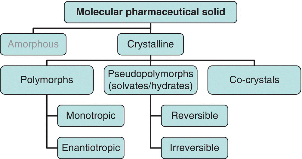
FIGURE 24.2 A map of the forms that a molecular pharmaceutical solid can exhibit. Crystalline materials are polymorphs, solvates/hydrates, and co‐crystals. Co‐crystals can be considered special cases of solvates, in which the “solvent” is instead an involatile compound that non‐covalently bonds to the molecular solid in a regular, ordered manner. Irreversible solvates can convert either to polymorphs, different solvates, or amorphous materials upon desolvation/dehydration.
Solid phases commonly exist as either “polymorphs” or “pseudopolymorphs.” Pseudopolymorphs are also referred to as solvates/hydrates. Polymorphism occurs when a single compound exists in two or more solid‐state forms that have identical chemical structures but that have different crystal lattice structures.
Polymorphs can have either “monotropic” or “enantiotropic” relationships. This behavior is exhibited in Figure 24.3. When two polymorphs have a monotropic relationship, they exhibit the same relative stability up to the normal melting point of both polymorphs. When an enantiotropic polymorphic relationship exists, the polymorphs change stability order at a transition temperature below the normal melting point of either polymorph. In Figure 24.3, the Gibbs free energy of polymorphs is shown for both a monotropic case and an enantiotropic case. For the monotropic case (b), the Gibbs free energy of form G1 is lowest across the temperature range until the melting point, where the liquid form of the material becomes most stable. In the enantiotropic case, Form G2 exhibits the lowest Gibbs free energy up to a transition temperature (Tp/st) at which point G1 exhibits the lowest Gibbs free energy. As the enthalpies of G1 and G2 do not change substantially up to the temperature range, this change in Gibbs free energy relationship is predominately due to the TΔS term.
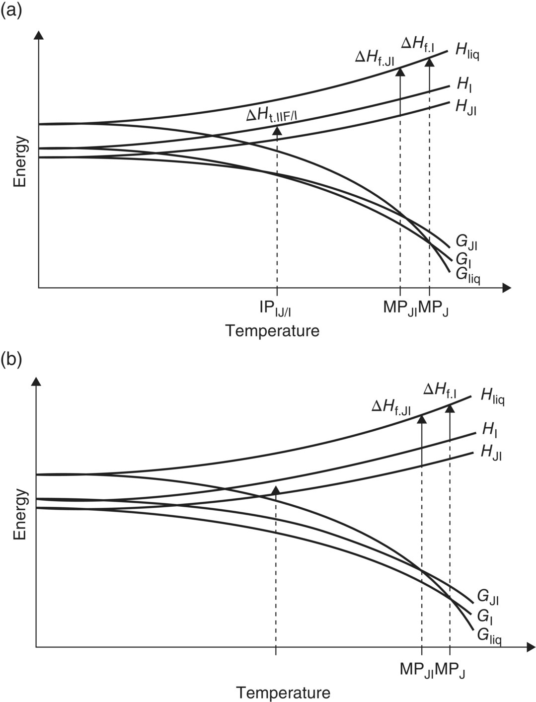
FIGURE 24.3 Thermodynamic description of polymorphism: enantiotropic (a) and monotropic (b) systems [5]. In the monotropic system, the stability order of forms is the same up to the melting point. For the enantiotropic system, a crossover temperature exists where the stability order changes.
Source: Reprinted with permission from Henck and Kuhnert‐Brandstatter [5]. Copyright (1999) Elsevier.
Solvates and hydrates occur when a solvent or water molecule is integrated into the crystal lattice through a repeating, non‐covalent bonding arrangement with the parent molecule. Co‐crystals are similar to solvates, except that a nonvolatile solute (e.g. nicotinamide [6], benzoic acid [7]) forms a regular non‐covalent, non‐ionic bonding pattern with the parent molecule. In the case of “reversible” hydrates and solvates, the molecule(s) of solvent/water can be removed from the pseudopolymorph without significantly affecting the crystallinity of the solid [8]. In some cases, amorphous solids can also be formed, typically through rapid precipitation, material comminution, or the desolvation of an irreversible pseudopolymorph.
Crystalline forms are important because they may exhibit different properties, some of which are listed below:
- Solubility
- Melting point
- Dissolution rate/bioavailability of a formulated solid dosage form
- Chemical and physical stability
- Habit and associated powder properties (for example, flow, bulk density, and compressibility)
As a result, the desired crystalline form is typically defined prior to initiating a crystallization design. For an intermediate, the form is often selected based on ease of manufacture, filterability, and chemical/physical stability. For a final product, it is often chosen based on performance in the formulated product (bioavailability, dissolution rate, chemical and physical stability) and on manufacturability in the formulation process (e.g. bulk density) [9, 10].
When designing a crystallization, it is frequently desired to produce the polymorph or crystalline form that is most stable at the solution composition and temperature prior to isolation. If the form being produced is not thermodynamically stable, it is possible for form conversion to occur at some point in the life cycle of the product, with the unstable form being difficult or nearly impossible to manufacture. An excellent example of this is the oft‐quoted ritonavir example, where a stable form appeared during commercial manufacture, causing a temporary disruption to supply, while the form issue was resolved [11]. Because the conversion from an unstable to a stable form is a kinetic process, it can be affected by changes in impurities, equipment, concentration, and process variables.
24.2.2.2 Particle Size
The second product performance criteria of concern is often particle size, although other properties such as surface area may be of equal or greater importance. The reasoning for the focus on particle size, and its frequent specification for APIs, is due to its potential impact on the performance of solid dosage forms:
- Particle size can affect exposure to patients and in vitro specifications such as product dissolution. Product dissolution for a drug tablet is a test where a tablet is stirred in an aqueous media with the aqueous media measured for drug content as a function of time. The test is used to ensure consistency between drug product batches and is often correlated to exposure levels in patients. For example, crystals with larger particle sizes often dissolve more slowly than small particle sizes, affecting the amount of material dissolved as a function of time.
- Particle size can affect final dosage form production by impacting powder conveyance and mixing, which can impact granulation (the drug product unit operation through which API is mixed with excipients, lubricants, and disintegrants prior to preparing the final dosage form, e.g. tabletting or capsule filling), and affect the uniformity of dose (the amount of drug in each dosage unit) and drug product appearance (color, shape, etc.).
For a detailed discussion of particle size and the nature of particle size distributions, thorough descriptions have been prepared [1]. Briefly, particle size distributions in pharmaceutical manufacture typically utilize mass‐ or volume‐based distributions. Mass distributions indicate what percentage of product mass is distributed into size intervals. Figure 24.4 displays a typical size distribution for a pharmaceutical, with references made to x90, x50, and x10. These values represent the particle size below which more than 90, 50, and 10% of the total mass of the product lie, respectively. Specifications for active ingredients most often contain a specification range for particle size that include one or more of x90, x50, and x10. While the example in Figure 24.4 reflects a measurement obtained through a laser light scattering method for particle sizing, alternative methods such as sieving are still routinely employed. Example Problem 24.1 illustrates a particle size determination problem.
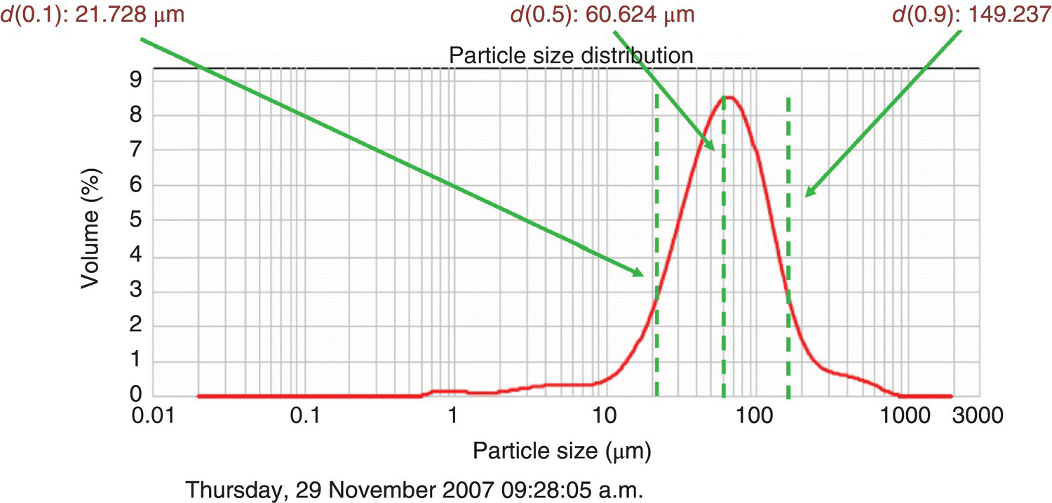
FIGURE 24.4 Particle size distribution (vol %) of a typical pharmaceutical product, measured by laser light diffraction. The d(0.9) or d90 corresponds to the size at which 90% of the area of the curve is contained.
24.2.2.3 Morphology and Powder Flow Properties
A knowledge of crystal habits is important in understanding the particle size distribution and the behavior of powders and slurries, as different crystalline habits have different characteristic lengths and different flow characteristics. Flow characteristics are important because poor flowing powders can influence the ability of a powder to blend with excipients into a uniform granule and can also impact the flow of powder through primary and secondary unit operations, causing phenomena such as “rat‐holing” in powder feed hoppers.
Figure 24.6 displays a summary of common habits observed in pharmaceutical crystallizations. Equant/block habits typically result in products that are easy to isolate, dry, and handle, due to their relatively low surface area/volume ratio. Acicular and thin blade crystals, which are common in pharmaceuticals, tend to pose more processing difficulties, such as long isolation times, agglomeration, and poor flow and handling properties. Despite processing difficulties, these habits may also result in high surface area materials, which can positively impact bioavailability performance in a formulation.
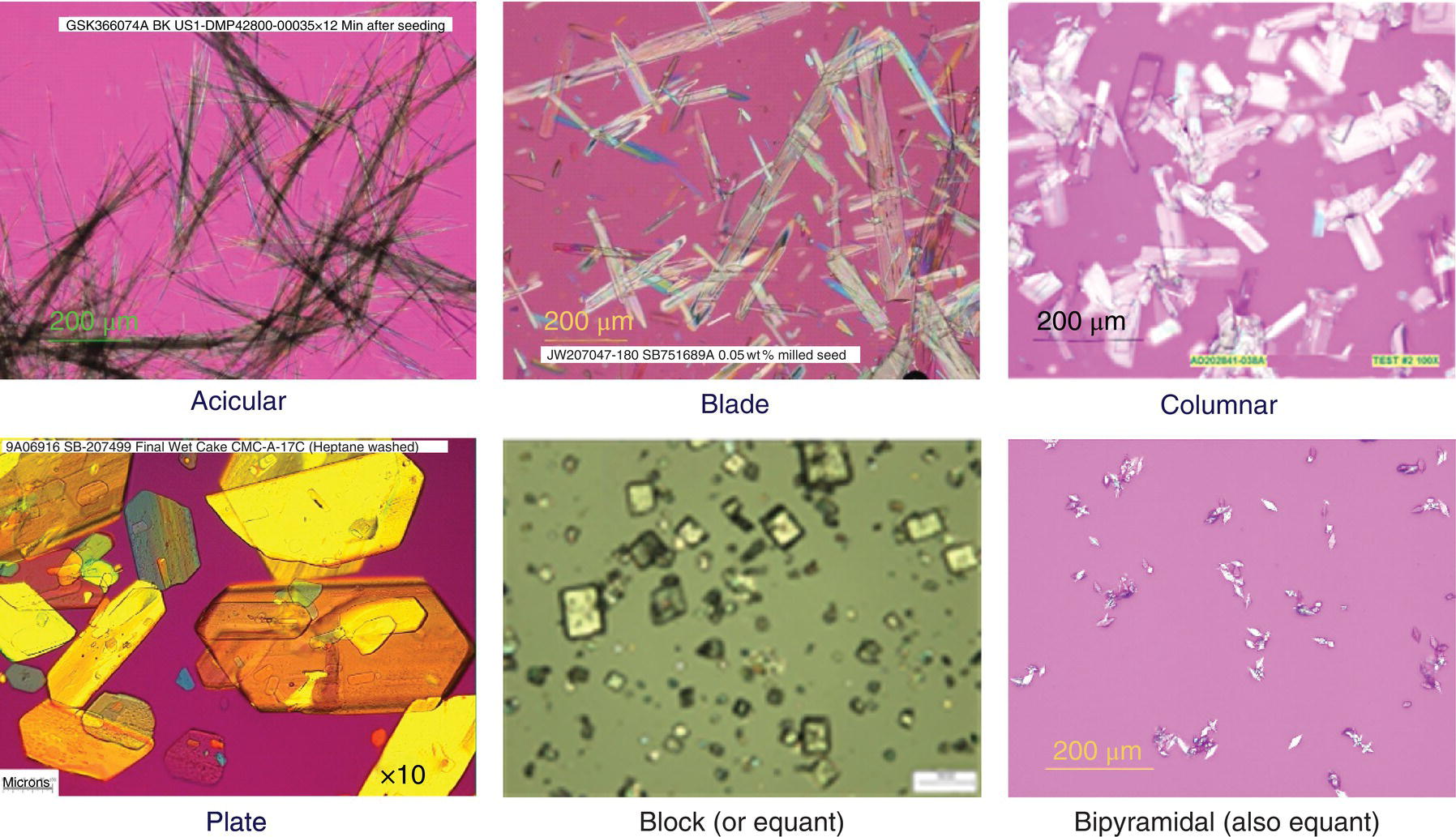
FIGURE 24.6 Commonly observed habits in pharmaceutical crystallization. For a more complete description of habits, please see Ref. [1].
The flow characteristics of a powder are frequently inferred from knowledge of powder densities, commonly the bulk and tapped density. The bulk density of a powder is the density measured “as is,” while the tapped density uses mechanical “taps” to facilitate further packing and settling of the powder. The ratio of the tapped to bulk density is referred to as the Hausner ratio and provides an indication of the compressibility of powders and as a result the ease of powder conveyance. Materials with a Hausner ratio of less than 1.2 are generally considered to have good flow properties, while those with a ratio greater than 1.4 are considered to have poor flow properties. The absolute values of density are also important, as they affect the level of fill for a piece of equipment. If material A has twice the bulk density of material B, the size of a batch can potentially be twice as large, resulting in throughput savings. Acicular materials routinely have Hausner ratios > 1.3 and bulk densities < 0.2, while block and equant habits often have bulk densities > 0.3 and Hausner ratios < 1.2 [12]. In addition to habit, particle size plays a strong role in affecting material bulk densities.
24.2.3 Manufacturability
Common manufacturability criteria include yield, cycle and batch times, environmental impact, and processability. Theoretical process yields are calculated with equilibrium solubility data and are described in the next section. Cycle time is affected by the time it takes for the crystallization to proceed and by the time spent in the isolation and drying unit operations. For instance, a crystallization can require a long time to maximize particle size, resulting in short isolation and drying times, or the crystallization can occur quickly, resulting in a short crystallization time with small particle generation causing long isolation times. The integration of crystallization, isolation, and drying must be considered to deliver an optimum throughput for a product. An example of batch time analysis for a crystallization and isolation process is shown in Example Problem 24.2.
Example Problem 24.2 illustrates a key aspect of crystallization design, which is shown in Figure 24.8. The crystallization in the example affects isolation performance, which in turn affects drying performance, which affects sieving and size reduction performance, which ultimately affects performance in the formulation process. As a result, it is often necessary to study crystallization in conjunction with several unit operations. As shown in Example Problem 24.2, it is straightforward to assess the dependence of the crystallization on the isolation step, and the drying step can further be integrated into structured studies. Each downstream unit operation must be investigated for its impact in ensuring the process, and not just the crystallization, achieves the desired performance objective.
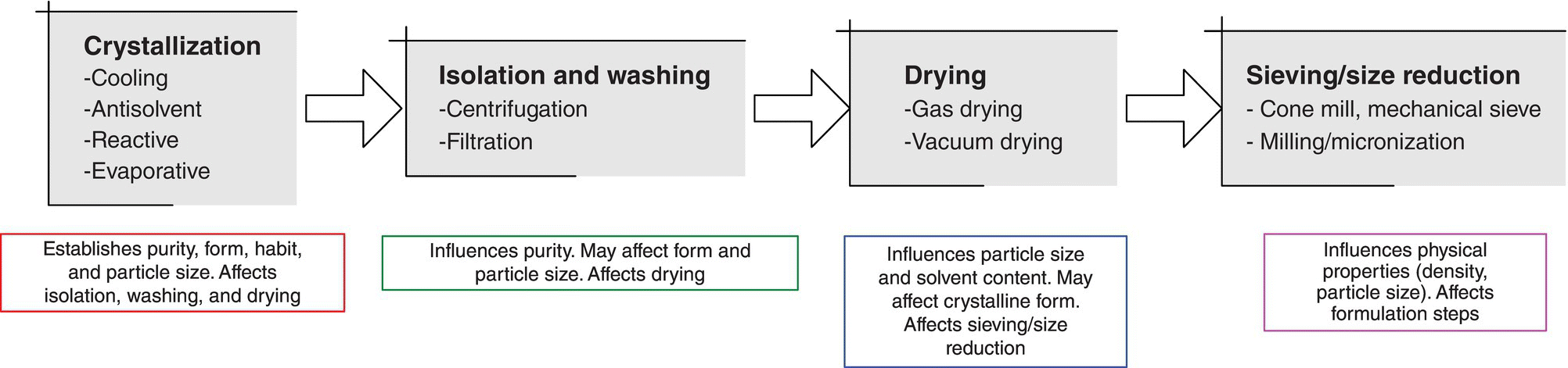
FIGURE 24.8 The relationships of crystallization with downstream processing steps. Crystallization typically needs to be studied in conjunction with downstream steps to understand the complete control of desired attributes.
24.3 SOLUBILITY ASSESSMENT AND PRELIMINARY SOLVENT SELECTION
An understanding of a compound’s solubility is the normal starting point for crystallization design. The solubility of a compound determines the throughput and yield; it is often the key property in selecting a solvent system and designing the crystallization procedure. Coupling the API solubility with the solubility of impurities can assist in predicting selectivity or impurity purging.
Solubility is a thermodynamic property of a solute that describes the equilibrium of a defined solid phase (e.g. a polymorph, pseudopolymorph, or other) with a solution, as shown in Eq. (24.2). It is a dynamic equilibrium whereby the rate of dissolution is balanced by the rate of crystallization:
Solubility is determined through equilibrium experiments in which a solid phase is slurried isothermally with a solvent until a constant concentration is achieved in the solution phase. Typical solubility data for a pharmaceutical compound is shown in Figure 24.9. This data illustrates the general approach to data measurement: solid of a known phase is added to a predefined amount of solvent at low temperature, an equilibrium concentration is achieved, and the temperature is then increased, ensuring solids are still present. At the end of the experiment, the solid phase of the material is assessed to ensure the crystalline form has not changed, as different forms have different solubility equilibria. If binary or ternary solvents are being studied, the phase composition of the mixture should also be measured at the end of the experiment to ensure no changes. Each compound possesses its own time scale in which equilibria are achieved. This typically ranges from minutes to several hours, although days are required in some circumstances. As illustrated in Figure 24.10, in‐line methods of solute concentration measurement are useful in understanding time to equilibria. When in‐line methods are not practical, measurement of the filtered equilibrium solution by HPLC (or gravimetric analysis if the material is relatively free from impurities) is commonly used.

FIGURE 24.9 Results from a solubility experiment using diamond attenuated total reflectance IR spectroscopy to measure concentration in situ for a pharmaceutical active ingredient. At increasing temperatures, the solute achieves an equilibrium in the different solvent mixtures, indicated by the plateau in concentration upon achieving a new temperature. In this case, equilibrium is rapidly achieved.

FIGURE 24.10 Solubility data from Figure 24.9 regressed using a simple van’t Hoff relationship. For some solvents, the fit is very linear (e.g. tert‐butyl methyl ether). Other solvents would benefit from an additional fitting parameter due to curvature (e.g. toluene using the C ln(T) term).
While Figure 24.10 displays solubility as a function of temperature, it may also be measured as a function of solvent composition. When temperature is used to generate solubility differences, the result is a “cooling” crystallization. When solvent composition is used, the result is often called an “antisolvent” crystallization. In all cases, the preferred units of solubility are mass solute/mass solvent. Using these units simplifies subsequent engineering calculations.
Once data is collected, it can be evaluated for use in process design. The thermodynamic description of two phases in equilibrium is
From this, one can derive an expression for solubility of the general form

where
- xi is the solubility of the drug, mol drug/mol solution.
- γdrug is the activity of the drug in solution.
- ΔHtp is the enthalpy change for a liquid solute transformation at the triple point.
- ΔCp is the difference in CP of the liquid and solid drug.
- ΔV is the volume change.
- T, Ttp is the temperature, triple point temperature.
- P, Ptp is the pressure, triple point pressure.
- R is the universal gas constant.
In almost all situations, pressure has little to no effect on solubility; therefore the pressure term can be eliminated. The change in heat capacity is often assumed to be negligible, and the triple point is often replaced with the melting point of the solid to yield the approximation shown in the equation below:
For an ideal solution, this can be reduced to a van’t Hoff type expression and linearized
where
- Ssolute is the observed solubility.
- As and Bs are constants obtained by linear regression.
For ease of use in future calculations, ln(S) is typically taken with S having units of mass of API per mass of solvent and temperature having units of Kelvin.
The linearization is similar for nonideal solutions with the exception that Bs becomes
The consequence of a nonideal solution is that Bs becomes a function of temperature and solvent composition.
Almost all solutions containing a high fraction of API are nonideal; however this linearization technique (plotting ln S vs. 1/T) is a simple way to visualize and interpolate solubility from a few data points. For systems in which these plots are nonlinear, a correction can be added to Eq. (24.6a) by including a [+C ln(T)] term [1]. In other cases, polynomial functions may be used to represent data, but these expressions tend to be less representative when extrapolated beyond the range of temperature studied in the solubility experiment.
Once solubility is measured, it can be used for a number of purposes. First, it can be used to select the crystallization solvent based on the constraints of the system, typically yield, throughput, and environmental constraints. The yield in particular is often estimated by Eq. (24.7):
In Eq. (24.7), S1 and S2 are the solubilities at the dissolution temperature and composition and the solubility at isolation temperature and composition, respectively, and m1 and m2 are the mass of solvent at the dissolution temperature and composition and the mass of solvent at isolation temperature and composition, respectively.
Another use of solubility data is the estimate of purification potential of a crystallization. To perform this assessment, the solubility of the impurity must also be known. Using Eq. (24.7), it is then a straightforward calculation to calculate the mass of impurity and desired solute out to estimate the potential for the crystallization to achieve purification goals. The actual purification can be less than the calculated values due to impurity inclusion or occlusion in the product. The following example illustrates the use of solubility data to estimate the purification potential of a solvent.
24.4 CRYSTALLIZATION KINETICS AND PROCESS SELECTION
Solubility, like any thermodynamic relationship, provides a starting point and an endpoint for a process. Knowledge of crystallization kinetics is critical in determining the path through which the beginning and endpoint are linked. For chemical reactions, kinetics is used to indicate the rate of change of molecular species; for crystallizations, kinetics is used to indicate the rate of solute mass transfer from solution phase to a solid phase. While solubility is often a primary control for achieving purification and separation objectives, the kinetic mechanisms of a crystallization are typically the primary determinant for physical properties. Readers are referenced to more comprehensive discussions on these topics, for example [3].
Following the preliminary selection of one or multiple solvents from solubility data, the kinetics of the system must be understood in order to choose the conditions under which the crystallization operates and to validate the choice of solvent. If the chosen solvent presents significant challenges related to kinetics that prevent the crystallization from achieving its design objectives, a new solvent is often sought.
Essential to understanding the kinetics of crystallization is the concept of supersaturation, which is the driving force for common crystallization mechanisms. Common expressions of supersaturation are shown by the equations presented below:
In the equations above,
- C is the actual concentration of solute at a reference point.
- S is the equilibrium solubility at the same point.
- σ1 is the supersaturation in absolute terms (concentration).
- σ2 is referred to as the supersaturation ratio.
- σ3 is referred to as the relative supersaturation.
All three terms are frequently used in the analysis of crystallization processes.
Crystal mass is generated by either nucleation or growth. Nucleation can be described as the formation of new crystals from a solution or slurry, while growth can be defined as the deposition of solute mass on existing crystals of that solute. Nucleation can further be divided into two mechanisms: “primary” nucleation, which is the formation of new crystals from solutions devoid of crystals, and “secondary” nucleation, which is the formation of new crystals in the presence of existing crystals. Primary nucleation can occur within solutions (homogeneously) or at surfaces (heterogeneously, e.g. on crystallizer walls, agitators, etc.).
Nucleation generates small crystals, which can be useful in preparing small particle size powders. However, nucleation can also lead to significant downstream processing problems, such as long isolation times, significant agglomeration leading to poor performance in a formulation, and batch‐to‐batch variability. Crystal growth is used to increase the size of the product, reduce batch‐to‐batch variability, and overcome downstream processing and handling issues [15]. It is also used to control the crystalline form of the compound being prepared for systems in which multiple forms may nucleate. As a result of the benefits afforded by crystal growth, it is generally preferred as the dominant mechanism in crystallization design, especially for controlling physical properties of materials.
24.4.1 Nucleation Kinetics and the Metastable Limit
When solutions are supersaturated, they are thermodynamically unstable. Like chemical reactions that do not react spontaneously, a thermodynamically unstable solution does not necessarily crystallize spontaneously as an energy barrier must be overcome to form a surface, analogous to the activation energy associated with a chemical reaction. Solutions that are supersaturated but do not spontaneously crystallize are referred to as “metastable.” A complete description as to the origin of metastable solutions can be found in Ref. [1]. It is quite common for pharmaceutical intermediates and APIs to form metastable solutions at supersaturation ratios between 1.0 and 1.2. Eventually (weeks to years), many “metastable” systems might nucleate, but over the time scales associated with processing (minutes to hours), nucleation typically does not occur. A solute is said to be at its metastable limit when it is at the maximum supersaturation at which primary nucleation does not spontaneously occur.
After the solubility, the metastable limit is the next critical measurement in crystallization design. It is measured by two primary methods, which are described in detail in Table 24.4.
TABLE 24.4 Description of Metastable Limit Measurement Techniques
| Method | Description |
|
|
|
|
An example of metastable limit determination and data reduction is provided by Example Problem 24.4 for a cooling crystallization and an antisolvent crystallization.
Of the two methods for estimating metastable zone width, the nucleation induction time method is often the most general, as it is broadly applicable to all crystallization modes. In addition, the nucleation induction time method gives an indication of the time window that is available to allow the addition and growth of seed materials and mix antisolvents/reactants with the main solvent. The nucleation induction time is also useful in understanding the scale‐up implications of crystallizations and is described later in this chapter.
While the metastable limit is useful in understanding the conditions under which primary nucleation occurs, the potential for secondary nucleation must also be considered. Secondary nucleation occurs through several mechanisms, with the most common mechanism being contact nucleation. Contact nucleation is micro‐attrition of crystals, resulting in small crystalline fragments (<10 μm) being present in the slurry [16]. The rate of contact nucleation is influenced by crystal–crystal, crystal–impeller, and crystal–wall collisions. A common expression for contact nucleation is indicated by Eq. (24.14):
where
- B is the nucleation rate in number per volume per time.
- M is the suspension density in number (expressed as mass per volume).
- N is the agitation rate (expressed as a frequency or a velocity).
Secondary nucleation can occur within the metastable limit.
24.4.2 Growth Kinetics
Crystal growth theory and mechanisms have been well described in several references. For the practicing engineer working on design and scale‐up issues, this discussion is simplified below into the content that is typically required to analyze commonly used pharmaceutical crystallization modes.
Like nucleation, crystal growth is driven by a supersaturation driving force, with Eq. (24.15) illustrating a commonly used rate expression:
where
- kGM is a temperature‐dependent rate constant.
- Ac is the surface area of solids present in solution.
- γ is the order of growth.
- m is the mass of solute.
Growth occurs either on material that has already been generated by nucleation or on material that has been purposefully added to the solution. Purposefully added material is referred to as “seed.” Seeding is frequently employed in pharmaceutical crystallization processes to control crystalline form and physical properties, especially particle size. Seed material may be prepared from an alternative processing method, such as milling, or may be taken from one batch of material and added to a subsequent batch.
If a system exhibits growth as the primary mechanism for crystal mass formation, the amount of seed added controls the particle size of the product. A common expression used to interpret the relationship of seed amount to particle size for batch crystallization processes is expressed by the proportionality shown below:

In the proportionality,
- ms represents the mass of seed.
- mp represents the mass of product.
- ds and dp represent sizes of the seed and product, respectively.
Typically, d50 or d90 values from laser light diffraction measurement or sieve measurement are used for the size terms. The exponent term n is related to the morphology of the crystal. For a perfectly spherical crystal, the exponent n would equal 3, and the proportionality would be an equality. In practice, the relationship between seed amount and particle size at the end of the crystallization is obtained by an empirical regression of the seed response curve (prepared by running the process at several seed loading [ms/mp] values and trending versus product size for several seed types). The preparation of seed response curves and subsequent analysis is described by Table 24.6.
TABLE 24.6 Method for Generation of Seed Response Curves
| Step Number | Description of Step |
| 1 |
|
| 2 |
|
| 3 |
|
| 4 |
|
After generation of the seed response curve, the amount and size of seed required to deliver a desired particle size can be interpolated from the resultant data/correlations. When conducting these experiments, it is important to conduct the experiments at supersaturations within the metastable limit, so that growth is the predominant mechanism. An example of a seed response curve is illustrated in Figure 24.14.
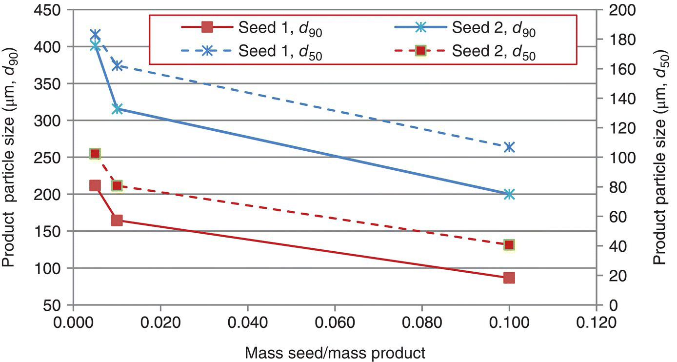
FIGURE 24.14 Typical seed response curve plot. Seed 1 in this case has a d90 value of 6.1 μm and a d50 of 2.2 μm, while Seed 2 has a d90 of 11.5 μm and a d50 of 4.4 μm. Both d90 and d50 values exhibit the anticipated response.
In performing seed response curve experiments, the kinetics of crystal growth can also be measured. Growth kinetics are valuable in crystallization design, as they can be used to determine the required rates of cooling, antisolvent addition, distillation, and reagent addition for the corresponding crystallization mode. Many methods for the measurement of crystal growth kinetics can be used [2, 3]. One useful method for growth kinetics determination in batch systems is through the measurement of solute concentration as a function of time following the addition of seed to a supersaturated solution. Varying the seed amount changes the “area” term in Eq. (24.15), allowing the determination of the rate constant. The area term is often indicated using a “specific surface area” measurement determined through nitrogen adsorption methods or by understanding the size distribution of a material and the shape factor through which an area of a material can be related to its mass or characteristic length. Measurement of the rate constant as a function of temperature enables a correlation over the entire path of a crystallization.
Figure 24.15 displays a typical crystal growth kinetic experiment and associated data fit. For this particular case, an online method (measurement of concentration by reflectance infrared spectroscopy) was used to measure solute concentration. The solute concentration data was used to calculate supersaturation at each time point. The initial conditions for the solution of Eq. (24.15) were t = 0, C = 0.094 kg solute/kg solvent (1 l of solvent used; density of the solvent = 800 kg/m3) with the solubility at the experimental temperature being 0.074 kg solute/kg solvent. The data was adequately fit through numerical integration using a simple finite differences method and a sum of square residual minimization to estimate a value for kGM A = 1.6 × 10⁻⁶ m3/s. With a seed area of 0.116 m2, kGM = 1.4 × 10⁻⁵ m/s. Due to the relatively small change in mass over the experiment, the value of Ac was approximated to be constant during this experiment. A more rigorous solution would relate mass change to area change either through the use of a shape factor or an empirical correlation, or alternatively an initial rates method would be used with a constant area approximation. Crystallization growth rate orders are often low, with values between 0.5 and 1. In the experience of the authors, a large number of pharmaceutical systems exhibit reasonable growth model fits with when assuming first order in supersaturation.

FIGURE 24.15 Crystal growth kinetics from concentration data. Crystallization seeded at time 0. Details are provided in the text. A finite differences approach was used to solve for the growth rate constant, kGM = 1.4 × 10⁻⁵ m/s, with seed surface area Ac = 0.116 m2 and solvent volume Vsolvent = 1 l.
24.4.3 Controlling and Determining Crystallization Mechanisms
Figure 24.16 summarizes the kinetic discussions above by displaying regions of concentration in which different mechanisms are likely to occur for either cooling or non‐solvent crystallizations. To maximize the opportunity for crystal growth, operation in close proximity to the solubility is preferred. The nearer the solution concentration is to the metastable limit, the likelihood of secondary nucleation is increased, with primary nucleation possible at concentrations beyond the metastable limit. The principles in Figure 24.16 are applicable to evaporative and reactive crystallizations, but in these situations supersaturation is typically generated by changes in concentration rather than solubility.
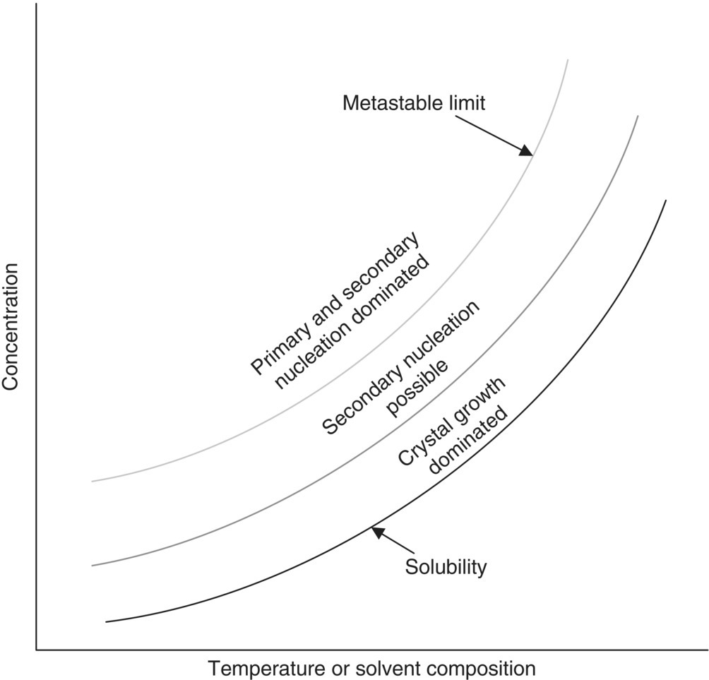
FIGURE 24.16 Mechanisms of crystallization and their relationship to solute concentration. Primary nucleation predominates when the solution is supersaturated beyond the metastable limit. Secondary nucleation can occur within the metastable zone, typically at supersaturations near the metastable limit. Growth frequently is the dominant mechanisms at relatively low supersaturations (i.e. concentration is close to the solubility).
Crystallization mechanisms are inferred from experimental data, especially microscopy and solute concentration data. From a design perspective, conditions are sought, which provide the balance of mechanisms required to deliver the objectives of the crystallization. In Figure 24.17, successive micrographs are taken after seeding a pharmaceutical product within the metastable zone. As observed in the figure, the seed materials grow successively larger with time with no new fine crystals are observed. This is the type of behavior representative of a growth‐dominated system and indicates that the crystallization is operating sufficiently close to the solubility curve to minimize secondary nucleation.
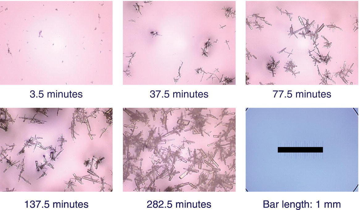
FIGURE 24.17 Illustration of crystal growth mechanism observation by optical microscopy. The processes is seeded at time 0 with the process held isothermally for 282.5 minutes. Fine particles disappear as coarse particles appear, which grow larger throughout the duration of the experiment with no evidence of fine reappearance [17].
Source: Reproduced with permission of Elsevier.
In Figure 24.18, micrographs are overlaid with solute concentration data for a system that exhibits both growth and secondary nucleation. The solution was supersaturated beyond the metastable limit before adding seeds. Some crystal growth is observed immediately after seeding. After a growth period where seed material has clearly disappeared and been enlarged through growth, a change is seen in the slope of the solute concentration curve, indicating a mechanism change from growth to nucleation. Upon further desupersaturation, the crystals have not grown larger, and the habit has slightly changed from a columnar habit to more of a thin plate habit (the form has not changed). The change in the rate of desupersaturation combined with the change in crystal habit and the lack of crystal enlargement is clear evidence of secondary nucleation.
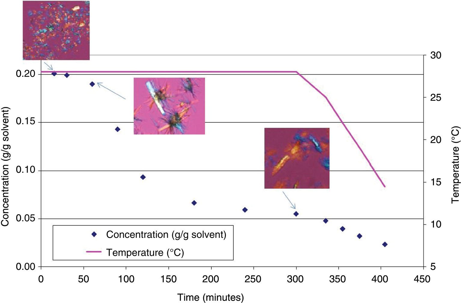
FIGURE 24.18 A crystallization experiment exhibiting both growth and secondary nucleation mechanisms. Initially, seeds grow as indicated by the presence of large crystals shortly after seeding. With additional time, a change in slope during desupersaturation is observed, indicating a change in mechanisms to secondary nucleation.
Of particular use in mechanism detection are process analytical instruments that detect particulate matter, such as in‐line microscopy or LasentecTM focused beam reflectance microscopy. Overviews of the utility of FBRM in crystallization mechanism inference can be found at [17].
When considering a design for a crystallization that will encourage growth, a recommended starting point for a design is to add seed at a concentration no more than midway between the solubility curve and the metastable limit and to maintain this minimum proximity to the solubility curve for the remainder of the crystallization process. Initial experiments are performed using microscopy, concentration, and online particle detection methods to ensure the selected conditions are indeed producing the desired mechanism. Conditions are then verified at larger scale to ensure that changes in mixing or equipment geometry and materials of construction have not altered the mechanistic behavior. Acicular habits, in particular, are highly prone to contact nucleation as they can easily be broken.
While crystal growth and nucleation are most frequently observed mechanisms, other important mechanisms are possible. These include oiling and aggregation or agglomeration. In the case of oiling, supersaturation is typically in great excess of the metastable limit or the solution sufficiently concentrated with nucleation inhibiting impurities that the solute forms a liquid phase consisting of a solvent–solute concentrate rather than a stable crystalline form. Oils are metastable and may crystallize spontaneously with sufficient holding times. Aggregation occurs when two crystals collide in solution and adhere to each other through surface–surface interactions. Once an aggregate forms, it can either be disrupted with the crystals regaining their individual identity (this typically occurs through fluid shear), or the crystals may fuse together due to growth that links the two surfaces. When crystals fuse together, the result is frequently called an agglomerate. Aggregation is often severe in processes in which nucleation occurs at high supersaturations and is common for acicular habits or for crystals with high specific surface areas. Severe aggregation is often manifested as an immobile slurry that does not mix well and under certain conditions can result in “shelves” of solid on internal reactor equipment. As aggregation and agglomeration can affect processability, physical properties, and mixing scale‐up, the approach is often taken to minimize supersaturation to reduce the driving force for aggregate or agglomerate formation. In certain instances, aggregation or agglomeration is purposefully attempted to prepare a material that behaves like a small particle from a pharmaceutics perspective (e.g. rapid dissolution in a dosage form) but behaves like a larger particle from a manufacturability perspective (e.g. short filtration times). Examples of the favorable use of aggregates or agglomerates include spherical crystallizations [18]. The design of a spherical crystallization process is highly dependent on the properties of a molecule and often must be established on a trial‐and‐error basis.
24.5 APPLICATION OF SOLUBILITY AND KINETICS DATA TO CRYSTALLIZATION MODES
The kinetic and thermodynamic principles described in the previous sections can be applied to common crystallization modes to complete a batch or semi‐batch crystallization design. For most situations, it is recommended to pursue a design where growth is the dominant mechanism, as such processes are simpler to reproducibly scale‐up from a heat and mass transfer perspective. To enable a growth basis for design, seeding is employed to provide the initial area required for growth. This is especially the case for active ingredients where control of particle size and crystalline form are the key objectives. When tight control over physical properties is less of an issue, a preferred design approach may be to nucleate at a constant but small supersaturation (e.g. just outside of metastable limit) and then grow the nuclei at a supersaturation within the metastable limit.
These two design methods are illustrated in Figure 24.19 for common crystallization modes. In Figure 24.19b, d, and f, the crystallization is seeded within the metastable limit, and supersaturation is maintained within the metastable limit until the crystallization has completed. This approach provides the best opportunity to maximize the potential for crystal growth, although it is possible to have some secondary nucleation. In Figure 24.19a, c, and e, nucleation is induced by increasing the supersaturation beyond the metastable limit, but supersaturation is then controlled to ensure that the rest of the crystallization occurs close to the solubility line.
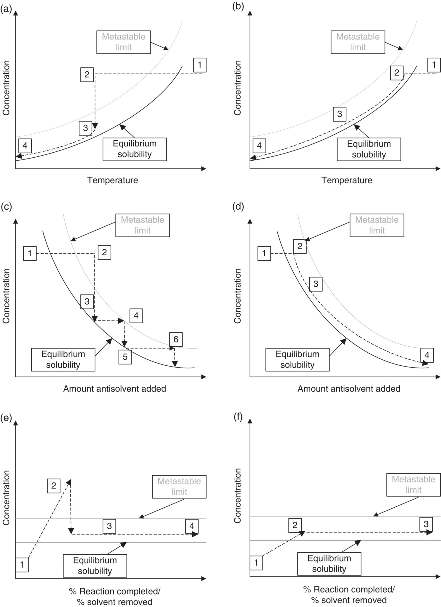
FIGURE 24.19 Frequently used crystallization design modes in pharmaceutical processes. (a) and (b) represent cooling crystallizations, (c) and (d) represent crystallizations induced by antisolvent addition, and (e) and (f) represent both reactive and evaporative crystallizations, which can be similar in terms of behavior. (a), (c), and (e) represent situations where initial crystal mass is generated by primary nucleation, with growth occurring after the nucleation event through controlled generation of supersaturation. The amount of nucleation is dependent on how much supersaturation is generated prior to crystallization. (b), (d), and (f) represent seeded crystallizations, where seed is added in the metastable zone. In each plot, (1) represents the starting point of the crystallization, where all material is dissolved. (2) represents the point at which crystallization mass is first generated, either by seeding or by nucleation. The highest number on each plot represents the point at which the crystallization is complete.
A common error in crystallization design and scale‐up is the generation of supersaturation to levels where nucleation is a dominant mechanism. This is caused by a lack of understanding of the time scales over which controlling process parameters need to be changed. This section addresses simple approaches to estimating the time scales for the controlling parameters in each major crystallization mode:
- Rate of temperature change (cooling crystallizations).
- Rate of addition of antisolvent (antisolvent crystallizations).
- Rate of reaction through control of temperature or addition of reactants (reactive crystallizations).
- Rate of solvent removal (evaporative crystallizations).
Only simple methods for the estimation of process parameters are provided. There are many published examples of more rigorous approaches to solving similar problems, particularly the work of the Bratz1 and Rawlings2 research groups, which are recommended for further study.
24.5.1 Cooling Crystallization
Seeded cooling crystallizations represent perhaps the simplest design approach for achieving consistent crystallizations while minimizing scale‐up challenges. The challenge is to balance the growth rate with the rate of supersaturation generation. In order to understand the required rate of change of temperature to meet this objective, a knowledge of crystal growth kinetics for the seed material and amount planned to be used in the crystallization are required (Figure 24.15).
The growth rate is balanced with the rate of supersaturation generation through cooling such that the process remains within the metastable limit and near the solubility line. A simple approach to achieving this condition is achieved through the use of Eq. (24.17), where the growth rate is expressed both in terms of the solid phase (dm/dt) and the solution phase (Vsolvent(dC/dt)):
Through knowledge of the metastable limit and nucleation induction times, a supersaturation is selected at which the material is desired to grow. Typically, this is a concentration within the metastable limit and close to the solubility line. The exact value selected is dependent on the compound and its propensity for secondary nucleation within the metastable limit. Two operational methods are employed. Method 1 involves supersaturating to a selected value, seeding, and initiation of a cooling profile soon after seeding. This method can be problematic if there is sufficient statistical variation in the process such that the planned supersaturation is actually not achieved. For instance, if a solution is saturated at 70 °C, and the selected seeding temperature is at 68.5 °C, but the temperature probe has an error of 2 °C, and the solvent charge has an error of 1%, seed materials may dissolve. Method 2 is more commonly employed and involves seeding at a supersaturation within the metastable limit but at a level where the typical processing errors that cause seed dissolution are highly improbable. After seed growth desupersaturates the solution to an acceptable supersaturation, further supersaturation generation can be achieved through cooling.
Equation (24.17) can be solved with simple numerical solutions to determine both the time required for seed to desupersaturate a solution through growth and for the cooling rates after the initial desupersaturation. This is illustrated in Example Problem 24.5.
In the event that seeding is not practical or for the case of intermediates, an alternative possibility is to cool to a point outside of the metastable limit, nucleate at a constant supersaturation, and then control the subsequent cooling in order to maximize crystal growth. The same methodology shown in Figure 24.5 is applicable for the subsequent growth phase, except that the nucleated material must have an estimated area in order to apply a growth kinetic model.
24.5.2 Antisolvent Crystallization
The rate of antisolvent addition to maximize growth potential can be calculated through a similar approach to that described for a cooling crystallization. In this case, the volume is not constant but varies with volume, resulting in Eq. (24.18):
The addition rate curve will depend on the shape of the solubility curve but typically will be similar to a cooling crystallization in that the addition rate will at first be slow and will ramp up near the end of the crystallization [19]. As with a cooling crystallization, the first step is to add antisolvent to generate a supersaturation within the metastable limit and then calculate the time needed to desupersaturate for a given seed load. The next step is then to calculate the rate of antisolvent addition. This can be done through a numerical integration of Eq. (24.18). It is first necessary to select a supersaturation appropriate to maintain crystal growth using metastable limit data. A simple finite difference approach involves starting at this supersaturation and calculating the growth rate at this supersaturation. The volume is then incremented in small intervals, with the change in solute mass calculated over each volume interval through the difference of the solubility times the mass of solvent across the volume interval. The time required for each added increment of antisolvent is calculated by dividing the change in mass over a time interval by the growth rate. The results of such a calculation are shown in Figures 24.20c and d for a system in which water is added to a methanol solution containing an active ingredient, again assuming that kGM A is constant over the entire crystallization (0.6 g/min). For this particular scenario, the solvent is methanol and the antisolvent is water. The solubility of the binary system is described by an exponential function, S = 0.22 exp(−12.04 ϕwater), where ϕwater is the water volume fraction. Initially, 1 kg of material is dissolved in 6 l of methanol, and 0.15 l of water is added to generate supersaturation at 20 °C. The solution is then held until a supersaturation of 0.004 g/g solvent is achieved. Antisolvent is then added at a rate such that this supersaturation is maintained to achieve a total added volume of 4.25 l. The result is a seed hold time of approximately 24 minutes and a total addition time of approximately 317 minutes. The shape of the addition curve mirrors the solubility as a function of water volume fraction. As with the cooling crystallization, nucleation can also be used to initiate the crystallization, with growth rates calculated after understanding the area nucleated.
24.5.3 Reactive Crystallization
In most cases, reactive crystallizations are of interest when the product of the reaction is negligibly soluble and the crystallization rate is typically the rate‐limiting step. For these systems, the challenge is to match the rate of product generation with the rate of crystal growth so that excess supersaturation is not generated. For a simple bimolecular reaction, where {A + B → Product}, the following rate balance can be written as:
The rate of reaction for many pharmaceutical applications can be controlled by the rate of addition of reactant, resulting in the volume (V(t)) being a function of addition rate and time. In the simplest instance, the reactant of interest is an ionizable compound that forms a salt with the pharmaceutical molecule. In this situation, the rate of reaction is essentially instantaneous with the addition of the reactant and can control the generation of supersaturation.
An example of a common pharmaceutical synthesis reaction is shown in Figure 24.21. This is a Boc deprotection reaction with an acid reactant. Upon deprotection, the resultant species is able to form a salt with the acid reactant, which has limited solubility in the reaction solvent. A numerical solution to Eq. (24.19) is illustrated in Figure 24.22a for this example.
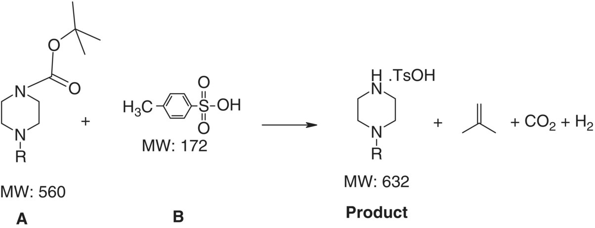
FIGURE 24.21 Reaction scheme as an example of a reactive API crystallization process.
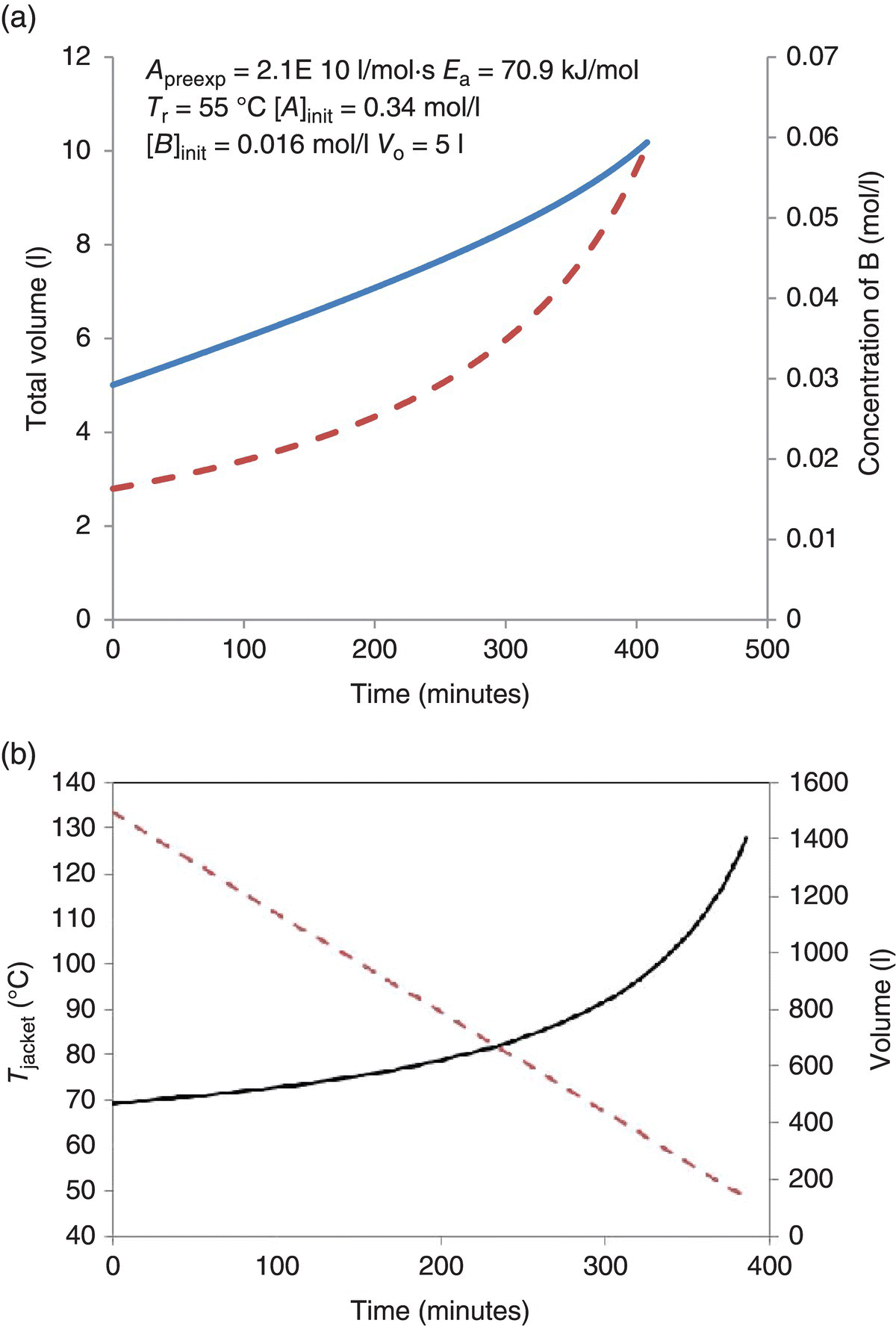
FIGURE 24.22 Examples illustrating constant supersaturation control for (a) reagent addition for a reactive crystallization and (b) jacket temperature for an evaporative crystallization. The reaction for (a) is shown in Figure 21, run isothermally at 55 °C (Ea = 70.9 kJ/mol, Apreexp = 2.1 × 10¹⁰ l/mol s). Starting amount of compound A is 1 kg in 5 l solvent. Initially, the reaction was run to approximately 5% completion, through an addition of 5 mol % compound B, and a product concentration of 0.004 g/g solvent was achieved after seeding and seed growth. The balance of B was then added in a feed solution with a concentration of 0.336 mol/l. Compound B was added such that a supersaturation of 0.004 g/g solvent was maintained. kGM Ac = constant = 9.8 × 10⁻⁶ m3/s. For (b), the solvent was distilled from 1500 to 100 l; kGM Ac = constant = 2.9 × 10⁻⁴ m3/s. The vessel has a linear correlation between surface area and volume Avessel (m2) = 0.003 22 Vsolvent + 0.53. The overall heat transfer coefficient was 340 W/m2 K, the solvent was methanol, and the supersaturation upon seeding was 0.005 g/g solvent; this was maintained throughout the crystallization.
24.5.4 Evaporative Crystallization
In evaporative crystallization, the solubility is constant, so the rate of supersaturation generation is proportional to the amount of solvent mass removed (dm/dV):
For a constant supersaturation, this equation is trivial to solve. A constant boilup rate is necessary to maintain a constant supersaturation. The complication arises during scale‐up. As the volume decreases in the reactor, the effective heat transfer area decreases, thereby changing the temperature required on the jacket to maintain the constant boilup rate (Figure 24.22b).
24.6 ADVANCED TOPICS
24.6.1 Obstacles to Crystallization
24.6.1.1 Polymorphism and Solid Phases
Polymorphism is the property defined as the ability of a molecule to exist in multiple solid crystalline phases that have different molecular spatial arrangements and/or conformations [20–22]. Polymorphism often arises from molecular flexibility and different patterns for self‐assembly. Different polymorphs (crystalline phases of the same molecular entity) often exhibit different crystal lattice characteristics that result in different macroscopic properties and behaviors such as crystal habit, growth and nucleation kinetics, solubility, dissolution rate and powder flow, and cohesivity. Polymorphs of the same substance are typically ranked in terms of stability with one isolated polymorph being the most stable at a given temperature.
Because of their inherent molecular flexibility, organic molecules are often more prone to polymorphism [23–28]. This is especially true in the pharmaceutical industry where most the substances in development exhibit multiple polymorphs [29].
From an industrial perspective, polymorphism represent two main challenges related to product quality and intellectual property (IP), respectively:
- Product quality: The majority of drug substances developed in the pharmaceutical industry are crystalline solids [30]. Because bioavailability and hence exposure to the medicine depends on solubility and dissolution, it is a primary requirement that the API be present in a well‐defined and pure crystalline form (i.e. polymorph). The existence of multiple polymorphs of the API can create the challenge of manufacturing the API in the pure desired polymorph. This risk of contamination with undesired solid forms is increased by the fact that differences between polymorphs’ lattice energies are typical small (<3 kcal/mol, [31]) and the possibility of less stable forms crystallizing before the most stable form (Oswald's rule of stages) [32].
- IP: As mentioned above, if a candidate drug is developed as a solid, it is required that the physical (solid) form is defined and controlled. Other possible solid forms can also have value and be developed. In the pharmaceutical industry, the risk of not patenting all possible forms creates the risk of generic competition acquiring IP over non‐patented forms that can result in a negative impact on marketed product. Hence it is imperative to investigate for all possible solid forms when progressing a molecule through the development milestones to insure IP of all polymorphs of commercial and scientific value.
A case is the amorphous state that is a solid phase that has mechanical properties of a solid but is characterized by the lack of short range order at the molecular level. Amorphous solids are inherently less stable and more hygroscopic than their crystalline counterparts. On the other hand, amorphous solids usually exhibit higher aqueous solubility than crystalline solids, which makes them valuable in the cases of very poorly solubility crystalline substances.
In addition, in many instances crystalline solids can include molecules of solvents in addition to the host molecule. This property is termed pseudopolymorphism, and the corresponding crystalline solids are defined as pseudopolymorphs and hydrates in the case where the solvent involved is water.
Moreover, crystalline salts and co‐crystals can offer alternatives to achieve appropriate bioavailability and stability when needed and are often included in the form selection process. Salts are sought when the parent molecule has one or more ionizable sites, either acidic or basic. In this situation, a proton transfer between the parent molecule and the counter‐ion is possible, making the formation of the corresponding salt achievable. Co‐crystals are crystals in which host molecules (API) are hydrogen bonded with guest molecules called co‐formers, which are solid when isolated as pure substances at room temperature. Crystalline salts and co‐crystals can often offer advantages in terms of enhancement of solubility, dissolution rate, and stability over the parent molecules [33, 34].
Studies aimed at identifying, and isolating polymorphs is often termed polymorph or solid form screening. In most cases, solid form screening results in establishing the so‐called phase mapping or polymorph landscape, which are typically diagrams showing transitions between different polymorphs and conditions that favor those transitions. These diagrams also showcase the most stable solid form and the environment under which all polymorphs can be present. An example of a polymorph landscape of a GlaxoSmithKline investigational drug is shown in Figure 24.23.
FIGURE 24.23 Example of polymorph landscape.
Phase mappings are usually the end result of extensive phase stability studies in which transitions between different forms are studied under different conditions and monitored over time. These studies result in determining the relative stability between different phases and establishing corresponding phase diagrams.
Many disciplines are usually involved in form selection, including process chemistry, process engineering, particle sciences, physical property characterization, and drug product development. In most cases, the form selection activity results in choosing the most stable polymorph as the solid form to develop and progress in the pipeline. This is motivated by the low risk of conversion to other forms during storage and drug product manufacturing. Nonetheless, developing the most stable form is not exempt of risk of quality deterioration during storage, handling, processing, and drug product manufacturing. For example, amorphous domains in the solid can be created during micronization of a crystalline substance. Amorphous solid can accelerate degradation and/or crystallize into non‐desired crystalline domains that in either case is detrimental for the API end use.
There are other instances where the most stable crystalline solid phase is not the form being developed. This situation can occur when the most stable phase has very poor solubility rendering it not suitable for oral administration. In this case a metastable form with higher solubility is preferred. When progressing a metastable form in development, it is imperative to perform a thorough risk assessment to ensure the crystalline form does not convert to the most stable form during manufacturing and the life cycle of the substance up to patient administration to guarantee bioavailability and treatment efficiency. Another situation where a metastable form can be selected for development can arise from challenges related to manufacturing the most stable form in pure phase, whereas the manufacturing of a less stable form offers more robustness and flexibility.
In summary, the selection of the solid form for development depends mainly on the drug substance achieving the following objectives:
- It is produced in the required quality standards including chemical and physical purities.
- It is stable through its life cycle.
- It achieves the intended exposure and patient compliance.
- It is obtained via a robust manufacturing process.
24.6.1.2 Oiling Out
Oiling out, also referred to as demixing or liquid–liquid phase separation (LLPS), is a common phenomenon that occurs during crystallization development in the pharmaceutical industry. LLPS is usually unwanted because it impedes crystallization of the drug. Nevertheless, LLPS can be advantageous for the separation of fatty acids as reported by Ref. [35]. In the pharmaceutical industry processes involving LLPS are highly undesirable because they lack sufficient engineering process controls upon scale‐up and robustness. Crystallization processes that exhibit LLPS can create molten phases that stick to reactor walls and render the crystallization procedure useless by concentrating impurities in the solute‐rich phase, which leads to high impurity integration in the crystals upon nucleation. Figure 24.24 shows a microscope image of a typical oiling out phenomenon.
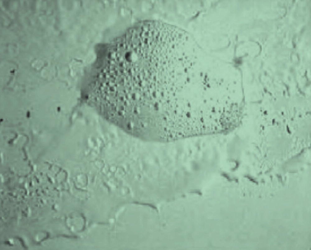
FIGURE 24.24 Microscope image of a typical LLPS.
Source: Reprinted with permission from Derdour [36]. Copyright (2010) Elsevier.
The literature reports that there was an increase in the number of less hydrophilic and less polar drug candidates upon discovery of more potent and improved target‐specific drug molecules [34, 36]. Less hydrophilic molecules have an inherent low polarity with a lack of anchoring sites, and therefore they do not easily self‐assemble in an organized manner. Often, during the early development of drug candidates, seeds of crystalline forms are not available, and creation of first crystals via self‐nucleation is often needed to produce a crystalline solid form. Thus, generating supersaturation is a prerequisite for obtaining a solid form. In early‐stage development, limited data are available regarding the solubility of drug candidates in different solvents. Therefore, supersaturation is usually created by screening methods. Trial and error is also utilized at this stage. However, attempts to crystallize drug substances often lead to a phase separation in which the active molecule is either concentrated in one phase or distributed between many phases.
Two types of oiling out are usually found in the literature [36]:
- Liquid–liquid separation occurs where each phase contains reasonable amounts of solute. This situation can occur when a mixture of solvents is used [37].
- Liquid–liquid separation occurs where one phase contains the solvent(s) and the other phase is mainly formed by the solute in the form of a very heavy viscous oil‐like phase, hence the name oiling out. This phenomenon occurs usually for high solute concentrations at moderately high temperatures.
In all cases, the determination of the phase diagram can help greatly in selecting crystallization conditions to avoid LLPS phenomenon. Once crystalline solids are isolated, oiling out can be avoided via an appropriate seeding strategy [36].
24.6.1.3 Gelation
Molecular gels are defined as 3D assemblies composed of 1D high aspect ratio structures themselves made of non‐covalently linked small organic molecules. Small molecules such those most substances involved in the pharmaceutical industry (except biomolecules) that can form gels are termed low molecular‐mass organic gelators (LMOGs). The 1D assemblies are thought to form due to aggregation of the small molecules upon separation from organic solutions. Because of the high aspect ratio of the 1D assemblies making up the molecular gels, the term “self‐assembled fibrillar networks (SAFINs)” is usually employed to denote them [38].
Due to the non‐covalent nature of the intermolecular interactions involved in SAFINs, these are often thought of as a metastable state that is readily disrupted by applying heat, dilution, shear, or other type of perturbations.
Gels are typically formed via similar phenomena as crystals: an initial aggregation is followed by nucleation, and then the nuclei align to form fibers that ultimately self‐assemble into 3D SAFINs. However, it is still unclear how certain molecules tend to form gels, while others do not [38]. It is currently impossible to predict the propensity of molecule to gelify and the conditions that would favor gel formation. From the crystallization of the pharmaceutical substances perspective, gelation is an undesired phenomenon because of the following reasons:
- Gels are viscoelastic and behave like a fluid, which renders their isolation practically impossible.
- Gels are typically highly viscous and can be “non‐flowing” [39], which results in increased resistance to mixing due to increased viscosity, which can result in equipment failure.
- Because of decreased ordered structure at the molecular level, gelation does not provide the impurity rejection advantage that crystal growth offers [39].
On the other hand, gels were found to be advantageous in providing enhanced means for drug delivery [40, 41] and can be used an additive in crystallization from solution to improve polymorphic selectivity [42].
24.6.1.4 Molecular Rigidity
A common characteristic of organic molecules is their ability to adopt multiple conformations due to their inherent high degree of freedom compared with inorganic substances. In theory, for solution organic chemistry, conformational change always occurs because most organic molecules contain at least one degree of freedom such as a single covalent bond that permits free rotation. Therefore, it is intuitive to expect that in most cases, organic molecules exhibit conformational changes in solution.
There is no consensus about the effect of the existence of several conformers for a given molecule on its crystallizibility, i.e. its propensity to self‐assemble in a new crystalline phase (nucleation). Two general ideas can be extracted from the literature:
- The presence of multiple conformers in solution is expected to increase the barrier to nucleation and decrease the propensity for polymorphism [25]. These authors consider that systems with higher degrees of freedom (i.e. high number of conformers) are expected to be more difficult to nucleate due to lower effective concentration of the conformer that crystallizes, which results in low “effective” supersaturation. Recently, based on ab initio calculations and NMR measurements, it was proposed this behavior is likely to occur if the energy barrier of transition between conformers is higher than approximately 10 kcal/mol [23, 24]. These authors showcased that the presence of rotomers in solution NMR spectra can indicate challenges to nucleation of the species at hand.
- Another school of thought considers that the presence of multiple conformations in solution favors nucleation and polymorphism [26, 28, 31]. It is noted that for most organic compounds, energy difference between different conformers is of the same order of magnitude as the difference in lattice energy between polymorphs (~2 kcal). Therefore, strained conformers, i.e. conformers with higher energy, can crystallize if the resulting crystal lattice provides a better recognition pattern and/or stronger anchoring sites, resulting in low lattice energy.
With respect to crystal growth, two main possibilities are extracted from the literature with regard to the influence of the presence of multiple conformations in solution on crystal growth rate [24]:
- In most cases, the energy barrier to conformational change is relatively low, and forces present on crystal surfaces can readily modify the conformation of the crystallizing species. Thus, it is expected that the presence of multiple conformations in solution does not affect crystal growth kinetics.
- If the energy barrier to conformational change is relatively higher than approximately 10 kcal/mol, the effect of crystal forces on the conformation of the solute is decreased. In this case, crystal growth can be impeded due to one or the combination of the following factors: (i) lower effective supersaturation, (ii) integration site inhibition by conformers that do not crystallize, and (iii) kinetic limitations due to slow equilibration between conformers. The negative effect on crystal growth kinetics is accentuated if the crystallizing species is a high‐energy conformer, i.e. the minor conformer in solution.
Table 24.7 summarizes the expected effect of multiple conformations in solution on propensity for primary nucleation, polymorphism, and crystal growth kinetics based on the energy barrier to conformational conversion.
TABLE 24.7 Expected Effect of Energy Barrier to Conformational Change on Nucleation Polymorphism and Crystal Growth
| ΔE (kcal/mol) | Right Conformer | Nucleation | Polymorphism | Crystal Growth |
| >10 | Minor | Low | Low | Low |
| Major | No effect | Low | No effect | |
| <10 | NA | High | High | No effect |
It is being noted that an increasing number of atropisomers (conformers with half‐life higher than 1000 seconds) are being developed in the pharmaceutical industry due to enhanced activity and target specificity they may offer over more flexible molecules [43–48]. This trend may explain the increasing number of cases of molecular rigidity affecting API crystallization development and form selection [24].
24.6.2 Comprehensive Process Models and Optimization
In recent years, modeling had become increasingly employed in research and development in the pharmaceutical industry. Two main types of modeling can be extracted from the literature:
- Theoretical and semi‐theoretical modeling: The models developed are mainly based on first principles and understanding of the underlying phenomena and mechanisms involved in the processes involved. These models often require some experimental data input to identify kinetic and thermodynamic parameters. Development of theoretical models becomes increasingly challenging with complexity of the mechanisms and phenomena involved in the process (e.g. nonlinearity, large number of phenomena involved, coupling…). Often, these models require adopting some justified hypotheses to simplify the mathematical resolution. Caution should be taken to ensure the models are utilized within the ranges of parameters in which they were validated.
- Empirical or statistical models where models developed are so‐called “black box” models and where the objective is to determine an empirical relationship between outputs and inputs of the model with minimal emphasis of the phenomena and mechanisms involved. These models are usually heavily dependent on experimental data and their accuracy, and predictive power typically improves with the amount of experimental data utilized to build the models. These models have the advantage for removing the mathematical complexity. On the other hand, they present the disadvantage of providing limited improvement of process knowledge.
Modeling is increasingly becoming a core part of research and development of pharmaceutical substances and processes for their manufacture throughout the projects timelines.
24.6.3 Early‐stage Development
Often, in early‐stage development of pharmaceuticals, many drug candidates are transitioned from development. Material availability at this stage is limited, which results in limited experimental data being available and/or obtainable. In addition, because limited data on substance safety and efficacy is available at this stage, it is not justified to invest time and effort to obtain a full and accurate characteristic data set. This peculiarity makes predictive modeling an attractive tool to estimate key parameters that can be indicative of the substance performance and developability. For example, modeling with DFT and Gaussian can inform about molecular flexibility based only on the chemical structure. The results can inform about the crystallizibility of the molecule [24, 49]. Predictive modeling of the solubility based on packages such as NRTL‐SAC and COSMO‐SAC can help design focused experiments to determine accurate solubility data on only selected solvents that can save material and shorten development time. An example of predictive modeling for a marketed drug is shown in Figure 24.25 [50].
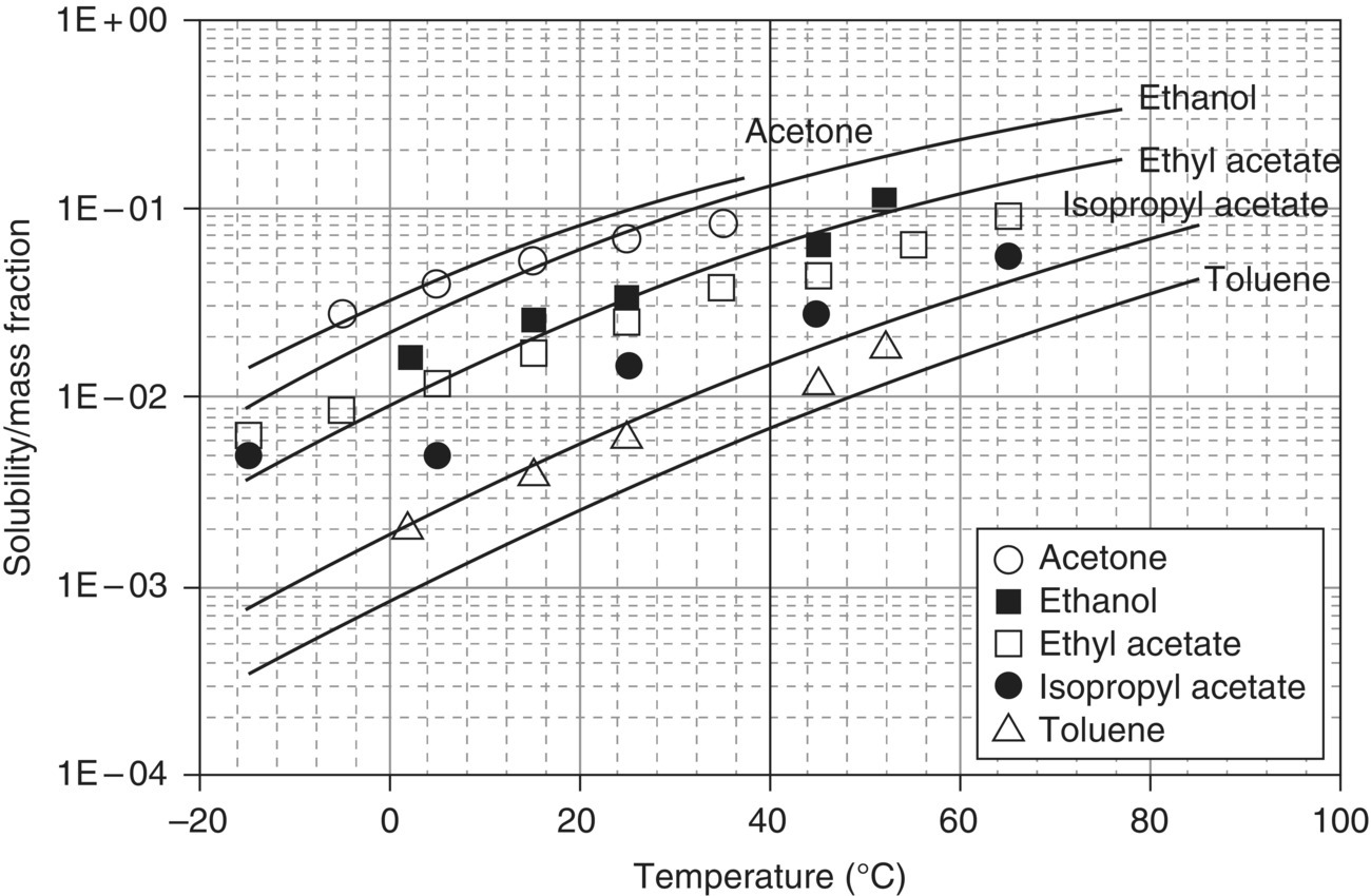
FIGURE 24.25 Predicted and measured solubility of Lovastatin in various solvents as a function of temperature.
Source: Reprinted with permission from Tung et al. [50]. Copyright (2007) Elsevier.
24.6.4 Late‐stage Development
As the program progresses, substance under development can be withdrawn from the project for the following reasons:
- The efficacy of a pharmaceutical substance in achieving its intended physiological response is often demonstrated in earlier‐stage development. That data combined with early proof of safety justify progressing the program through the development life cycle. Initial tests are usually conducted at lowest doses, and during the project progression, dosage is usually increased gradually, and more scrutiny is given to substance safety. The project removes a substance from development if negative data about its safety emerges as dosage increases.
- Often two or more drug substances are progressed in the same program with one molecule being the lead candidate. Withdrawal of one or all contingency molecules can be justified if a substance within the program displays superior efficacy and safety data, minimizing the risk of its failure.
Substances that satisfy efficacy and safety go into late‐stage development. At this stage, larger quantities of the substance are needed to feed various clinical trials, material characterization, and process development efforts. At this stage, a green, efficient, and robust crystallization process is required. Identification of critical process parameters (CPPs) and process knowledge is required. The relationship between CPPs and product attributes must be established in order to establish the design space of the operation, defined as the intervals or ranges of variation of process parameters proven to consistently result in product with quality attributes within specifications. In late‐stage development modeling is becoming increasingly employed and is driven by the following objectives:
- Generate process knowledge and understanding.
- Predict process behavior across and outside the design space.
- Assist with process optimization.
- Minimize experimental work.
24.6.5 Parameter Estimation
In late‐stage development, theoretical and semi‐theoretical modeling are preferred as they generate process knowledge and understanding as opposite to empirical models. Nevertheless, theoretical models still require the knowledge of key kinetic and thermodynamic parameters that are often determined from experiments. In the case of crystallization, several phenomena can occur during the operation. Evidently crystal growth is always present for crystallization to occur, but other phenomena such as nucleation, agglomeration, and breakage can also occur to a certain extent. In addition, these phenomena can have different mechanisms depending on the system at hand and/or the stage of the operation. Often, only one or two phenomena are predominant, which allows for modeling simplification. Hence experiments utilizing process analytical tools (PATs) are typically designed to identify kinetic parameters for main phenomena occurring during the particle‐forming step. Several software packages were developed in recent years to assist scientists and engineers with the estimation of kinetic and thermodynamic parameters that can be utilized in predictive modeling. Such packages are available from companies such as Scale‐up System, ASPEN, and G‐prom. Examples of kinetic parameters estimation for growth‐dominated crystallization can be found in Ma and Wang [51] and Derdour and Chan [52].
24.6.6 Predictive Modeling
Once kinetic and thermodynamic parameters needed to build a model are identified, they are utilized to build predictive models, and the resulting computations are compared with experimental data. This exercise is part of model validation that informs about the predictive power of the model; in other words, how accurate is the model prediction within the process parameters ranges for which it is intended to be valid.
The interval of confidence of computation depends on the criticality of the predicted response. Typically, a high interval of tolerance is required when the predicted response is a CQA.
Once a model to predict a given response is established and validated, it can provide a full landscape for the relationship response/process parameters and be utilized to ascertain the design space and be part of quality by design. In this situation, modeling can also justify the design space and provide confidence about process behavior. Besides chemical and physical quality, manufacturability is an important aspect in drug development. Powder flowability is a required attribute to enable a robust drug manufacturing process. The Carr index is often utilized as a descriptor to assess flowability and is often correlated with the aspect ratio in the case of elongated crystals. An example of predictive modeling of the aspect ratio of an investigational drug is shown in Figure 24.26. In that study [52], predictive modeling was utilized to determine aspect ratio range that would result in an acceptable powder flowability based on the predicted Carr index. In this case, predictive modeling confirmed that the seed loading was the only CPP with respect to the aspect ratio (and powder flowability).
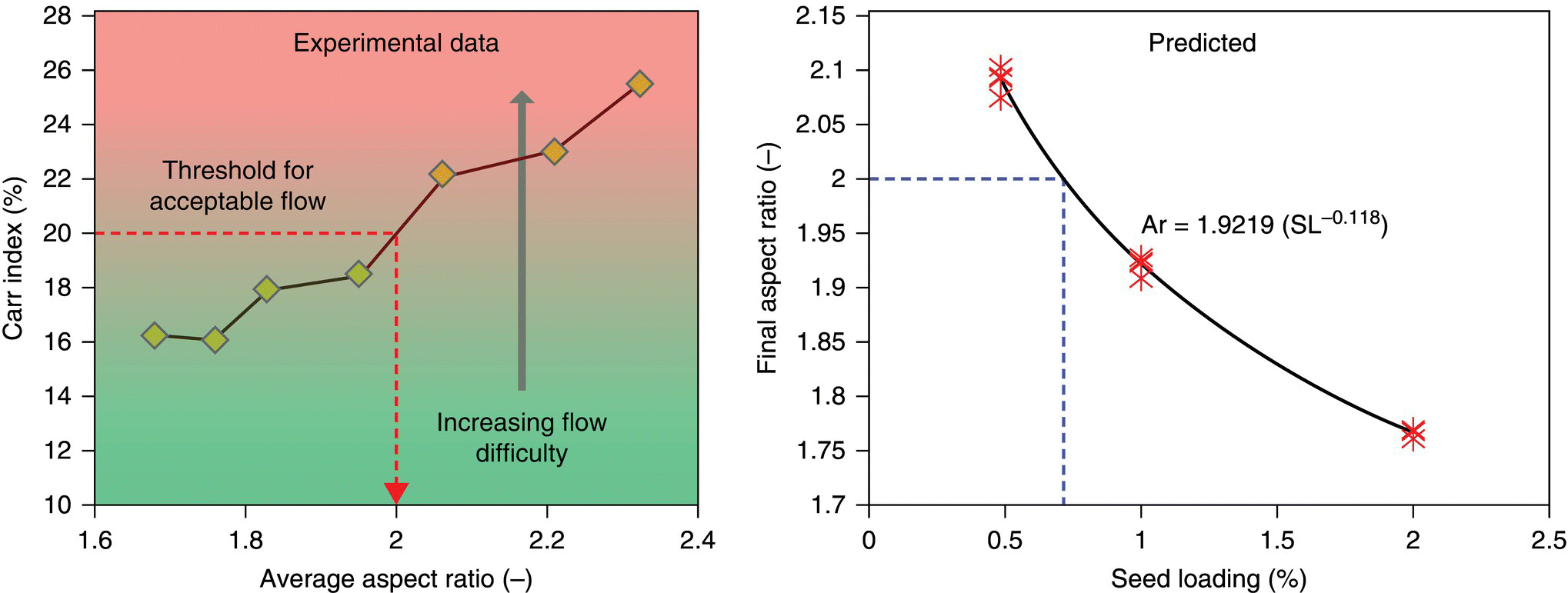
FIGURE 24.26 Predictive modeling of the aspect ratio of an investigational drug (CQA: Ar, aspect ratio: average aspect ratio of crystals [−]; CPP: SL, seed loading [−]).
Source: Reprinted with permission from Derdour and Chan [52]. Copyright (2015) John Wiley & Sons.
24.6.7 Optimization
Another application of modeling is optimization. This exercise is intended to identify operating conditions to attain the following objectives in order of priority:
- Obtain the best product quality.
- Enhance process greenness and robustness.
- Minimize operating costs.
Optimization is typically approached utilizing process parameters at their center point levels. Model predictions of a given response (typically a CQA) are then determined by varying the levels of the inputs (process parameters). The mathematical principle of optimization is usually based on solving first derivative equations for the response where the identified solutions (input parameters) lead to a minimal value of the response.3 In other words, optimization is essentially the resolution of the following equation:
For example, for the case of minimizing the level of an impurity, resolution of the equation above identifies input parameters, Ii, which result in the minimal level of that impurity in the product (response, R). Optimal conditions are identified as the process parameters that result in the best level in terms of quality of the predicted CQA. This exercise can be repeated for other objectives, but it must not be detrimental to product quality (i.e. not deteriorating CQAs levels). For crystallization, particle size distribution can be a CQA, and this is typically controlled by a suitable seeding strategy and supersaturation control. An example of optimized crystallization trajectories for a cooling and antisolvent where the optimized CPP is supersaturation is shown in Figure 24.27 [53].

FIGURE 24.27 Optimized crystallization trajectories for Lovastatin [53].
Source: Reprinted with permission from Nagy et al. [53b]. Copyright (2008) Elsevier.
REFERENCES
- 1. Mullin, J.W. (2001). Crystallization, 4e. Oxford: Elsevier Butterworth‐Heinemann.
- 2. Myerson, A.S. (2002). Handbook of Industrial Crystallization, 2e. Oxford: Butterworth‐Heinemann.
- 3. Tung, H., Paul, E.L., Midler, M., and McCauley, J.A. (2009). Crystallizations of Organic Compounds: An Industrial Perspective. Hoboken: WileyInc.
- 4. Andemichael, Y., Chen, J., Clawson, J.S. et al. (2009). Process development for a novel pleuromutilin‐derived antibiotic. Organic Process Research & Development 13: 729–738.
- 5. Henck, J.‐O. and Kuhnert‐Brandstatter, M. Demonstration of the terms enantiotropy and monotropy in polymorphism research exemplified by flurbiprofen. Journal of Pharmaceutical Sciences 88 (1): 103–108.
- 6. Zaworotko, M.J., Kuduva, S.S., McMahon, J.A. et al. (2003). Crystal engineering of the composition of pharmaceutical phases: multiple‐component crystalline solids involving carbamazepine. Crystal Growth & Design 13 (6): 909–919.
- 7. Childs, S.L., Chyall, L.J., Dunlap, J.T. et al. (2004). Crystal engineering approach to forming cocrystals of amine hydrochlorides with organic acids, molecular complexes of fluoxetine, hydrochloride with benzoic, succini, and fumaric acids. Journal of the American Chemical Society 126 (41): 13335–13342.
- 8. Vogt, F.G., Brum, J., Katrincic, L.M. et al. (2006). Physical, crystallographic, and spectroscopic characterization of a crystalline pharmaceutical hydrate: understanding the role of water. Crystal Growth & Design 6 (10): 2333–2354.
- 9. Gibson, M. (2004). Pharmaceutical Preformulation and Formulation, 1e. Boca Raton, FL: Interpharm/CRC.
- 10. Byrn, S., Pfeiffer, R., Ganey, M. et al. (1995). Pharmaceutical solids: a strategic approach to regulatory considerations. Pharmaceutical Research 12 (7): 945–954.
- 11. Chemburkar, S.R., Bauer, J., Deming, K. et al. (2000). Dealing with the impact of ritonavir polymorphs on the late stages of bulk. Organic Process Research & Development 4: 413–417.
- 12. Santomaso, A., Lazzaro, P., and Canu, P. (2003). Powder flowability and density ratios: the impact of granules packing. Chemical Engineering Science 58 (13): 2857–2874.
- 13. Zhu, H., Yuen, C., and Grant, D.J.W. (1996). Influence of water activity in organic solvent+water mixtures on the nature of the crystallizating drug phase 1‐theophylline. International Journal of Pharmaceuticals 135: 151–160.
- 14. Li, Y., Chow, P.S., Tan, R.B.H., and Black, S.N. (2008). Effect of water activity on the transformation between hydrate and anhydrate carbamazepine. Organic Process Research & Development 12: 264–270.
- 15. Matthews, H.B. and Rawlings, J.B. (1998). Batch crystallization of a photochemical: modeling, control, and filtration. AIChE Journal 44 (5): 1119–1127.
- 16. Larson, M. and Khambaty, S. (1978). Crystal regeneration and growth of small crystals in contact nucleation. Industrial & Engineering Chemistry Fundamentals 17: 160–165.
- 17. Kougoulos, E., Jones, A.G., Jennings, K.H., and Wood‐Kaczmar, M.W. (2005). Use of focused beam reflectance measurement (FBRM) and process video imaging (PVI) in a modified mixed suspension mixed product removal (MSMPR) cooling crystallizer. Journal of Crystal Growth 273 (3–4): 529–534.
- 18. Nocent, M., Bertocchi, L., Espitalier, F. et al. (2001). Definition of a solvent system for spherical crystallization of salbutamol sulfate by quasi‐emulsion solvent diffusion (QESD) method. Journal of Pharmaceutical Sciences 90 (10): 1620–1627.
- 19. Cote, A., Zhou, G., and Stanik, M. (2009). A novel crystallization methodology to ensure isolation of the most stable crystal form. Organic Process Research & Development 13: 1276–1283.
- 20. Dunitz, J.D. and Bernstein, J. (1995). Disappearing polymorphs. Accounts Chemical Research 28: 193–200.
- 21. Bernstein, J., Davey, R.J., and Henck, J.O. (1999). Concomitant polymorphs. Angewandte Chemie International Edition 38: 3441–3461.
- 22. Grant, D.J.W. (1999). Theory and origin of polymorphism. In: Polymorphism in Pharmaceutical Solids (ed. H.G. Brittain), 1–33. New York: Marcel Dekker.
- 23. Derdour, L., Pack, S.K., Skliar, D. et al. (2011). Crystallization from solutions containing multiple conformers: a new modeling approach for solubility and supersaturation. Chemical Engineering Science 66: 88–102.
- 24. Derdour, L. and Skliar, D. (2014). A review of the effect of multiple conformers on crystallization from solution and strategies for crystallizing slow inter‐converting conformers. Chemical Engineering Science 106: 275–292.
- 25. Yu, L., Reutzel‐Edens, S.M., and Mitchell, C.A. (2000). Crystallization and polymorphism of conformationally flexible molecules: problems, patterns and strategies. Organic Process Research & Development 4: 396–402.
- 26. Buttar, D., Charlton, M.H., Docherty, R., and Starbuck, J. (1998). Theoretical investigations of conformational aspects of polymorphism. Part 1: o‐acetamidobenzamide. Journal of the Chemical Society, Perkin Transactions 2: 763–772.
- 27. Yu, L. (2002). Color changes caused by conformational polymorphism: optical‐crystallography, single‐crystal spectroscopy, and computational chemistry. Journal of Physical Chemistry A 106: 544–550.
- 28. Nangia, A. (2008). Conformational polymorphism in organic molecules. Accounts of Chemical Research 41: 595–604.
- 29. Arora, K.K. and Zaworotko, M.J. (2009). Pharmaceutical co‐crystals: a new opportunity in pharmaceutical science for a long‐known but little‐studied class of compounds. In: Polymorphism in Pharmaceutical Solids, 2e (ed. H.G. Brittain), 282–317. New York: Informa Healthcare.
- 30. Morissette, S.L., Almarsson, Ö., Peterson, M.L. et al. (2004). High‐throughput crystallization: polymorphs, salts, co‐crystals and solvates of pharmaceutical solids. Advanced Drug Delivery Reviews 56: 275–300.
- 31. Starbuck, S., Docherty, R., Charlton, M.H., and Butter, D. (1999). A theoretical investigation of conformational aspects of polymorphism. Part 2. Diarylamines. Journal of the Chemical Society, Perkin Transactions 2: 677–691.
- 32. Brittain, H.G. (1999). Application of the phase rule to the characterization of polymorphic systems. In: Polymorphism in Pharmaceutical Solids, 35–72. New York: Marcel Dekker.
- 33. Derdour, L., Reckamp, J.M., and Pink, C. (2017). Development of a reactive slurry salt crystallization to improve solid properties and process performance and scalability. Chemical Engineering Research & Design 121: 207–218.
- 34. Serajudin, A.T.M. and Pudipeddi, M. (2002). Salt selection strategies. In: Handbook of Pharmaceutical Salts: Properties, Selection and Use (ed. P.H. Stahl and C.G. Wermuth), 147–172. Zürich: Verlag Helvetica Chimica Acta.
- 35. Maeda, K., Nomura, Y., Fukui, K., and Hirota, S. (1997). Separation of fatty acids by crystallization using two liquid phases. Korean Journal of Chemistry 14: 175–178.
- 36. Derdour, L. (2010). A method to crystallize substances that oil out. Chemical Engineering Research & Design 88: 1174–1181.
- 37. Veesler, L., Lafferrère, L., Garcia, E., and Hoff, C. (2003). Phase transitions in supersaturated drug solution. Organic Process Research & Development 7: 983–989.
- 38. Caran, K.L., Lee, D.C., and Weiss, R.G. (2013). Molecular gels and their fibrillar networks. In: Applications, Soft Fibrillar Materials: Fabrication and Use (ed. X.Y. Liu and J.L. Li), 1–75. Weinheim: Wiley‐VCH.
- 39. Yin, Y., Gao, Z., Bao, Y. et al. (2014). Gelation phenomenon during antisolvent crystallization of cefotaxime sodium. Industrial & Engineering Chemistry Research 53: 1286–1292.
- 40. Langer, R. (2000). Biomaterials in drug delivery and tissue engineering: one laboratory’s experience. Accounts of Chemical Research 33: 94–101.
- 41. Xing, B., Yu, C.W., Chow, K.H. et al. (2002). Hydrophobic interaction and hydrogen bonding cooperatively confer a vancomycin hydrogel: a potential candidate for biomaterials. Journal of the American Chemical Society 124: 14846–14847.
- 42. Diao, Y., Whaley, K.E., Helgeson, M.E. et al. (2012). Gel‐induced selective crystallization of polymorphs. Journal of the American Chemical Society 134: 673–684.
- 43. Laplante, S.E., Fader, L.D., Fandrick, K.R. et al. (2011). Assessing atropisomer axial chirality in drug discovery and development. Journal of Medicinal Chemistry 54: 7005–7022.
- 44. Laplante, S.E., Edwards, P.J., Fader, L.D. et al. (2011). Revealing atropisomer axial chirality in drug discovery. ChemMedChem 6: 505–513.
- 45. Bringmann, G., Price Mortimer, A.J., Keller, P.A. et al. (2005). Atroposelective synthesis of axially chiral biaryl compounds. Angewandte Chemie International Edition 44: 5384–5427.
- 46. Zhou, Y.S., Tay, L.K., Hughes, D., and Donahue, S. (2004). Simulation of the impact of atropisomer interconversion of plasma exposure of atropisomers of an endothelin receptor antagonist. The Journal of Clinical Pharmacology 44: 680–688.
- 47. Albert, J.S., Ohnmacht, C., Bernstein, P.R. et al. (2004). Structural analysis and optimization of NK1 receptor antagonists through modulation of atropisomer interconversion properties. Journal of Medicinal Chemistry 47: 519–529.
- 48. Fukuyama, Y. and Asakawa, Y. (1991). Novel neurotrophic isocuparane‐type sesquiterpene dimers, mastigophorenes A, B, C and D, isolated from the liverwort mastigophora didados. Journal of the Chemical Society, Perkin Transactions 1 (11): 2737–2741.
- 49. Price, S.L. (2013). Why don't we find more polymorphs? Acta Crystallographica Section B: Structural Science Crystal Engineering and Materials 69: 313–328.
- 50. Tung, H.H., Tabora, J., Variankaval, N. et al. (2008). Prediction of pharmaceutical solubility via NRTL‐SAC and COSMO‐SAC. Journal of Pharmaceutical Sciences 97: 1813–1820.
- 51. Ma, C.Y. and Wang, X.Z. (2012). Model identification of crystal facet growth kinetics in morphological population balance modeling of L‐glutamic acid crystallization and experimental validation. Chemical Engineering Science 70: 22–30.
- 52. Derdour, L. and Chan, E.J. (2015). A model for supersaturation and aspect ratio for growth dominated crystallization from solution. The AIChE Journal 61: 4456–4469.
- 53. (a) Nagy, Z.K., Fujiwara, M., and Braatz, R.D. (2007). Recent advances in the modelling and control of cooling and antisolvent crystallization of pharmaceuticals. Proceedings of the 8th IFAC Symposium on Dynamics and Control of Process Systems, Cancún, Mexico (4–8 June 2007), Vol. 2, pp. 29–38. (b) Nagy, Z.K., Fujiwara, M., and Braatz, R.D. (2008). Modelling and control of combined cooling and antisolvent crystallization processes. Journal of Process Control 18 (9): 856–864.