
8
REACTION KINETICS AND CHARACTERIZATION
Utpal K. Singh, Brandon J. Reizman, Shujauddin M. Changi, and Justin L. Burt
Eli Lilly and Company, Indianapolis, IN, USA
Chuck Orella
Merck & Co., Inc., Rahway, NJ, USA
8.1 INTRODUCTION
The ability to effectively characterize and interpret reaction kinetic data is of fundamental importance for chemical development. In the pharmaceutical industry, reaction kinetics factor prominently in the areas of process optimization, process safety evaluation, understanding of scale sensitivity, and assessment of process robustness. Beyond these specific applications, the role that reaction kinetic understanding can have at all stages of process development is difficult to overstate. Examples in which detailed kinetic understanding can impact the viability of a process include instances:
- Where mechanistic insights are exploited in the mitigation of a key impurity, degradant, or other process failure mode.
- Where a successful process scale‐up is contingent upon understanding the competition between kinetic and mass transfer effects.
- Where online measurements enable process adjustments for safer operation, improved product quality, or increased yield.
- Or where a reaction pathway model is leveraged to direct experimental work.
Above all else, the investigation of reaction kinetics affords scientists and engineers a means to quantifiably impact a chemical system throughout development from the molecular scale to commercial‐scale manufacturing.
The literature has many excellent texts and articles devoted to a variety of perspectives on chemical reaction engineering and kinetics. Generally, these fall into the categories of mechanistic chemistry, reaction kinetics, and reactor design and operation. We encourage readers to sample texts from all of these perspectives [1–6]. In this chapter, we focus on those aspects of reaction characterization and scale‐up that are of greater relevance to chemists and engineers working in the pharmaceutical industry and highlight those methods that have the potential to significantly improve the efficiency and effectiveness of development activities.
Two aspects in particular have historically made pharmaceutical processing unique from commodity and (to a lesser degree) specialty chemicals. The first differentiating feature is the complexity and richness of the chemistry, with multiple reactive moieties present in molecules available for desired and, often, undesired reaction pathways. Second, while bulk chemical manufacturers have embraced continuous processing as a means of enabling smaller process footprints and more sophisticated engineering controls, pharmaceutical processing has mostly remained steadfast in carrying out sequential batch operations in stirred tank reactors. Transitioning away from this batch mindset requires increased integration of process chemistry and chemical engineering in the design of continuous manufacturing processes for pharmaceuticals, a compelling area of development that will be referenced in examples throughout this chapter.
The diversity in chemistry practiced in the pharmaceutical industry can be viewed from two competing perspectives. From a molecule‐to‐molecule standpoint, each chemical synthesis brings new challenges, ranging from transformations that disobey accepted heuristics, to the control of competing impurities and degradants, to difficult‐to‐quantify mass transfer effects. To address this complexity, it is necessary to design and execute the proper experiments that help uncover the underlying mechanisms, reaction pathways, and rates. The application of kinetic models in describing each of these phenomena offers a quantitative approach that can help with testing mechanistic hypotheses or with transitioning to a new target reaction condition or processing scale.
From a macroscopic perspective, although active pharmaceutical ingredients vary greatly in structure and function, the variety of chemical transformations employed by pharmaceutical chemists to construct molecules is hardly as diverse as the molecules themselves. For example, a survey of the most commonly employed chemical transformations at companies such as GlaxoSmithKline (GSK), AstraZeneca, and Pfizer revealed that more than 80% of developed reactions can be categorized into one of eight different classes: heteroatom alkylations and arylations, acylations, C─C bond formations, aromatic heterocycle formations, deprotections, protections, reductions, and oxidations [7]. The majority of the remaining reactions were functional group interconversions or additions. Efforts to minimize the time and labor involved in process development should begin with standardizing the knowledge of mechanistic and scale‐dependent factors encountered in each of these common reaction classes.
In addition to mechanistic insight, characterization of reaction kinetics requires an understanding of the interplay between the rate of chemical transformation and the physics of the system. Scale sensitivity is exhibited when the rate of a physical transformation (i.e. rate of mixing, heat input, or heat removal) becomes nearly equal to or slower than the rate of chemical transformation. A different study of the pharmaceutical industry surveyed 22 different processes and classified the 86 reactions used in those processes according to overall kinetics and the physical nature of the reaction mixture [8]. Nearly 75% of the reactions were classified as having a potential for scale sensitivity. A vast majority of the surveyed reactions were heterogeneous. The combination of the multiphasic nature of the reaction mixture with the intrinsic speed of the reaction results in the potential for scale sensitivity. This chapter will present some of the techniques for quantitative assessment when there is a scale‐dependent competition between the rates of chemical transformation and physical transformation, i.e. limitations due to the rates of mass and heat transfer.
A unique historical aspect of the pharmaceutical industry has been the use of batch processing for the majority of operations. The demand placed on the development scientist has then been the scale‐up of reactions from the milliliter scale to the cubic meter scale (6 orders of magnitude). Over such a wide range of scale, changes in the observed reaction behavior owing to the competition between reaction rate and mass transfer are often observed. Such changes can lead to suboptimal cycle time, or even compromised product quality upon scale‐up for manufacturing if not managed appropriately. To successfully scale-up, it is necessary to take both kinetic and equipment design considerations into account such that the perceived rate‐limiting step is understood at every scale.
Pharmaceutical companies have begun to leverage the operation of chemical reactions in continuous mode to decrease the overall magnitude of scale‐up, thus lessening the severity of scale sensitivity observed upon manufacturing [9–11]. The ratio of surface area to volume is generally much greater for continuous reactors than for industrial batch reactors. This affords heat and mass transfer rates that are more consistent with laboratory‐scale experiments. Classical examples of continuous reactors offering an advantage over batch operating conditions involve fast reactions that risk “overreaction” of the desired product [5] or cases where safety is enhanced by decreasing the total amount of material in the reactor at a given time. Examples of safety enhancement in continuous reactors include cases where there is a risk of thermal runaway (e.g. Grignard reactions, lithiations, or nitrations) or where hazardous reagents are employed (e.g. syntheses involving azides, peroxides, strong reductants, or reactive gases such as hydrogen, oxygen, fluorine, or chlorine). For the purpose of the ensuing discussion, it is important to emphasize that in the absence of mixing or thermal effects, the fundamental kinetic data obtained from a plug flow continuous reactor will be identical to the kinetics measured in a stirred tank batch reactor [5]. Continuous processing also creates opportunities for more in‐line and at‐line kinetic measurements, as will be discussed later in this chapter, and can lead to higher plant productivity than a comparable batch operation [12]. A few of the advantages that continuous reactors offer in comparison with traditional batch processing are summarized in Table 8.1.
TABLE 8.1 Advantages of Continuous Reactors in Comparison to Batch Reactors
| Characteristic | Batch (8000 L Stirred Vessel) | Continuous (1 in pipe reactor) | Advantage |
| Mixing time | >10 s (bulk blending) | >0.1 s | Rapid blending of reagents for fast reactions |
| Surface to volume available for heat transfer | ~2 m−1 | ~200 m−1 | Superior temperature uniformity with fewer “hot spots” |
| Typical temperature and pressure limit (in the absence of special reactor designs) | 150 °C 10 bar |
200–250 °C 30–150 bar |
Ease of running reactions above the normal boiling point of solvents. Higher concentrations of gaseous reagents dissolved |
| Instantaneous amount reacting | 100–1000 kg | 1–5 kg | Lower energy potential and impact of runaway reaction |
This chapter is divided into four sections. We begin by reviewing the common factors contributing to observed reaction kinetic behavior: kinetic effects, mass transfer effects, thermal (energy‐related) effects, and dispersion. Subsequent sections discuss strategies for the characterization of reaction behavior in the presence of these different phenomena and lay the framework for transforming the data collected from these characterization experiments into a kinetic model. Both empirical and mechanistically based approaches are highlighted. Finally, we discuss some of the more recent developments in the field and the impact that new methodologies are having both in the laboratory and in the manufacturing environment. A number of academic and industrial examples are provided throughout the chapter to illustrate the implementation of the discussed techniques. We hope the reader will come to appreciate the complexity of problems solvable using these characterization and numerical tools in concert with an applied understanding of the competition between reaction kinetic and physical phenomena.
8.2 FUNDAMENTALS OF CHEMICAL REACTION KINETICS
Fundamental understanding of the relevant rates of reactions is crucial in order to optimize process performance criteria such as yield and selectivity and to build quantitative relationships between input attributes, process parameters, and the desired outcomes of a reaction. Reactive chemical systems can be divided into two classes: homogeneous reactions, involving only a single phase, or heterogeneous reactions, involving two or more phases (e.g. solid–liquid, liquid–liquid, gas–liquid, or gas–solid–liquid). A small subset of homogenous reactions are elementary, i.e. these reactions occur in a single step with a rate that scales proportionally with the concentrations of the species in the reaction. The majority of reactions comprise multiple steps occurring in series or parallel [4, 13], passing through both detectable and undetectable intermediates to ultimately afford the desired product and (undesired) reaction impurities. In general, a robust process chemistry and reproducible reaction performance require an understanding of the competing rates of reactions, together with mixing, mass transfer, distribution among phases, and heat transfer considerations. This section provides considerations for determining the rates of reaction and mixing for various categories of reactions encountered in pharmaceutical processes. Understanding of these rates can then be used in conjunction with the physics and energetics of the system to select the most appropriate reactor type and mode of operation.
8.2.1 Reaction Rate and Mass Balance
For a reactive single‐phase system,
there exists a reaction time scale defined by the kinetics and independent of mass transfer limits (e.g. mixing, diffusion). The reaction rate (rA) for disappearance of moles of limiting reactant A (NA) can be written in a differential form as shown in Eq. (8.1), with V being the overall volume of the system:
The rates of reaction for each component (ri) are interrelated based on the mass balance for the system, as shown in Eq. (8.2):
The rate of a chemical reaction is generally determined empirically as a function of the concentration of reactive species and the temperature. In a limited number of cases, the reaction is elementary in that no reactive intermediate is formed in the transition from reactants to products. For elementary reactions, the reaction rate is then exactly proportional to the concentrations of reacting species. Many reacting systems, however, consist of a sequence of mechanistic steps (in series, in parallel, or both) proceeding at unique rates that in combination afford an observed rate law. Depending upon the relative rates of the mechanistic steps, the measured rate law may still simplify to a power law along the lines of Eq. (8.3):
where
- k is the reaction rate constant.
- Ci are concentrations of the ith species.
- α, β are the reaction orders.
A rate law may even simplify to the same expression that would be obtained was the reaction assumed to be elementary (α = β = 1 in Eq. (8.3)). Methods are discussed in this chapter for testing whether a sequence of proposed elementary or nonelementary reactions consistently describes the experimental data.
Though not a universal statement, reaction kinetics that do not adhere to a simple power law often indicate the presence of competing processes within the reaction system. Examples of such behavior may be the result of a reversible or inhibitory reaction involving one or more of the products, a reaction cycle in which a reactive species or catalyst must be regenerated in order for the reaction to proceed, or chemistry involving multiple phases where the overall rate is dependent on the intrinsic reaction rate and the rate at which the species can transition between phases. This last example is of particular emphasis in this chapter, as the rate of mass transfer of reagents between phases is a contribution that often appears only when examining the chemistry across different scales. In light of this, it is important to keep in mind that the converse of this paragraph's opening sentence should not be assumed, i.e. reaction kinetics that adhere to a simple power law do not necessarily imply simplicity of the underlying chemical system. Several examples showing a change in apparent kinetics with reaction conditions and/or process scale can be found throughout this chapter.
8.2.2 Kinetic Considerations
The act of measuring a rate law – power law or otherwise – is a simple activity in comparison with the act of interpreting kinetic results with the goal of optimizing for yield or selectivity, scaling up a process, or understanding the reaction mechanism. When embarking on any of these tasks, it is important to have awareness of all factors that may contribute to the observed reaction rate, including contributions from the reaction medium (solvent), mass transfer, and heat transfer. Above all else, it is of utmost importance to have an understanding of the factors that govern the reaction itself.
In addition to the concentration of species, the rates of elementary reaction steps are governed by a rate constant, assumed to be of the Arrhenius form
where
- A is the pre‐exponential factor.
- EA is the activation energy.
- R is the gas constant.
- T is the temperature.
Whereas A and EA are commonly found in practice by regression to experimental data (see Section 8.4), quantum mechanical tools can in principle be used for the estimation of both parameters in an effort to confirm mechanistic hypotheses or to predict reactivity [6, 14]. A physical interpretation of A and EA applicable to many reactive systems can be extracted from transition state theory, which postulates that reactants must traverse a barrier of higher‐energy states before conversion to products. At the minimum height of this barrier is the transition state, which resides in energy above the starting reactants at a difference equal to the activation energy, EA. The pre‐exponential factor, A, reflects the number of degrees of freedom available at that transition state; a lesser value of A indicates a more constrained transition state and would imply a lower probability of proper alignment of the reactant orbitals for a reaction to occur.
In the simplest terms, the art of designing chemical reactions to be faster or more selective reduces to the identification of reagents or methods that impact either or both of the coefficients in Eq. (8.4). Most notably, catalysts are employed to reduce the height of the activation energy barrier. Transition metal catalysts are prevalent throughout chemical processing because of their ability to adopt different oxidation states in support of what would otherwise be much more energetically unfavorable intermediates. For reactions directed at a particular site of a molecule, heterogeneous reactions occurring at the surface of a catalyst can also constrain reactive species such that a targeted transition state becomes more favorable. Among the attributes of the reactants themselves that contribute to the reaction rate are the electronics of the molecules, i.e. the ability to donate or withdraw charge and hence minimize the energy burden of a transition state, and steric factors that impact the ability of the molecules to conform to the proper orientation for the reaction to occur. The reaction medium (solvent) has the potential to significantly impact both of these attributes.
The solvent in which solution‐phase chemistry occurs can impact the rate, selectivity, and mechanism of the desired reaction [15]. Factors impacting solvent selection include compatibility with the mechanism of the proposed reaction, the ability to dissolve substrate, reagent, and/or product at minimal dilution, physical compatibility with the intended process conditions (e.g. reaction temperatures above the freezing point and below the boiling point of the solvent), occupational health, process safety, and environmental considerations, as well as solvent cost and commercial availability. In practice, solvent selection is often driven by empirical knowledge of solvents that have worked in the past for a given type of reaction, derived from institutional history, accumulated literature, or personal experience.
An industrial example of solvent selection impacting reaction selectivity was reported by researchers at Eli Lilly [16]. Referring to Scheme 8.1, hydroxide‐catalyzed conversion of nitrile 1 to the desired amide 2 was susceptible to over‐hydrolysis, affording a carboxylic acid impurity 3. N‐Methyl‐2‐pyrrolidone (NMP) was identified as a solvent that, in addition to affording favorable solubility properties, exhibited a rate of hydrolysis comparable with the amide. Sacrificial hydrolysis of NMP to 4‐(methylamino)butyric acid 4 consumed excess hydroxide, protecting the amide and limiting formation of the carboxylic acid impurity.
SCHEME 8.1 Hydroxide‐catalyzed hydrolysis of 1 in the presence of NMP.
A kinetic model was developed based on the elementary reactions:

Kinetic parameters were regressed, and the resultant kinetic model was employed to probe the robustness of the process chemistry in silico. Figure 8.1 illustrates the enhanced process robustness realized by employing NMP as a sacrificial solvent. The design requirements were less than 0.3% residual nitrile and less than 2.5% carboxylic acid impurity at the reaction endpoint. Referring to the dashed reaction profiles in Figure 8.1, in the absence of NMP hydrolysis, there was only an approximately 30 minute window (from 90 to 120 minutes) in which to stop the reaction while satisfying both design requirements. With the sacrificial hydrolysis of NMP (Figure 8.1, solid reaction profiles), the design requirement of less than 0.3% residual substrate was satisfied after 3 hours of reaction, and the level of 3 remained within its target range of less than 2.5% for several hours, affording a robust window in which to stop the reaction. The acceptable time intervals for reaction control without (shorter duration) and with (longer duration) NMP are included for comparison in Figure 8.1.

FIGURE 8.1 Model‐predicted reaction profiles with and without use of NMP as a sacrificial solvent, assessed at target reaction conditions (75 °C and 0.25 equiv. NaOH).
Source: Reprinted with permission from Niemeier et al. [16]. Copyright 2014, American Chemical Society.
8.2.3 Mass Transfer Considerations
An understanding of mixing rates is important to the characterization and scale‐up of heterogeneous reactions. Mass transfer‐limited processes can give an erroneous sense of kinetics when scaled up, impacting the desired outcome. Detailed reviews can be found in literature that describe mixing dynamics at molecular and larger scales [17, 18].
The Damköhler number can be used to assess the effect of scale on reaction kinetics:
Here, the rate of physical processes can include any rate of mixing, including those associated with mass transfer such as liquid–liquid mixing, gas absorption, gas desorption, and solid suspension. In general, no scale sensitivities would be expected when the rate of the chemical transformation is slower than that of the relevant physical process. In contrast, scale sensitivities are observed when the rate of the physical process is slower than the rate of the chemical transformation. This statement holds not only for the desired reaction pathway but also for other chemical pathways that may result in impurity formation.
The rate of chemical transformation generally takes the form of Eq. (8.1). The rate of mass transfer is expressed generally as a function of the mass transfer coefficient (ksas) and the difference in concentration of a given species between the two phases:
Numerous correlations have been reported in the literature describing functional relationships between the nondimensional groups of Reynolds number (Re), Schmidt number (Sc), and Sherwood number (Sh). These dimensionless parameters are defined by Eqs. (8.7)–(8.9):
where
- ρ = the fluid density
- u = the velocity
- μ = the fluid viscosity
- Dm = the diffusion coefficient
- d = characteristic linear length traveled by the fluid
The characteristic length d is system‐dependent and may represent an average particle diameter, the diameter of an impeller, or a pipe diameter, depending on the application. In general, these correlations have the functional form
where the constants x, y, and z vary depending on the system under consideration. While it is difficult to make broad generalizations regarding how to measure competing reaction kinetic and mass transfer effects over a diverse range of chemical environments, generalizations can be made for specific physical processes. To that extent, relevant mass transfer regimes will be discussed as follows.
8.2.3.1 Solid–Liquid Transfer
Many industrial applications involve insoluble reagents, catalysts, or intermediates. In these cases, solid–liquid transfer effects need to be characterized and understood, but the deconvolution of mass transfer rates from reaction kinetics may be complex. A number of different mass transfer correlations for solid–liquid systems are available in the literature [19]. One issue that arises when utilizing correlations in the form of Eq. (8.10) is the formulation of the Reynolds number. A number of different modified particle Reynolds number expressions are presented in the literature [20]. Many studies have been published on the mass transfer to particles in both stirred tanks and pipes [21–27]. It should be noted that a variety of substrates (e.g. lead sulfate, barium sulfate, silver chloride) have been used for dissolution measurements, with some systems being especially susceptible to agglomeration and/or subjected to additional surface resistances. There is always some uncertainty when applying these correlations to a new system.
Understanding the limitations of correlations, it is often preferable to explicitly measure the mass transfer constant across the solid–liquid interface using dissolution measurements [28]. This approach allows a direct measurement of the mass transfer rate constant for comparison with the corresponding reaction rate constant. Alternatively, one could combine the rate constant for solid–liquid transfer with the intrinsic reaction rate constant and then use the relative activation energies as a means to deconvolute mass transfer and reaction‐limited regimes. For a first‐order reaction with rate constant kr, the rate expression that combines the reaction rate and the rate of mass transfer can be written as Eq. (8.11) [29, 30]:
where ksas is the rate constants for mass transfer across the solid–liquid interface. In cases where the mass transfer across the solid‐to‐liquid interface is rapid (ksas ≫ kr), the rate expression simplifies to ri = krCi, and chemical kinetics are rate controlling. In cases where the mass transfer across the solid–liquid interface is slow (ksas ≪ kr), the rate expression simplifies to ri = ksasCi, and mass transfer across the boundary layer is the rate‐limiting step.
The temperature dependence of the rate constant kr and ksas allows for deconvolution of the chemical kinetics from the mass transfer kinetics. The influence of temperature on the mass transfer rate is primarily through its influence on viscosity and/or diffusion coefficients. There is only a modest effect of temperature on these variables, and as a result, the mass transfer rates typically exhibit a weak dependence with temperature. As a general heuristic, activation energies for mass transfer‐limited processes are typically on the order of 10–20 kJ/mol, compared with 40–60 kJ/mol for reaction‐limited processes [31].
Calculations to estimate the transport from particles in heterogeneous reactions have been outlined by Zwietering [32]. These mass transfer rates are influenced by agitation speed, up to a certain point (called the just‐suspended speed) beyond which the particles no longer form a layer at the bottom of the vessel. Experimental data and mathematical correlations indicate that the rate of mass transfer in solid–liquid systems changes appreciably up to the just‐suspended speed for particles. Further increases in mixing intensity once solids have already been suspended give only marginal increases in mass transfer [20]. Changi and Wong illustrate one such example using a Grignard reaction that accounts for mass transfer effects and the corresponding intrinsic kinetic rate constant [33]. Although the presented model does not capture the actual mechanism for Grignard reagent formation and is purely phenomenological, it is able to capture the physical and chemical aspects of the process across various scales by using the Zwietering criterion to estimate the just‐suspended speed for the particles.
8.2.3.2 Liquid–Liquid Transfer
There have been several reviews documenting the effect of liquid–liquid mixing in pharmaceutical applications [34]. Among the powerful tools in characterizing liquid–liquid mixing are Bourne reactions; these are pairs of competing reactions designed such that the selectivity toward a slower‐forming by‐product is characteristic of the rate of mixing. The known rate constants of the Bourne reaction can be used to quantify mixing times and thus understand the interplay of mixing and chemical kinetics. Prudhomme and Johnson [35], Mahajan and Kirwan [36], and Singh and coworkers [37] have used such reaction systems to characterize different mixing geometries to enhance mixing efficiency and reduce mixing times.
For miscible liquid–liquid systems, the impact of mixing can be determined by conducting one of a number of diagnostic tests, depending on the reaction kinetics and the mode of mixing: micromixing or macromixing. Micromixing is associated with molecular diffusion and stretching of the fluid under small‐length‐scale laminar flow conditions, under which viscous forces dominate over inertial forces. Macromixing occurs in conventional batch or continuous stirred tank reactors due to mechanical agitation. This is typically in the turbulent regime. Correlations for mixing times for macromixing and micromixing regimes have been articulated in the literature [38]. Use of the Damköhler number offers guidance on determining the effect of mixing on reaction performance.
In lieu of correlations, the impact of the order of addition upon reaction performance is a simple metric for assessing mixing‐limited regimes. Consider a case of parallel reactions, in which a stream of A is added to a vessel containing B to yield product C and an impurity D.
If the reaction is conducted in the reverse order of addition, i.e. a stream of B is added to a vessel containing A and no effect on rate of impurity formation is observed, then it can be concluded that mixing effects are negligible. This is because the two addition modes mimic conditions of highly segregated concentrations of either A or B. In contrast, if the order in B for formation of species C is greater than that for formation of D, then the two addition modes would afford different ratios of species C and D, hence mixing sensitivity could be pronounced upon scale‐up.
There are several ways to manage mixing sensitivity. For example, static mixers or auxiliary mixing devices such as mixing elbows or vortex mixers can be used to enhance mixing while leaving the reaction kinetics unaffected. Alternatively, the reaction kinetics can be modified by leveraging differences in reaction rates between the different chemical pathways. This may involve running the reaction at a different concentration (to exploit differences in reaction order) or at a different temperature (to exploit differences in activation energy).
8.2.3.3 Gas–Liquid Transfer
Gas–liquid mixing plays a central role in a number of commercialized synthetic processes. Transport of gas into and out of solutions can drive reaction rates and selectivity. A procedure for measuring the rate of mass transfer from the gas to liquid phases has been detailed previously [39]. The integral approach for measuring the vapor–liquid mass transfer coefficient kLa is shown in Eq. (8.12):
where
- Po is the solvent vapor pressure.
- Pf is the final system pressure.
- Pi is the initial system pressure.
- P(t) is the system pressure measured during the course of the experiment.
Plotting the left‐hand side of Eq. (8.12) versus time yields a slope with units of 1/time and represents the mass transfer constant from gas phase to liquid phase. Alternatively, the initial slope of the pressure drop at the start of an uptake experiment to estimate the value of kLa is given by Eq. (8.13):
For both large‐ and small‐scale measurements, it is important to understand the ramp‐up time for an agitator to reach full power. Experimental details for measuring kLa and factors that affect gas–liquid mixing efficiency have been captured elsewhere [40].
As in the case of solid–liquid and liquid–liquid systems, the convolution of reaction rate with mass transfer from gas phase to liquid phase can be described using the Damköhler number:
where
- rrxn is the intrinsic reaction rate.
-
 is the maximum rate of transfer from the gas phase to the liquid phase.
A ratio of Da > 1 is indicative of mass transfer limitations whereas Da < 0.1 is indicative of a regime free of mass transport limitations. An example of the utility of the Damköhler number arises for debenzylation of a fumurate salt of an amine to give the corresponding succinate salt of the secondary amine (see Scheme 8.2). The hydrogenation process initially involves reduction of the fumaric acid to succinic acid followed by debenzylation to form the corresponding secondary amine succinate salt. The reaction rate profile as a function of hydrogen pressure is shown in Figure 8.2. The results indicate a positive‐order dependence of the rate of fumaric acid reduction on hydrogen pressure compared with zero‐order dependence for debenzylation. Hydrogen starvation resulted in significant decrease in the rate of fumaric acid reduction with little or no effect on the rate of debenzylation, resulting in the accumulation of the fumaric acid in the presence of a secondary amine, thereby increasing the propensity for the formation of the Michael adduct 7 (Scheme 8.3).
SCHEME 8.2 Debenzylation and corresponding fumaric acid reduction.

FIGURE 8.2 Rate profile for concomitant debenzylation and fumaric acid reduction over Pd/C for reaction in Scheme 8.2.

SCHEME 8.3 Michael adduct formation reaction.
The Damköhler number for this process is defined by Eq. (8.15):
When Da < 1, the rate of hydrogen transfer from the gas phase to liquid phase is rapid compared with fumaric acid reduction, and as a result the hydrogenation proceeds rapidly. When Da > 1, the rate of hydrogen transfer is slower than the rate for fumaric acid reduction; as a result, the rate of fumaric acid reduction is slowed to the point that subsequent debenzylation can occur simultaneously, thereby allowing the deprotected secondary amine to react with the fumaric acid to form the Michael adduct.
In considering gas–liquid reactions, one may also need to account for cases when gas is desorbed from liquid phase to gas phase. This is routinely encountered during oxygen‐sensitive reactions such as asymmetric hydrogenations, coupling reactions in which trace concentrations of oxygen can poison catalysts, or decarboxylation reactions in which effective desorption of CO2 is necessary prior to forward processing. The fundamental rate expression that describes this driving force is similar to that for the rate of transfer from gas phase to liquid phase. Specifically, the rate can be described by
where
- kLa is the mass transfer coefficient of the system.
- C is the solution‐phase concentration of the gas at a given time.
- C* is the equilibrium concentration of the gas described by Henry's law.
It must be noted that the kLa describing the desorption rate constant is different from that for absorption processes. Depending on the measurement approach, the value of C* may vary during the measurement process, and an additional mass balance in the gas phase would be necessary.
The reactor design and configuration will influence the mass transfer rate of gas–liquid reactions. Johnson et al. illustrated a comparison of three different designs of continuous reactor types (coiled tubes, horizontal pipes in series, and vertical pipes in series) for a direct asymmetric reductive amination reaction [41]. For all three continuous reactors analyzed, it was shown quantitatively that sufficient mass transfer rates in terms of kLa were obtained for reaction residence times on the order of hours, with the reaction kinetics being rate limiting. A comparison of the flow reactors showed that the vertical pipes‐in‐series reactor had the highest kLa, followed by horizontal pipes in series, and lastly the coiled tubes. On account of the higher kLa, only 3 equiv. of hydrogen were needed for the production scale. The use of a continuous reactor in production led to a substantial reduction in process volume and enhanced process safety.
8.2.3.4 Gas–Liquid–Solid Transfer
Certain pharmaceutical catalytic reaction systems involve three phases (e.g. solid, liquid, and gas phases for a catalytic reduction in a trickle bed reactor [42]) or even four phases (e.g. hydrogenation in a gas–liquid–liquid–solid system of nitrobenzene to p‐aminophenol, an intermediate for paracetamol [43]). The complexity of such situations generally warrants a comprehensive assessment of several factors such as competing reaction rates, solubility changes, and changes in adsorption and desorption rates due to evolving hydrodynamic profiles in the reactor. From a reaction engineering perspective, the following considerations must be made:
- Identification of the physical and chemical processes for the different phases under consideration.
- Identification of any reactions occurring in an interfacial boundary layer.
- Formulation of rate equations to account for the kinetics and mass transfer rates in the various phases.
- Identification of the rate‐limiting regime under the operating conditions, using the available correlations in literature and experimental measurements.
Mills and Chaudhari [17] have reviewed extensively different kinetics rate models in literature, while several textbook chapters discuss the performance equations for scale‐up of multiphasic reactions in detail [4, 13].
8.2.4 Thermal Considerations
Just as the overall rate of a reaction can be hindered by the transport of molecules, the rate at which energy is delivered or removed from a chemical system can also affect the rate at which the reaction proceeds. Reactions that are either exothermic or endothermic will create an imbalance of heat within a reactor, which may impact the conversion and selectivity of a process if the reaction temperature is not controlled adequately [44]. Similar to the Damköhler expression, Eq. (8.17) defines a dimensionless number (β) to express the rate of heat formation to the heat removal by jacket services [18]:
where
- r is the reaction rate.
- ΔHrxn is the heat of reaction.
- db is the vessel diameter.
- ΔTad is the adiabatic temperature rise.
- h is the convective heat transfer coefficient.
When β < 1, physical heat removal from a system is not a concern, and the outcome of the reaction is predictable based on intrinsic kinetics. Hartman et al. [18] have reviewed the heat transfer considerations for reactions carried out in different operation modes (microreactor, batch, and continuous flow), including several pharmaceutical examples, showing the interplay of heat transfer impacting the reaction outcome. Classic examples of chemical systems where energy considerations are important include lithiations, diazotizations, Grignard reactions, reductions, and oxidations.
8.2.5 Axial Dispersion
All continuous processes are impacted by probabilistic variations in the amount of time each of the reacting components spends inside the reactor. These variations are a result of the extent of mixing that occurs in the reaction process and will be different depending upon whether the reaction is performed in a plug flow reactor (ideally no mixing) or in a continuously stirred tank reactor (ideally complete mixing). For a tubular reactor, two physical phenomena – diffusion and convection – contribute to the degree of mixing observed within the reactor. This tubular reactor mixing is observed experimentally as a diffusion‐like spreading of material and is called dispersion. For a complete evaluation of reaction performance, it is important to understand the impact of dispersion upon observed reaction kinetics and to recognize cases where assumptions of ideal mixing do or do not apply. An excellent discussion can be found in the book by Levenspiel [4].
For flow through a tube, the dispersion D (in m2/s) is a function of the molecular diffusion Dm, the velocity u, and the tube diameter dt:
The extent to which dispersion influences reactor performance is determined primarily by the dispersion number, expressed as D/uL, where L is the reactor length. For values of D/uL ≪ 1, the assumption of plug flow behavior in the reactor is reasonable. As the dispersion number increases, the significance of mixing in the reactor also increases. For any nth‐order isothermal reaction, the conversion obtained in a mixed‐flow reactor is always less than that obtained in the ideal case of plug flow. Hence, as the rate of dispersion increases, the conversion decreases. Mathematical expressions can be derived for the change in reaction conversion with dispersion number for zero‐order and first‐order reactions (other more complex reaction rate behavior can be captured numerically) [13]. Figure 8.3 illustrates the impact the dispersion number will have upon conversion for the case of first‐order reaction kinetics as a function of the Damköhler number (kτ) for any single‐input, single‐output continuous reactor. For a reactor where D/uL = 0.1, the reaction time required to achieve 90% conversion is more than 20% greater than the time required to achieve the same conversion in an ideal, unmixed plug flow reactor. Likewise for D/uL ≥ ~10, the reaction effectively progresses as slowly as it would progress in a well‐mixed stirred tank reactor.
FIGURE 8.3 Reaction conversion as a function of Damköhler number (Da) and dispersion number (D/uL) for the case of first‐order reaction kinetics. Profile assumes a single‐input, single‐output continuous reactor and is derived analytically in Ref. [13]. “No mixing” case is provided for the limit of D/uL → 0; “well mixed” is in the limit of D/uL → ∞.
Packed bed columns require careful consideration of axial dispersion for successful scale‐up. Delgado has critically reviewed the phenomenon of dispersion for packed beds and presented several empirical correlations for prediction of dispersion coefficient over different flow regimes [45].
For direct asymmetric reductive amination, Changi et al. showed that the combination of reaction kinetics and dispersion understanding can be used to simulate the performance of a plug flow reactor at manufacturing scale [46]. The impact of variation in catalyst pump flow rate was considered for a complex reaction network comprising eleven species. The model predicted acceptable product quality along the length of the reactor, consistent with the manufacturing results.
8.3 METHODS FOR THE CHARACTERIZATION OF CHEMICAL KINETICS
The previous section introduced the fundamental considerations for assessing a chemical system in terms of kinetics, mass transfer, and heat transfer. Keeping this background in mind, this section focuses upon the experimental and analytical tools available for understanding competing rates, which will be needed in order to optimize a chemical system for yield and selectivity. Several different instruments and technologies are available to aid in reaction kinetics measurements. This area is constantly evolving as the levels of automation and analyzer sophistication increase.
8.3.1 Calorimetry
Reaction calorimetry is a versatile and highly effective tool for reaction characterization in the pharmaceutical industry. The technique requires conducting an energy balance around the batch reactor, yielding the following:
where
- M is the reaction mixture mass.
- Cp is the heat capacity of reaction mixture.
- UA is the heat transfer coefficient.
- Tj is the jacket temperature.
- Tr is the reactor temperature.
- rrxn is the reaction rate.
- ΔHrxn is the heat of reaction.
- Taddn is the temperature of added stream.
The measurement can be conducted in an isothermal or nonisothermal mode, which changes the relevant terms in Eq. (8.19). Since this technique measures the total heat of reaction, it convolutes the heat associated with several chemical processes including heats of mixing, dissolution, and crystallization, as well as heats associated with all reactions including the desired reaction and side reactions. For safety testing, this is ideal since such a measurement allows a lumped measurement of heat associated with all relevant chemical events in the process. For measurement of detailed reaction kinetics requiring deconvolution of different processes, reaction calorimetry offers the advantage that subtle changes in concentration profiles are magnified in heat flow measurements, since the heat flow is directly proportional to the reaction rate. This methodology has been routinely highlighted in the work of Blackmond and coworkers for the example of cross‐coupling reactions [47–50]. A systematic use of reaction progress kinetic analysis using an in situ reaction calorimeter has also been documented by Blackmond and coworkers, and several review articles articulate this approach in great detail [47, 48].
One important caveat when measuring rapid reaction kinetics, especially when the process kinetics are of the same scale or faster than the equipment time constant, is that the measured rate constant can vary significantly. Table 8.2 shows a comparison of the rate constant for acetic anhydride hydrolysis found by calorimetry with that from literature. As the reaction half‐life is shortened to less than one minute, the difference between the measured reaction rate and the literature value increases. A number of different algorithms are available for deconvoluting the equipment time constant from the measured kinetics [52]; however, this process can be a black box. Nevertheless, these results indicate that reaction calorimetry can adequately measure reaction rates under synthetically relevant conditions with half‐lives greater than one minute.
TABLE 8.2 Comparison of Reaction Kinetics for Acetic Anhydride Hydrolysis in the Presence of Acetic Acid Using an Omnical Z3 Calorimeter to Values from Literature
| Temperature (°C) | kobs (s−1) | klit (s−1) Ref. [51] | Measured Half‐Life (s) | Expected Half‐Life from klit (s) |
| 55 | 0.017 | 0.024 | 41 | 29 |
| 45 | 0.012 | 0.011 | 58 | 63 |
| 35 | 0.005 85 | 0.005 25 | 118 | 132 |
Results from reaction calorimetry are further enhanced when orthogonal techniques are utilized in parallel. One such example of using orthogonal techniques is in the kinetic investigation of heterogeneous catalytic hydrogenation of nitro compounds shown in Scheme 8.4 [53]. Hydrogen uptake and reaction calorimetry data are shown in Figure 8.4 [54]; similar temporal profiles are observed with both hydrogen uptake and reaction calorimetry. Concomitant LC sampling indicated that the zero‐order kinetics observed during the first 120 minutes, as evidenced by a flat temporal hydrogen uptake profile, are attributed to hydrogenation of the nitro moiety to the corresponding hydroxyl amine, as shown in Scheme 8.5.
SCHEME 8.4 Hydrogenation of 1‐(4‐nitrobenzyl)‐1,2,4‐triazole.
FIGURE 8.4 Temporal hydrogen uptake and reaction calorimetry for hydrogenation shown in Scheme 8.4.
Source: Reprinted with permission from LeBlond et al. [53]. Copyright 1998, Wiley‐Blackwell.
SCHEME 8.5 Stepwise reduction of the nitro moiety.
Taking the ratio of the two curves shown in Figure 8.4 yields the plot in Figure 8.5, which allows for deconvolution of the energetics of hydroxylamine formation from those of amine formation. The corresponding energetics extracted from the graph were found to be −65 and −58 kcal/mol for the first and second reductions, respectively. Such information and characterization is useful for safety assessment as well as reaction optimization. Understanding of reaction orders and energetics for each pathway in the reaction can be used to understand the operating design space. This example highlights the power of using orthogonal techniques to characterize reaction kinetics. Clearly the use of any one of the analytical techniques alone was not as powerful as the synergy of leveraging hydrogen uptake and calorimetry with off-line LC measurements. This theme of employing simultaneous orthogonal analytical techniques to probe reaction kinetics is elaborated in a review [54], and we will revisit this theme in the ensuing section on process analytical technology (PAT).
FIGURE 8.5 Ratio of temporal hydrogen uptake and calorimetry to elucidate the energetic of stepwise hydrogenation kinetics.
Source: Reprinted with permission from LeBlond et al. [53]. Copyright 1998, Wiley‐Blackwell.
Other calorimetry types, especially accelerated rate calorimetry (ARC), are frequently used for process safety evaluation. Several other reviews have been written discussing the details of ARC testing and analysis [55].
8.3.2 Parametric Measurements
Physical measurements taken during the process can also serve as a means to track reaction progress and characterize reaction kinetics. These physical measurements can take many forms; however, temperature, gas flow, and pH are three more common measurements to characterize reactions. As mentioned with calorimetry, such measurements lump several different chemical events; hence caution must be exercised for complex reaction systems.
Gas uptake measurements are particularly useful for multiphasic reactions such as hydrogenations, as outlined in the preceding example. As with calorimetry, care must be taken to ensure that the observed gas uptake measurement is correlated with the desired chemical transformation that is being tracked. Side reactions such as over‐reduction of desired products or catalyst reduction often mask the details of the chemical transformation that is to be tracked. Conversely, gas evolution measurements can also be used to track progress. This is frequently the case for decarboxylation reactions in which CO2 evolution can be used to monitor and characterize decarboxylation kinetics.
Temperature has been used for decades to track reaction progress and is sometimes mistakenly neglected in favor of more complicated online sensors. Tracking reaction progress with temperature, especially for exothermic reactions such as Grignard reactions, is effective. Figure 8.6 shows the tracking of reaction progress at 200 gal scale during a benzyl Grignard formation. Initiation is evident during the time span of 150–200 minutes, followed by formation of the Grignard reagent in a feed‐limited manner up to approximately 330 minutes. The use of these physical measurements allows characterization and estimation of reaction rate constants both on laboratory scale and pilot plant scale, which, in turn, can be used to understand scale sensitivity.
FIGURE 8.6 Reactor and jacket temperature profiles during the formation of a Grignard in a 200 gal reactor. Both the initiation and post‐initiation reactive regimes are indicated.
8.3.3 Process Analytical Technology
Particularly since the issuance of formal FDA guidance on the topic of PAT in 2004, the pharmaceutical industry has witnessed broad adoption of online and in‐line technologies that have proven effective for reaction characterization and measurement of reaction kinetics. While a detailed review of the various types of PAT employed in reaction kinetic studies is beyond the scope of this chapter, readers are referred to a comprehensive, multiauthor review of PAT applications within the industry [56]. Another recommended resource is a review from members of the IQ Consortium on the topic of PAT applications in drug substance process development [57].
Per FDA guidance, the following nomenclature holds with respect to modes of PAT implementation [58]:
- At‐line measurement: The sample is removed, isolated from, and analyzed in close proximity to the process stream.
- Online measurement: The sample is diverted from the manufacturing process and may be returned to the process stream.
- In‐line measurement: The sample is not removed from the process stream.
In keeping with the emerging PAT paradigm, a general trend within pharmaceutical process development in recent years has involved movement from off-line and at‐line analyses toward newly developed online and in‐line alternatives. The following sections relate this general trend toward online and in‐line analyses to the specific areas of spectroscopy, mass spectrometry, and high performance liquid chromatography (HPLC).
8.3.3.1 Online Spectroscopy
While several online spectroscopic techniques are available, infrared (IR) and Raman spectroscopies are the two techniques that have been most commonly used by practicing chemists and engineers to extract detailed reaction kinetics and mechanistic information. IR and Raman spectroscopies are complementary techniques, but selection rules for IR‐ and Raman‐active vibrations differ (net changes in dipole moment versus changes in polarizability, respectively); thus a molecule with weak IR signal can potentially afford a stronger Raman signal and vice versa. Both are nondestructive monitoring techniques, and with spectral acquisition times on the order of seconds, both IR and Raman spectroscopies are suitable options for online or in‐line monitoring of fast reactions. Modern IR and Raman instruments consist of a probe connected via fiber optic cable to a spectrometer, enabling facile insertion of the probe into a reactor or flow cell for in‐line or online reaction monitoring. In terms of noninvasive reaction profiling, borosilicate glass is essentially transparent to Raman spectroscopy, thus enabling noncontact monitoring through a sight glass or directly through the wall of a flask. Esmonde‐White et al. reviewed the scope of Raman spectroscopy as PAT for pharmaceuticals, including reaction profiling [59].
In recent years, the use of in situ nuclear magnetic resonance (NMR) spectroscopy as a tool for probing reaction kinetics under synthetically relevant conditions has proliferated within the pharmaceutical industry. Use of different nuclei allows specific information to be gleaned that would otherwise not have been possible by conventional methods. Reaction profiles are obtained via analysis of peak integrals from sequentially acquired NMR spectra. An important development in recent years has been the advent of spectroscopy‐grade compact magnets, which has facilitated development of low‐field compact NMR spectrometers, enabling direct deployment of online NMR reaction monitoring capabilities to laboratory chemists and engineers. A review of low‐field NMR spectroscopy, including several examples of reaction profiling via benchtop NMR, can be found in the literature [60].
One challenge associated with the use of low‐field benchtop NMR spectrometers is loss of spectral resolution, often resulting in significant peak overlap. 2D NMR can afford enhanced spectral resolution, but the long acquisition duration makes this a suboptimal solution for time‐sensitive applications such as reaction profiling. Gouilleux et al. report the application of ultrafast NMR methodology to a compact NMR spectrometer, affording ultrafast 2D NMR at low field [61]. A reaction monitoring case study is presented, in which ultrafast 2D NMR spectroscopy affords spectral acquisition every 2.6 minutes.
A report from Foley and colleagues at Pfizer demonstrates significant differences in kinetic data obtained from static NMR tube experiments versus online NMR (wherein a continuous flow of process solution is withdrawn from a well‐mixed reaction vessel, subjected to NMR analysis, and then returned to the reaction vessel) [62]. These differences were attributed to the lack of mixing in the NMR tube experiments. For studies intended to extract detailed kinetic data, online NMR is the preferred configuration, as it allows the bulk solution to be maintained in the reaction vessel and with adequate agitation for the duration of the experiment.
A general advantage of in‐line and online spectroscopic techniques over at‐line or off-line methods is their superior performance in terms of monitoring unstable or transient species; in such cases, sample preparation for at‐line or off‐line analysis can result in degradation of unstable species. The aforementioned online and at‐line technologies are highly effective at measuring a vast majority of processes in the pharmaceutical industry; however, certain applications, such those requiring extreme reaction conditions and rapid kinetics, can require specialized equipment such as stop‐flow apparatus or tubular reactors.
8.3.3.2 Online Mass Spectrometry
An emerging PAT option for monitoring solution‐phase chemistry is mass spectrometry. In the context of the FDA guidance on PAT, “online” mass spectrometry is technically an automated at‐line measurement (i.e. the sample is removed, isolated from, and analyzed in close proximity to the process stream), but for the purpose of discussion, we retain the common nomenclature in the literature regarding online mass spectrometry.
A series of mechanistic and reaction kinetic studies from Dell'Orco and colleagues at GSK constitute early examples within the pharmaceutical industry of time‐resolved electrospray ionization mass spectrometry (ESI‐MS) as an online monitoring tool for solution‐phase chemistry [63–65]. A notable application of this work was realized in a publication describing the optimization of a semi‐batch reaction protocol for production of an intermediate in the commercial manufacture of eprosartan, wherein the reaction mechanism was elucidated and experimental data for kinetic parameter fitting was obtained via online ESI‐MS. [66] Analogous to recent developments in compact NMR spectrometers, recently developed small footprint mass spectrometers have facilitated broader use of online MS, as the analyzer can be more easily staged in close proximity to the process chemistry [67]. A review of recent advances in reaction monitoring by online MS is available in the literature [68].
Revisiting the theme of employing simultaneous orthogonal analytical techniques to enable robust kinetic and mechanistic studies, a recent investigation of the hydroacylation reaction of 2‐(methylthio)benzaldehyde with 1‐octyne, catalyzed by a cationic rhodium catalyst, demonstrates the power of coupling online IR with online MS [69]. Conversion of the aldehyde substrate to the ketone product was monitored by online IR, while online ESI‐MS was simultaneously employed to probe for catalytically relevant species, some of which were detected at concentrations five orders of magnitude less than the initial substrate concentration.
Figure 8.7 presents online IR spectra of aldehyde substrate and ketone product, as well as online ESI‐MS spectra of the precatalyst and resting state, catalyst impurities, a reaction intermediate, and catalyst decomposition products. The species identified in Figure 8.7b–e were detected by ESI‐MS at concentrations of approximately (b) 1/20th, (c) 1/8 000th, (d) 1/50 000th, and (e) 1/100 000th the initial substrate concentration. The proposed catalytic cycle based on this mechanistic study is presented in Scheme 8.6. Conversion of substrate to product is first order, k = 0.011 ± 0.001 s−1; thus the reaction time scale is too fast for robust monitoring via NMR. As mentioned in the discussion of online spectroscopy, IR and Raman spectroscopies are complementary techniques, and in the event that the substrate and/or product in this study had not been IR active, one could envision the substitution of Raman spectroscopy to enable an analogous dual‐monitoring strategy (i.e. IR or Raman spectroscopy to monitor the main reaction and ESI‐MS to probe for catalytically relevant species down to part per million concentrations).
FIGURE 8.7 IR spectra of (a) substrate and product, and ESI‐MS spectra of (b) precatalyst and catalyst resting state, (c) catalyst impurities, (d) reaction intermediate, and (e) catalyst decomposition products.
Source: Reprinted with permission from Theron et al. [69]. Copyright 2016, American Chemical Society.
SCHEME 8.6 Catalytic cycle, proposed based on online reaction studies in Figure 8.7. Labels correlate with those in Figure 8.7.
Source: Reprinted with permission from Theron et al. [69]. Copyright 2016, American Chemical Society.
8.3.3.3 Online HPLC
Concentration measurements by HPLC provide a powerful means to track reaction progress, especially with complex reaction networks and when tracking impurities at levels less than 0.5%. Automated sampling and online HPLC measurements can significantly decrease the time required of a process development scientist to profile a reaction, relative to manual sampling and off‐line HPLC analysis. Additionally, recent advances have allowed researchers to innovatively use a system of online HPLCs in series to sample and track the in situ progress of high pressure reactions, identify impurities, and gain better understanding of the reaction system with increased safety and circumventing error associated with manual sampling [46]. As mentioned in the case of online MS, in the context of the FDA guidance on PAT, “online” HPLC is an automated at‐line measurement (i.e. the sample is removed, isolated from, and analyzed in close proximity to the process stream), but in the ensuing discussion we retain the common nomenclature in the literature regarding online HPLC.
Sampling a minimum of 5–10 points across the reaction gives qualitative data regarding overall reaction kinetics. Because of the separation capability and sensitivity of HPLC analysis, the kinetics of minor and major pathways leading to low‐level impurities as well as desired intermediates and products can be followed in this manner. To generate a richer set of data for quantitative analysis, more frequent sampling is required. This can be accomplished by means of integral data for concentrations of the major species using IR or Raman spectroscopy or online HPLC with samples taken at intervals of about 2–4% conversion.
The advent of “multiple injections in a single experimental run” (MISER) chromatography by Welch and colleagues has pushed the boundaries of LC as mobile tool for online reaction monitoring [70]. Standard HPLC reaction profiling (both online and off‐line) involves a series of time point samples, each of which is analyzed as an individual chromatogram, post‐processed, and then compiled and analyzed to afford a reaction profile for a single experiment. In the MISER approach, multiple injections occur over the course of a single isocratic chromatography run. For a reaction profiling experiment, the end product is a graph derived from sequential injections, the shape of which is directly correlated to the reaction profile [71].
An example from Welch and colleagues illustrates the MISER approach to reaction profiling via LC‐MS [72]. Bismaleimidohexane was subjected to competitive coupling with a 1 : 1 mixture of cysteine and N‐acetylcysteine (Figure 8.8a). Selected ion monitoring (SIM) of substrate, intermediates, and products at an injection frequency of 14 seconds (Figure 8.8b) afforded rich kinetic information, including relative rates of formation and consumption of the two mono‐adduct intermediates. Quantitative interpretation of MISER LC‐MS chromatograms can be complicated by nonlinear MS responses, as well as ion suppression and enhancement effects. Nonetheless, the SIM reaction profiles afforded by the MISER LC‐MS approach can provide key mechanistic insights and allow for direct assessment of relative reaction rates.

FIGURE 8.8 Kinetic profiling of the reaction of bismaleimidohexane with a 1 : 1 mixture of cysteine and N‐acetylcysteine, analyzed by MISER LC‐MS at an injection frequency of 14 seconds. (a) Reaction pathway. (b) MISER LC‐MS profiles of reaction species.
Source: Reprinted with permission from Zawatzky et al. [72]. Copyright 2017, Elsevier.
To extract quantitative data from online HPLC chromatograms, relative response factors must be applied for the analytes of interest. Obtaining reference standards for direct assessment of relative response factors can be challenging in the earlier stages of process development or for unstable intermediates. Revisiting once more the theme of employing simultaneous orthogonal analytical techniques to enable robust kinetic and mechanistic studies, a report from Foley and colleagues at Pfizer describes simultaneous reaction monitoring via online NMR and online HPLC as an efficient means to establish relative response factors [73]. The approach was demonstrated for the reaction of aniline and 4‐fluorobenzaldehyde to afford N‐(4‐fluorobenzylidene)aniline (12) (Scheme 8.7). The imine product undergoes hydrolysis due to the water generated as a reaction by‐product, establishing an equilibrium between substrate and product.

SCHEME 8.7 Condensation of aniline with 4‐fluorobenzaldehyde to afford imine product N‐(4‐fluorobenzylidene)aniline.
Consumption of the 4‐fluorobenzaldehyde substrate and formation of the imine product were simultaneously monitored by online 19F NMR and online HPLC. Figure 8.9a presents the mole percent of the aldehyde substrate and imine product as determined by 19F NMR (open squares), overlaid with the corresponding HPLC area percent (solid lines) over the time course of the reaction. Comparison with the quantitative NMR data suggested a UV under‐response for the aldehyde substrate along with UV over‐response for the imine product. The online NMR data were employed directly to determine the HPLC relative response factors for the substrate and product, the results of which are shown in Figure 8.9b. Combinations of approaches such as NMR‐derived HPLC relative response factors and MISER online HPLC could provide an efficient route to highly automated reaction profiling experiments that provide a wealth of quantitative data to support kinetic model development while circumventing the need for extensive preparation of reference standards for impurities and (potentially unstable) process intermediates.

FIGURE 8.9 Kinetic profiling of the reaction shown in Scheme 8.7. (a) Profiles of the aldehyde substrate and imine product as monitored by online HPLC area percent (solid lines) and online 19F NMR (open squares). (b) Quantitative reaction profiles, with HPLC relative response factors established based on the quantitative online NMR data.
Source: Reprinted with permission from Foley et al. [73]. Copyright 2013, American Chemical Society.
8.4 TRANSFORMING EXPERIMENTAL DATA INTO A KINETIC MODEL
By nature, development of a kinetic model requires simplification of what is often a complex reaction system into a refined set of pathways or elementary steps. Depending on the application, a model may only be needed to provide correlation between process inputs and outputs (e.g. rates or yields). With more insight into the chemistry and the mode of operation, apparent reaction behavior may instead be quantified in terms of kinetic, mass transfer, and heat transfer expressions that can be used to predict performance under a broader scope of process conditions. It is important to recognize in modeling that the accuracy and generality of predictions often go hand in hand with the amount of experimental data and mechanistic understanding put forth in compiling the model. Underlying reaction and transport effects unobservable at one set of operating conditions may greatly influence the chemistry at a different set of reaction conditions or processing scale. Without thorough exploration of the process operating space, one may find that a proposed model overly simplifies the complexity of the reaction system.
That caution notwithstanding, it should be the goal of the researcher to identify the model that captures a high degree of complexity without creating undue complexity in the model itself. Models are developed to simplify and rationalize an often complicated system into its most meaningful components. Experimental data are generated to test whether the simplified description captures the observed physical behaviors of the system. In such a way, the model guides the experiments, and the experimental data are used to support or refute the model. This allows a refining process for the model, which reflects refinement in the underlying process knowledge. A comprehensive model is an end goal, but smaller and simpler models are also helpful to the development of knowledge. As soon as a first draft model exists, it can be challenged with experimental data that help improve the model and thereby enhance process understanding.
8.4.1 Univariate Methods for Model Development
Often the easiest way to start into development of a reaction model is to profile the reaction evolution from start to final conversion. Sampling as the reaction progresses in time affords a richer set of information for analysis than simply analyzing the final conversion and yield. To further enhance the utility of the data, reaction profiles should capture the concentrations of reagents, intermediates, products, and by‐products when possible.
The ability to recognize the distinguishing characteristics of the basic power law rate expressions and low‐order dependence in one or more variables is of great utility in model construction. The reason for this is that even complex chemical reaction systems over a limited range of experimental conditions may appear to follow well‐behaved and low‐order kinetics. By understanding the situations in which a particular rate governs the reaction, valuable insights may be gleaned into the overall reaction rate law or into the reaction mechanism itself. For extrapolation of rates in apparently zero‐, first‐, or second‐order systems, concentration‐dependent time course data can be extracted using methods such as those described in Section 8.3. These data are then transformed into linear functions of the starting material concentration(s) (CA and/or CB) and time (t). Table 8.3 shows the appropriate linear equation for the commonly encountered zero‐, first‐, and second‐order reaction systems. Excluding the effect of temperature, conformance to each of these models can be tested based on linearity for plots of f(CA) vs. t, with the proportionality factor being the rate constant k. Assuming an Arrhenius relationship for k, estimates for both the pre‐exponential factor A and the activation energy EA are found by graphing ln[f(CA)/(t – t0)] vs. 1/T. The slope of such a plot will correspond to −EA/R and the intercept to ln(A).
TABLE 8.3 For Reaction of A (+ B) → Products, Linear Solutions for Zero‐, First‐, and Second‐Order Reaction Kinetics, Assuming Arrhenius Dependence on Temperature for the Rate Constant k
| Apparent Zero Order | |
| Linearized Solution (y = mx + b) | |
| CA0 − CA = k(t − t0) |
|
| Apparent First Order | |
| Linearized Solution (y = mx + b) | |
| Apparent Second Order | |
| Linearized Solution (y = mx + b) | |
 |
|
Particularly in model construction, there are cases where it is preferable to measure the reaction rate independent of time. This can make the relationship between the reaction order in each species and the rate easier to interpret, as changes in reaction order become more pronounced when using differential methods – e.g. calorimetry and differential reactor analysis – as opposed to concentration‐based methods [13, 74]. Examples of the rate‐based approach in model construction can be found throughout chemical development. In particular, such examples appear regularly in catalytic systems, where the rate of catalyst turnover is regulated by one or a few key steps in the catalyst cycle.
In a relatively benign example, one can consider the catalytic cycle for the hydrogenation of alkenes using the rhodium catalyst shown in Scheme 8.8, first presented by Wilkinson and coworkers [75]. Like many other transition metal‐catalyzed homogeneous reactions, the Wilkinson hydrogenation initiates with activation of the transition metal (rhodium) catalyst to form the complex I. The olefin then enters the catalytic cycle by coordinating to the rhodium complex, creating complex II, which undergoes migratory insertion to complex III and affords a vacancy for the oxidative addition of hydrogen. Finally the reduced alkane is eliminated from the complex IV, and the initial catalyst complex I is regenerated.

SCHEME 8.8 Catalytic cycle for homogeneous hydrogenation of alkenes.
O'Connor and Wilkinson explored several contributing factors to the rate of the hydrogenation reaction using the substrates hex‐1‐ene and dec‐1‐ene. The reaction rate was found to scale linearly with hydrogen pressure and nearly linearly with catalyst charge. Subtle deviations in the rate with reduced catalyst charge were attributed to the loss of PPh3 from the active species I. The dependence of the reaction rate upon alkene concentration was found to approach an asymptotic limit with increasing alkene concentration. Comparison of the inverse of the alkene concentration (1/CS) to the inverse of the reaction rate (−1/rS) resulted in an excellent linear fit of the data in the form
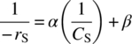
From compilation of these observations, the rate law in Eq. (8.21) was proposed to describe the hydrogenation system independent of catalyst degradation:
where
- k and K are constants.
-
 is the concentration of dissolved hydrogen.
 - CCat is the catalyst concentration (constant for a given experiment).
To interpret this empirical rate law in the context of the reaction mechanism (Scheme 8.8), one can examine Eq. (8.21) and identify two limiting cases for the reaction rate. Considering first the case where KCS ≫ 1, the reaction rate simplifies to a first‐order rate dependence upon the hydrogen concentration, implying that the insertion of hydrogen determines the rate for the catalytic cycle under these conditions. As the alkene concentration is reduced (KCS ≪ 1), the rate law effectively becomes first order in both CS and ![]() . This would be indicative of a limiting dependence of the rate upon the alkene coordination, with a relatively fast equilibrium established for the molecular rearrangement of II and III. The following steps can therefore be written out to support the experimentally observed rate law:
. This would be indicative of a limiting dependence of the rate upon the alkene coordination, with a relatively fast equilibrium established for the molecular rearrangement of II and III. The following steps can therefore be written out to support the experimentally observed rate law:
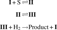
Evaluation of this sequence of elementary steps affords the proposed rate law in Eq. (8.21).
In general, were the reaction mechanism (or mass transfer effects) to be well known at the outset of a study, the need for experimentation would be minimal and would amount only to an exercise of fitting rate coefficients. In practice, the approach of monitoring for rate‐limiting behavior is important in that new mechanistic insights are often gained by observing the chemistry at conditions where apparently “simple” kinetics transition to new regimes. An example of such an occurrence was demonstrated by Blackmond and coworkers for the Heck coupling reaction shown in Scheme 8.9 [74]. The catalytic cycle is nominally consistent with the general catalytic cycle for a cross‐coupling reaction and begins with oxidative addition of p‐bromobenzaldehyde (13) to the dimeric palladacycle catalyst 16, followed by the addition of the olefin butyl acrylate (14) and finally reductive elimination to generate the desired product and regenerate the catalyst. Using reaction calorimetry, Blackmond and coworkers examined this reaction and observed multiple irregularities in the reaction rate in comparison with conventional Heck reaction kinetics. Whereas kinetic analyses of the Heck reaction are usually performed with a large excess of olefin (making the kinetics pseudo‐zero order in olefin), the researchers in this case found that the reaction rate both had a dependence on olefin concentration and was sublinear when the catalyst concentration increased. A profile of the reaction rate with time (shown in Figure 8.10a) revealed the reaction to undergo a transition in rate behavior after about 90% conversion of the aryl bromide.
SCHEME 8.9 Heck coupling reaction of p‐bromobenzaldehyde and n‐butyl acrylate.
FIGURE 8.10 (a) Reaction heat flow as a function of time for Heck reaction in Scheme 8.9 with catalyst 16 and calculated conversion. (b) At 50% conversion, dependence of reaction rate on catalyst 16 and fit to proposed half‐order catalyst dependence (Eq. 8.22).
Source: Reprinted with permission from Rosner et al. [74]. Copyright 2001, American Chemical Society.
Given these observations, the researchers hypothesized the modified catalytic cycle illustrated in Scheme 8.10. The perceived inhibitory effect of operating with increased catalyst was attributed to the equilibrium formation of a [PdLArX]2 dimer after the catalyst had undergone oxidative addition. Equilibrium for this reaction was theorized to significantly favor formation of the dimer. In the limiting case of complete inhibition because of dimer formation, the rate law was proposed to scale with the square root of the total palladium concentration (CPd):
SCHEME 8.10 Modified catalytic cycle for Heck reaction including formation of [PdLArX]2 dimer.
This expression was then incorporated into a comprehensive rate law [74], generating a rate law that would simplify to a first‐order dependence on the kinetics in CPd when KR was small and transition to a half‐order dependence on CPd when KR was large. The model fit is illustrated in Figure 8.10b. The modified rate law suggested that non‐first‐order dependence of the rate on the catalyst would only be observed when oxidative addition of the aryl halide was not limiting. Beyond 90% conversion, the olefin concentration was depleted sufficiently such that the oxidative addition step became rate controlling. Qualitatively similar behavior was observed using the dimeric catalyst 17.
From the discussions in Section 8.2, it should be apparent that in addition to relative reaction rates, other factors such as mass transfer or heat transfer may also contribute to effective rate‐limiting behaviors. An example illustrating the convolution of reaction rate with mass transfer can be found in the case of the Fischer indole reaction shown in Scheme 8.11. The Fischer indole reaction is expected to proceed through a hydrazone intermediate (Scheme 8.12), which exists as a slurry before strong acid drives the cyclization to close the pyrrole ring and form the bicyclic indole [76].
SCHEME 8.11 Fischer indole reaction.

SCHEME 8.12 Proposed pathway for the Fischer indole reaction of Scheme 8.11.
The kinetics of this reaction were studied using reaction calorimetry and off-line HPLC. Multiple small (0.15 equiv.) injections of methane sulfonic acid (MSA) were introduced into a slurry of hydrazone in the calorimeter. Figure 8.11a shows modified calorimetry data indicating the reaction rate data as a function of hydrazone concentration. Each injection of MSA can be thought of and analyzed as an individual batch reaction. Each peak observed in Figure 8.11a is due to an identical spike of MSA, which is nearly depleted after each reaction. Changes in the initial hydrazone concentration allow for calculation of the reaction order in hydrazone during the course of the reaction. Superposition of the reaction profiles from the four MSA injections revealed that the reaction rate was zero order in initial hydrazone concentration and exhibited an overall third‐order behavior when plotted as a function of MSA concentration, as shown in Figure 8.11b (solid line represents the rate profile expected from third‐order kinetics).
FIGURE 8.11 Rate of Fischer indole reaction as a function of (a) overall hydrazone concentration and (b) MSA concentration.
The initial zero‐order kinetics for the Fischer indole reaction with respect to hydrazone were consistent with the rate being solubility limited in hydrazone. To better understand the underlying mechanism impacting the third‐order rate behavior and the effect of dissolution kinetics, the solids in the reaction mixture were removed by filtration, and an identical study was conducted under homogeneous conditions using the dissolved hydrazone in the filtrate. The results of this experiment are shown in Figure 8.12. These results indicated a nearly first‐order dependence of reaction kinetics on hydrazone concentration and second‐order dependence on MSA concentration in the absence of mass transfer limitations. The overall third‐order kinetics observed in Figure 8.11b were in actuality a convolution of second‐order dependence on MSA concentration and first‐order dependence on hydrazone concentration. These results were further validated with IR measurements.
FIGURE 8.12 Plot of Fischer indole reaction rate under homogenous conditions as a function of (a) hydazone and (b) MSA concentration. Dashed lines in (a) and (b) represent first‐ and second‐order curves, respectively.
The methods of reaction profiling need not be reserved to batch kinetic studies only. An example of the analogous approach to model generation in flow was demonstrated by Moore and Jensen [77], who examined the Paal–Knorr reaction summarized in Scheme 8.13 using an automated microreactor system. In the experiment, the two reactants, 2,5‐hexanedione (21) and ethanolamine (22), were delivered independently to a heated microreactor, and the reaction conversion was measured at the exit of the reactor with an in‐line Mettler Toledo ReactIR.

SCHEME 8.13 Scheme for the Paal–Knorr reaction.
Taking advantage of the short mixing and heat transfer times in the microreactor system, the authors allowed the reaction to reach steady state in the flow device and then imposed a gradual reduction in the overall flow rate such that the instantaneous residence time in the reactor increased as the experiment progressed, with the reaction stoichiometry held constant. Reaction kinetics were monitored for 60 minutes using IR spectroscopy, then the reactor temperature set point was increased by 20 °C, and the ramp of flow rate was repeated. This process repeated until all experimental conditions of interest had been evaluated. Temperatures in the range of 50–170 °C and reaction times in the range of 0.5–40 minutes were examined comprehensively and automatically in the span of 8 hours. The resulting product concentration and time profiles are provided in Figure 8.13. These results were transferred to a least squares regression algorithm, which estimated activation energies for the two slow Paal–Knorr reaction steps as EA1 = 12.2 ± 0.4 kJ/mol and EA2 = 20.0 ± 0.9 kJ/mol, respectively.
FIGURE 8.13 Kinetic profiling of the Paal–Knorr reaction in flow with IR spectroscopy.
Source: Reprinted with permission from Moore and Jensen [77]. Copyright 2014, John Wiley and Sons.
This method was later revisited by the same authors in the case of the continuous flow aminocarbonylation of p‐bromobenzonitrile, shown in Scheme 8.14 [78]. With the goal of modeling the factors influencing the formation of either the mono‐amide (26) or the di‐α‐keto amide (27), the authors examined the reaction in the context of both gas pressure and reaction temperature. From preliminary screening results in the microreactor system, the gas–liquid mass transfer rate was found to be non‐limiting in the experimental condition range of interest. Based on this result, the rate‐limiting kinetics were simplified to
where
- k, k1 and kobs are constants
- CPd represented the molar concentration of the active palladium species (relative to initial palladium (CPd)0).
- C24 represented concentration of the aryl halide.
- CCO represented the concentration of carbon monoxide
SCHEME 8.14 Continuous flow aminocarbonylation reaction of p‐bromobenzonitrile.
The reaction was then conducted in a tubular reactor containing stainless steel beads for mixing and was heated in 1 °C increments every 2 minutes from 80 to 160 °C. The reaction effluent was continuously monitored by IR spectroscopy, and principle component analysis (PCA) was used two distinguish the two products from the starting aryl halide. Automated operation resulted in generation of the reaction profile in Figure 8.14, which showed the reaction to afford nearly identical selectivity toward the mono‐ and di‐α‐keto amide products at temperatures less than 120 °C. However, once the temperature climbed to above 120 °C, the selectivity appeared to shift to as much as 2 : 1 in favor of the mono‐amide 26.

FIGURE 8.14 IR‐measured concentration profile for aminocarbonylation products in Scheme 8.14 with increasing tubular reactor temperature (8.3 minutes residence time; 8.3 bar CO).
Source: Reprinted with permission from Moore et al. [78]. Copyright 2016, The Royal Society of Chemistry.
In evaluating the observed results, the researchers first considered the independence of the reaction selectivity at below 120 °C, attributing this observation to the originally proposed limiting oxidative addition kinetics from Eqs. (8.23) to (8.24). For this limiting case, it was found through further experimentation that the rate was linear with the inverse of the CO pressure (due to competition from the reversible reaction of the Pd–ligand catalyst with CO to form [PdLCO]). The observed rate constant from Eq. (8.24) was then simplified to the ratio k1(CPd)0/KCCO (a function of temperature only with CCO in excess), and an effective activation energy for the reaction was estimated deriving from the first‐order dependence of the rate upon C24. Based upon the results at higher temperature conditions, the researchers proposed an alternative mechanistic route that drew upon literature precedent [79], suggesting two competing routes to the formation of the mono‐amide (Scheme 8.15). The “inner” cycle via k2 and k4, by virtue of forming a more entropically favorable intermediate, was hypothesized to become more favorable with increasing temperature. Such a mechanism was shown numerically to support both the enhanced selectivity toward the mono‐amidation product at high temperatures and the pseudo‐first‐order dependence upon the aryl halide concentration at low temperatures upon regression to experimental data. This example cited a two to three times speed improvement compared with conventional flow experimentation and highlights the impact that automation and PAT are having upon kinetic modeling in next‐generation development.
SCHEME 8.15 Catalytic cycle for aminocarbonylation reaction in Scheme 8.14.
8.4.2 Design of Experiments
For cases where a well‐characterized kinetic model may simply be too complex to compile or large volumes of data are too expensive to generate, response surface models constructed from design of experiments (DoE) principles can be invaluable in providing the researcher with basic guidance on the interactions of multiple process inputs and for providing preliminary insight into process optimization. Countless literature examples are available to demonstrate the application of DoE in pharmaceutical process development [80], with emphases placed on initial screening [81], process optimization, and model development. The application of DoE has also become increasingly synonymous in the pharmaceutical industry with the definition of the design space [82]. Though it is to the practitioner's discretion as to how to define a design space, the general approach requires both process knowledge and statistical experimental design tools to identify and confirm an acceptable region of process operation [83]. Many software tools have been introduced to assist in this experimental design process; prominent examples include Design Expert (Stat‐Ease, Inc.), Minitab (Minitab, Inc.), and JMP (SAS).
The goal herein is to show how DoE methods can be selectively applied to model development in the spirit of other case studies already highlighted in this chapter. If the DoE methodology has a fault, it is that those who leverage it can get lost in overestimating the value of statistical models generated from a small sample of experiments. To avoid this trap (particularly for reaction kinetics, which could be otherwise deduced through first principles mechanistic understanding), it is essential that empirical results be examined critically in the context of any simplifications made in generating the original experimental design. An effective use of DoE may be to review the initial experimental data generated and apply the knowledge gained either to a new experimental design or to construction of a model that derives from mechanistic principles.
The DoE process generally begins with the identification of one or more responses (e.g. yields, quality attributes, material properties) to control and the identification of factors/variables (e.g. temperature, time, amount) believed to have the most significant influence upon those responses. Depending upon the number of variables under consideration, it may be prudent to conduct an initial set of screening experiments to prioritize factors and eliminate those with little or no impact upon the targeted outcome. Such a screen could be a full factorial design, where all factors k are considered in combination at high and low levels to afford a total of 2k experimental conditions. Alternatively one could use a fractional factorial design, where the number of high‐ and low‐level experiments is divided by 2n to save experimental time, at the expense of losing some information as to the higher‐order interactions among variables. After refining the list of candidate variables, a more comprehensive set of experiments is then prescribed. Examples could include, but are not limited to, full factorial or higher‐order fractional factorial designs, central composite designs, or Box–Behnken designs. These latter two designs include experiments not situated at the vertices of the experimental design region, which are necessary to detect nonlinearity in individual factors. The prescribed experiments are then executed, and the results are compiled to afford a response surface model that relates the response(s) to the variables in combination. Various statistical tools can be used to quantify the accuracy of the empirical model.
A general example showing the merits of the DoE procedure can be found in Stazi et al. [84], who examined the Koenigs–Knorr glucuronidation of the nitrophenol 28 as shown in Scheme 8.16. Initial efforts to react 28 in the presence of the sugar 29, Ag2O, and 4 Å molecular sieves resulted in very low yields on account of the chelation of the product 30 to the silver ions. It was learned that the yield of 30 could be substantially increased with the use of a chelating amine such as the tetradentate 1,1,4,7,10,10‐hexamethyltriethylenetetramine (HMTTA), but one‐variable‐at‐a‐time optimization and a screen of candidate Ag sources and amines failed to deliver the product 30 in better than 40% yield.
SCHEME 8.16 Koenigs–Knorr glucuronidation reaction.
In light of these results, the researchers decided to apply DoE to identify and optimize the key mechanistic factors in the HMTTA chemistry. Seven factors – precomplexation time for HMTTA and Ag2CO3, reaction time, Ag2CO3 equivalents, HMTTA equivalents, sugar equivalents, amount of molecular sieves, and solvent volume – were proposed to contribute in the reaction to the yield of 30. Whereas a full factorial DoE would have required a minimum 128 experiments, the authors instead proposed a fractional factorial design in which individual variable contributions and pairwise interactions between variables could be assessed with only 11 experiments at the extremes and center of the experimental design space. These initial experiments indicated that the yield depended most significantly upon the precomplexation time and upon the amounts of Ag2CO3, HMTTA, and sugar 29 used in the experiment. A consequence of using such a reduced fractional factorial design, the interaction of Ag2CO3, and the amount of 29 was strongly correlated to the precomplexation time in the preliminary experiments. Because of this and in order to limit the overall number of experiments, the authors elected in subsequent response surface modeling to only consider the three reagents, Ag2CO3, HMTTA, and sugar 29, and to maintain a constant precomplexation time of 60 minutes. A 20‐experiment central composite design was conducted, which sampled from points on both the edges and interior of the experimental space.
Following response surface generation from the results of the three‐factor central composite design, Stazi et al. noted the abnormality of the bimodal dependence of the product 30 upon the additive HMTTA, shown in Figure 8.15a. Such an effect was captured empirically with a cubic polynomial model and was postulated to arise from any of several factors, including the involvement of HMTTA in competing as a ligand for silver ions, in activating the silver source, in deprotonating the phenol 28, and in contributing to the dehydrohalogenation of sugar 29 when used at high concentration. To discern and quantify each of these effects, the researchers conducted additional experiments comparing the complexation of reactant 28 with silver from either Ag2O or Ag2CO3 in the presence or absence of HMTTA. From these studies, the researchers found that the complexation kinetics of 28 with Ag2O are slowed in the presence of HMTTA as the HMTTA competes as a ligand for the silver ions. Instead, however, with Ag2CO3 the rate of complexation increases significantly in the presence of HMTTA, likely because of the increased dissolution of silver salt in the HMTTA system. Finally, the complexation of 28 and with the source Ag2CO3 was assessed as a function of HMTTA equivalents and found to exhibit a maximum as shown in Figure 8.15b. At low loadings of HMTTA, the complexation rate increased with increasing HMTTA charge on account of increased solubility of Ag+ in solution. However, an increase of HMTTA to above approximately 0.7 equiv. led to a decrease in the complexation of 28 as the increased amine competed for the binding to the silver ions. With this added knowledge, the chemistry was optimized to produce 30 on a 3.5 g scale in greater than 85% yield (compared with not more than 40% using traditional one‐variable‐at‐a‐time optimization).

FIGURE 8.15 (a) Influence of stoichiometry of Ag2CO3 and HMTTA on the in situ yield of 30 for 2.42 equiv. sugar 29. (b) Effect of different amounts of HMTTA on complexation equilibria between 28 and Ag2CO3 at reaction times of 2, 4, and 6 hours.
Source: Reprinted with permission from Stazi et al. [84]. Copyright 2004, American Chemical Society.
The use of DoE tools and concepts does not preclude more detailed mechanistic investigation. By nature, mechanistic insights require a greater understanding of underlying science and physics – an understanding that may be accessible for primary reaction pathways but may be difficult to discern for low‐level impurities. In this case, it would seem reasonable that a control strategy could be based on both mechanistic considerations (to account for all that is well‐understood in the reaction system) and empirical considerations (to capture the impact of other, less‐readily characterized factors upon a proposed design space). In utilizing this approach, the question becomes how to define, and then verify, these empirical relationships while accounting for the framework provided by the established mechanistic knowledge. Researchers at Bristol‐Myers Squibb (BMS) have produced several papers [85–87] illustrating an approach to these problems that is consistent with the FDA's guidelines for quality by design [83]. Given that the problem involves determining design space robustness, it should not be a surprise that the methodology relies heavily upon the application of DoE.
An example of this approach was provided by Burt et al. in a case study involving the base‐mediated conversion of an ester to a primary amide [86, 88]. The postulated network is shown in Scheme 8.17. Formation of the drug substance 34 occurs in a multistep sequence: deprotonation of the amidation reagent 31, followed by reaction of the active amide species 32 and amine 31 with the input ester 33 to afford the drug substance 34 and an imide by‐product 35. Both reactions are equilibrium reactions. As hydrolysis with water can cause degradation of the input ester 33 in the presence of base, an orthoester 37 is used to promote chemical removal of water prior to initiation of the amidation reaction, yielding formate 38. However, 38 can react with the amide 32 to produce the imide 35, shifting the equilibrium of the desired pathway away from the formation of the drug substance. The imide 35 can also form via side reactions originating with either the drug substance or a diester impurity 39 introduced in the feed. These last two side reactions also afford bis‐amide species 40 that was the key impurity in the drug substance manufacturing process.

SCHEME 8.17 Network of reactions for base‐mediated conversion of an ester to a primary amide and competing by‐product formation.
Implementation of a multistaged DoE began with the identification of factors most likely to impact product purity; those factors were identified through a process risk assessment as reaction temperature, equivalents of base, initial water content of the feed solution (i.e. prior to chemical water removal), and the amount of diester impurity 39 in the feed. For the initial stage DoE, three of these factors – reaction temperature, base amount, and water amount – were screened in a 23 factorial design. The results of these experiments were applied to estimate temperature‐dependent rate coefficients for the formation of drug substance 34, and its degradation to bis‐amide impurity 40. For this initial stage DoE, input‐related diester impurity 39 was maintained at a uniformly low level to allow for clean regression of kinetic parameters for drug substance degradation to the bis‐amide impurity.
With a preliminary mechanistic model in place, a second stage DoE was undertaken to delineate the limits of the multivariate parameter space (encompassing both process parameter ranges and input quality attributes), affording in‐specification drug substance. A 24−1 fractional factorial design was considered (including the amount of orthoester 37 as a fourth factor), and the diester impurity 39 was included in the reaction at its specification limit in the input ester 33. In a third stage DoE, axial points were assessed for the initial three factors (DoE stage 2 had confirmed that variation of orthoester amount across its univariate PAR was not quality impacting). For DoE stages 2 and 3, key responses included levels of residual input ester 33 and bis‐amide impurity 40, both in process and in the isolated product, and the isolated drug substance yield. The combined results of DoE stages 2 and 3 gave indication of the curvature of the system and delineated two regions of the multivariate parameter space corresponding to process failure modes: a combination of high reaction temperature and high base for formation of bis‐amide impurity 40 and a combination of high reaction temperature and low base for unreacted ester 33.
In addition to identifying a subset of the multivariate parameter space that afforded in‐specification drug substance, the BMS team recognized that the compilation of results from their multistaged DoE could support the development of a hybrid mechanistic and empirical process chemistry model. Elementary rate expressions were assumed for the formation of drug substance 34, the imide 35, and the degradation of drug substance to bis‐amide 40. The rate of bis‐amide impurity generation from input‐related diester 39 was quite fast, and the level of the diester itself was small; hence the model parameters for the elementary rate expressions were first regressed, and then an empirical component was applied to the mechanistic modeling results to account for the varying magnitude of bis‐amide impurity resulting from the initial presence of the diester in the feed. Once a hybrid model was compiled, the BMS team was able to verify the parameter estimates with additional experimentation. The resultant hybrid process chemistry model was leveraged to guide the selection and verification of a design space for the drug substance manufacturing process.
8.4.3 Parameter Estimation and Model Discrimination
The preceding examples illustrate both the advantages and disadvantages of leveraging DoE in process development. DoE is an efficient tool for surveying the impact of several (perhaps interacting) factors upon specified responses. As exemplified, the DoE process can often reveal new regions of the experimental space that are overlooked when changing only a single variable at a time, making it more likely that a better process optimum is found and that the empirical kinetics more comprehensively represent system behavior across a robust design space. A negative of the approach is that without proper vetting of candidate variables, the number of experiments needed to complete the DoE can quickly become unmanageable. Choosing all or the majority of these experiments at the outset can be costly as well, as experiments will inevitably be chosen that either (i) are non‐informative in that they do not generate knowledge beyond what has already been learned from previous experiments or (ii) are nonoptimal and hence unlikely to be relevant for process optimization or design space considerations. To address scalability concerns, there is no substitute for having access to a kinetic model describing the process in detail.
The question may be asked then as to how to bridge the more general knowledge gained through the DoE approach with established methods for kinetic model development, enabling greater process understanding to be gained in less experimental time. One route to achieving this is through the use of feedback optimization, wherein one or a handful of selected experiments are executed, then the data are analyzed, and a new experiment is proposed, which should – given the prior data collected – produce the most information to support or refute the proposed model. The selected experiment is then conducted and the procedure repeats. Though exceptions exist [89–91], such a sequential improvement methodology is usually too tedious to implement when developing processes in batch when factoring time for sample preparation/analysis and off-line process modeling. With continuous flow, however, the integration of equipment control, analytical instrumentation, and computational tools can greatly facilitate the process of iterative optimization or model construction, shortening process development lead times from weeks to a few hours or days [92, 93].
Justification of the feedback optimization approach requires a more generalizable understanding of the method for model regression. Such a method to nonlinear model parameter estimation is documented, for instance, in Ref. [5] and involves minimization of the sum of squared residuals between observed (measured) responses, yi, and predicted responses, ![]() , for a set of conducted experiments, indexed here by u:
, for a set of conducted experiments, indexed here by u:

Here, θ is a group of parameters (e.g. activation energies and pre‐exponential factors) relating the adjustable variables in the reaction to the predicted responses. The term Vεu is a weighting matrix that approximates the relative uncertainty in each measured response for the experimental conditions u. Estimation of the elements of Vεu comes from taking the variance or covariance expected for each pair of responses upon repeated experimentation at the set of experimental conditions. For cases where it is impractical to conduct many replicate experiments, an estimate for Vεu can sometimes be employed by calculating a general covariance matrix Vε with elements (Vε)ij as follows:

Because this calculation assumes the best‐fit parameters in the models describing ![]() and
and ![]() , Eq. (8.26) must be evaluated iteratively with the optimization in Eq. (8.25).
, Eq. (8.26) must be evaluated iteratively with the optimization in Eq. (8.25).
Independent of the variance from experiment to experiment, precise estimation of kinetic parameters is also contingent upon selection of the correct experiments to distinguish different elements of the model from one another. This should be intuitive given the many examples in this chapter of changes in an apparent reaction model that are only observable at particular processing conditions. The sensitivity of a model (Xu) is a quantitative measurement of how much each model prediction changes as its defining parameters are varied:
The sensitivity matrix is not a constant but instead changes as the experimental conditions u change. A larger magnitude value of (Xu)ip (either positive or negative) implies that a small change in the parameter value will be reflected in a greater change in the observed response ![]() . Such a condition makes it favorable to estimate model parameters or distinguish between models, as subtle differences in the model will translate to appreciable differences in the experimental outcomes.
. Such a condition makes it favorable to estimate model parameters or distinguish between models, as subtle differences in the model will translate to appreciable differences in the experimental outcomes.
Accounting for both the sensitivity of the experimental outcome to the model and the variability of the experiment itself, the total amount of information that can be collected during the model development process is given by the Fisher information matrix in Eq. (8.28):

Among the important properties of this matrix is that its inverse Z−1 corresponds to the covariance matrix of the estimated parameter values, meaning that the elements of Z give a quantifiable measure as to with how much certainty the proposed model and kinetic coefficients describe the experimental data. In sequential experimental design, the goal then becomes selection of new experiments that can lead to the smallest uncertainty in the model, i.e. by selecting experiments that minimize the size of elements in Z−1. A widely used metric is D‐optimality, which aims to shrink total volume of the region of uncertainty for all model parameters as shown in Eq. (8.29):
The addition of experimental data to the optimization in Eq. (8.29) serves to (hopefully) lessen |Z−1|. By lessening |Z−1|, the variance and covariance estimates for the model parameters are reduced, and hence the model is supported to greater precision. With further refinement of the model parameters, the ability of the model to predict sensitivity coefficients in future experiments should improve, meaning that the quality of experimental conditions chosen to inform model development should improve as well.
An example employing the D‐optimal design method for kinetic model development was demonstrated by Reizman and Jensen in consideration of the series–parallel nucleophilic aromatic substitution reaction pathway shown in Scheme 8.18 [94]. Reagents 2,4‐dichloropyrimidine (41) and morpholine (25) were reacted in an automated flow system. At the outlet of the flow reactor, the concentrations of pyrimidine derivatives 41, 42, 43, and 44 were measured by online HPLC. Results of this analysis were supplied to a computer algorithm, which estimated kinetic parameters assuming elementary second‐order reaction kinetics of the reactions of morpholine with 41, 42, and 43. After an initial set of factorial experiments, the computer algorithm selected a new set of experimental conditions (flow rates and temperature) that would most greatly reduce the uncertainty in the kinetic model parameters. These experimental conditions were automatically provided to the continuous flow system, which executed the new experiment to allow the feedback loop to repeat.
SCHEME 8.18 Nucleophilic aromatic substitution reaction pathway for 2,4‐dichloropyrimidine and morpholine.
The initial factorial design afforded reasonable estimates for the pre‐exponential and activation energy parameters associated with k1 and k2, with reported uncertainties in parameter values not exceeding ±12%. This same factorial design, however, proved to be unacceptable for resolving the rate of formation of the disubstituted product 44 and in the estimation of parameters associated with k3 and k4. Not surprisingly, the majority of ensuing feedback experiments were selected at higher temperatures and longer reaction times, where a greater yield of the product 44 was expected. After an additional 12 optimal experiments, the relative uncertainty on the activation energies for k1 and k2 had been reduced to at most ±6% and for k3 and k4 to at most ±14%, and qualitatively reasonable model predictions were obtained. For further resolution of the kinetic parameters, Reizman and Jensen reverted to the more “traditional” method of kinetic estimation by isolating each of the intermediate monosubstituted products and then using the automated flow system to estimate the rate constant parameters associated with the one‐step conversion of these intermediates to the disubstituted product 44. The rate parameters for k3 and k4 and their uncertainties were then supplied to a final all‐at‐once automated parameter fitting exercise that afforded rate coefficients with no more than ±4% error. In total, 78 automated experiments were needed to fit the 8‐parameter model.
The parameter estimation approach can be expanded to model discrimination using the goodness‐of‐fit metric χ2. To compare two or more candidate models, a reduced χ2 value is calculated for each model using sum‐of‐squares residuals as follows:

The reduced χ2 is scaled by the available degrees of freedom and therefore is reduced both for a better model fit and the use of fewer model parameters. In this regard it is unfavorable to add more parameters to a model without improving upon the goodness of fit.
The use of the goodness‐of‐fit approach was demonstrated by Greiner and Ternbach for the hydrogenation chemistry in Scheme 8.19 [95]. The homogeneous rhodium catalyst complex {[Rh(PyrPhos)‐(COD)]BF4;45‐COD} was used in the study. The catalyst 45 is liberated from the precatalyst complex before entering into the catalytic cycle and facilitating the reduction of N‐acetylaminocinnamic acid (46) to 47. The authors proposed inclusion of first‐order kinetics describing both the activation and deactivation of 45 in the model:

SCHEME 8.19 Rhodium‐catalyzed hydrogenation of N‐acetylaminocinnamic acid.

SCHEME 8.20 Diels–Alder reaction of isoprene and maleic anhydride.
Likewise the consumption of 46 was hypothesized to be dependent on the equilibria of intermediates of the catalytic cycle. A general form of the rate expression was assumed to be:
Six candidate expressions for R were proposed, as summarized in Table 8.4. All expressions included an equilibrium binding constant for 46 to the catalyst, K, and a few included additional inhibitive equilibrium constants for binding to the reactant 46 (Ki,46) or the product 47 (Ki,47). Best‐fit parameters and reduced χ2 values were then calculated for each proposed model (also Table 8.4). Overall minimal χ2 values were found in cases where catalyst deactivation was included in the model, namely, in models 5 and 6. Model 6, which included the maximum six parameters, gave a slightly improved model fit in comparison with model 5, but the authors questioned the legitimacy of the predicted inhibition kinetics for the more advanced model. Based on simulations of the optimized models, the authors suggested that increasing the concentration of the substrate 46 would be necessary in order to better discriminate between models 5 and 6. Such experiments would be limited by the solubility of 46 in the solvent methanol.
TABLE 8.4 Best‐Fit Parameters for Candidate Rate Models Describing Hydrogenation of N‐Acetylaminocinnamic Acid
Source: Reprinted with permission from Greiner and Ternbach [95]. Copyright 2004, John Wiley and Sons.
| Model | 1 | 2 | 3 | 4 | 5 | 6 |
| Description | Michaelis–Menten | Substrate Surplus Inhibition | Competitive Product Inhibition | Both Inhibition Types | Model 1 with Deactivation | Model 4 with Deactivation |
| R in Eq. (8.32) | K + C46 |  |
K + C46 |  |
||
| kact (h−1) | 1.541 ± 0.012 | 1.566 ± 0.012 | 1.403 ± 0.010 | 1.404 ± 0.010 | 1.045 ± 0.007 | 1.103 ± 0.008 |
| kdeact (h−1) | — | — | — | — | 0.012 ± 9E‐5 | 0.012 ± 13E‐5 |
| K (mM) | 25.3 ± 0.11 | 27.4 ± 0.18 | 5.96 ± 0.17 | 7.61 ± 0.21 | 17.6 ± 0.09 | 20.5 ± 0.23 |
| νmax (min−1) | 10.8 ± 0.006 | 11.0 ± 0.013 | 10.7 ± 0.005 | 10.9 ± 0.012 | 11.6 ± 0.009 | 12.0 ± 0.019 |
| Ki,46 (M) | — | 40a | — | 40a | — | 14.8 ± 0.45 |
| Ki,47 (M) | — | — | 0.177 ± 0.007 | 0.221 ± 0.008 | — | 11.8 ± 2.6 |
| χ2 | 7.0 | 6.8 | 4.3 | 4.2 | 3.4 | 3.0 |
95% accuracy bounds are provided for parameters and χ2 values are provided for models.
aValues are at upper boundary.
The observation that additional experiments are needed in untested regions of the experimental space is almost ubiquitous to kinetic model discrimination and is reflective of the challenges of scale‐up. Statistical tools for model discrimination can help in this regard, provided that the candidate models incorporate the relevant information needed for scale‐up. Consider as an example the simplified case of the Diels–Alder reaction of isoprene (48) and maleic anhydride (49) studied by McMullen and Jensen [96]. The researchers were interested in using an automated flow system to discriminate among four candidate reaction rate laws:
The reactants and the solvent DMF were automatically delivered to a microreactor and analyzed online by HPLC. The result of the analysis was returned to a computer algorithm that determined best‐fit parameters for the four candidate models and then selected new experimental conditions that would most greatly accentuate the differences between the models. These new reaction conditions were transferred to the automated system, and the process repeated.
To compare candidate models, McMullen and Jensen chose to use a Bayesian approach first introduced by Box and Hill [97]. A half‐factorial, four‐experiment DoE was prescribed to calculate these variances and generate initial model predictions; after this design, only two optimized experiments were needed to confirm with greater than 99% certainty that the second‐order model given by Eq. (8.33) was the most representative of the four candidate models. (Note that even though Eq. (8.36) is the reversible form of Eq. (8.33), the Bayesian approach was able to discriminate this model by demonstrating kIV, r to be effectively zero.) Figure 8.16 shows how, entering the fifth experiment (i.e. the first optimized experiment), the probability distributions for the isoprene concentration at the reactor outlet for the first three models under consideration were nearly overlapped, indicating that any of these models could reasonably describe the data. However, given the result observed in the fifth experiment, a much greater discrepancy in the probability distributions among models was observed in the ensuing experiment. The result of this experiment was consistent only with the second‐order overall model, Eq. (8.33). Once this model was selected, the activation energy and pre‐exponential parameters for kI were further refined by conducting iterative experiments with feedback.

FIGURE 8.16 Probability distribution maps showing likelihood of output isoprene concentration for a given kinetic model after (a) fifth and (b) sixth automated model reduction experiments for the Diels–Alder reaction. Fifth experiment selected conditions: τ = 1 minutes, C48 = C49 = 0.5 M. Sixth experiment selected conditions: τ = 1 minutes, C48 = 2.0 M, C49 = 1.5 M.
Source: Reprinted with permission from McMullen and Jensen [96]. Copyright 2011, American Chemical Society.
Following the kinetic study, the researchers engaged in a 500‐fold scale‐up of the Diels–Alder reaction to the 60 ml Corning Advanced Flow Reactor (AFR) system. To accurately scale to the larger continuous reactor, both the dispersion in the reactor and the heat transfer rate for the AFR needed to be estimated. The dispersion coefficient, D, was measured by measuring the tracer signal following a pulse injection in the AFR. This value was then used as an input into the dispersion model for a laminar flow reactor. To account for the rate of heat transfer, the heat of reaction for the Diels–Alder chemistry and the heat transfer coefficient for the AFR were both estimated from literature values. Using these approximations, the product concentrations at four different experimental conditions were evaluated numerically and found to be in good agreement (within 3%) with the experimental results found in the AFR. Overall, this example demonstrates the efficiency of scale‐up that can be achieved with limited experimental effort and through the applications of automation, optimal experimental design, and continuous flow technology.
8.5 EMERGING AREAS FOR INNOVATION AND IMPLEMENTATION
Notwithstanding the innovative approaches to reaction kinetic characterization already discussed in this chapter, it is recognized that best‐practice approaches will continue to evolve as new technologies enter into the process development space. This section considers a few of the emerging challenges impacting the pharmaceutical industry and a select group of the disruptive technologies expected to grow in utilization in response to these challenges.
8.5.1 Computational and Statistical Tools for Model Development
As chemical systems increase in complexity – both in terms of molecular structures and in the modes of implementation – the roles of computational modeling and data mining will become more prominent in the description of kinetic phenomena. As of 2018, complete in silico modeling of a chemical reaction system relevant to the pharmaceutical industry has yet to be realized [98]; however progress by way of computational chemistry and in particular with the use of density functional theory (DFT) [99] has led to breakthroughs in optimizing reaction selectivity and substrate selection, predicting impurity formation, and deciphering mechanisms in both organocatalysis and organometallic catalysis [100]. Among the more notable DFT tools for predicting reaction mechanisms are the artificial force‐induced reaction method [101] and the ab initio nanoreactor [102]. For faster elucidation of reaction mechanisms and/or evaluation of larger molecular systems, more heuristic graph‐based methods [103] and machine learning‐based methods [104] have been introduced. Regarding solvent selection for chemical reactions, Adjiman and colleagues presented a quantum mechanical computer‐aided molecular design (QM‐CAMD) methodology for identification of rate‐accelerating solvents in application to a Menschutkin reaction [105]. A virtual screen of over 1300 candidate solvents and afforded a 40% improvement in reaction rate compared with an initial six‐solvent screen. Despite these advancements, uptake of quantum mechanical simulation technologies into industrial process development remains slow on account of lack of speed of the simulation in comparison with lab experimentation, restrictions on maximum molecule size and computing power, and simply a lack of accessibility to the non‐computational specialist. As the accessibility and accuracy of molecular‐scale simulation improve, the field of process development should experience an increased impact of these tools in areas such as reaction optimization, solubility prediction, and prediction of mass transfer effects.
Apart from more sophisticated first principles and computation‐rich models, research in high‐throughput reaction development is progressing in the use of statistical tools to augment the information extracted from DoE methodologies. In the optimization of new chemical reactions, the use of PCA has already been demonstrated as an efficient tool for quantifying shared properties of discrete factors, such as solvent attributes or ligand properties [106–108]. The PCA technique reduces a range of physical properties for these discrete variables to a few (perhaps 1–3) nonphysical descriptors that can be treated continuously like the factors normally incorporated into DoE optimization. Carlson was the first to propose the combination of PCA with DoE for the purpose of optimizing solvent selection for chemical reactions [107, 109]. This approach enables a discrete parameter, namely, solvent identity, to be treated as a continuous parameter on the basis of principal component scores that are derived from loading vectors encompassing a multivariate range of physicochemical solvent properties. Exploration of a solvent system described by two or three principal components can be achieved by investigating five or nine solvents, respectively (with solvents selected based on their PCA scores to best approximate a 22 or 23 factorial design, respectively, plus the inclusion of a center point).
A publication from AstraZeneca describes an updated corporate solvent selection guide consisting of a PCA‐based interactive tool [110]. In contrast to previously published pharmaceutical solvent selection guides that focused predominantly upon occupational health, safety, and environmental considerations [111], this interactive solvent selection tool allows for consideration of a broader range of selection criteria. The PCA solvent map was constructed on the basis of 272 solvents and 30 solvent properties. Three principal components captured 70% of the variation in the solvent property data. Literature‐derived examples of reactions exhibiting significant variation in rate or selectivity as a function of solvent were retrospectively applied to the PCA solvent map. In one example, the rate of the SNAr reaction of 4‐fluoronitrobenzene with azide anion was increased by six orders of magnitude upon moving from methanol to hexamethylphosphoramide (HMPA) as solvent [112]. Figure 8.17a shows how the principal component score plots reflect the observed trend in relative reaction rate as the PCA solvent space is traversed. A second example assessed the selectivity of O‐ versus C‐alkylation of 2‐naphtholate by benzyl bromide in a range of solvents (Figure 8.17b) [113]. In this case the O‐alkylation selectivity was adjusted from 7 to 97% upon moving from 2,2,2‐trifluoroethanol to N,N‐dimethylformamide (DMF).
FIGURE 8.17 (a) Reaction rate of 4‐fluoronitrobenzene with azide anion. (b) O‐Alkylation selectivity.
Source: Reprinted with permission from Diorazio et al. [110]. Copyright 2016, American Chemical Society.
In addition to solvent selection, the coupling of PCA with DoE has accelerated the understanding of how solvent and ligand properties contribute to optimal performance in industrially relevant examples such as Suzuki–Miyaura, Heck, Buchwald–Hartwig, Ullman, SNAr, and borrowing hydrogen reactions [109, 114, 115]. Researchers at GSK have also demonstrated how PCA and projection to latent structure (PLS) models can used to diagnose regions of the experimental design space where impurity formation is most prevalent, through the augmentation of response surface models with selected spiking studies [116].
The merger of discrete and continuous factors into automated kinetic modeling is an intuitive next step for reaction optimization platforms. Though a one‐stop machine for chemical optimization and scale‐up is still far from reach, automated on‐demand synthesis [117, 118] and automated reaction optimization for both continuous and discrete factors [119, 120] are emerging technologies. In the latter, even black box optimal experimental design approaches to reaction optimization have shown a propensity to identify shared response surface model attributes among solvents and catalysts with known physical property similarities. With further development, this technology could be interfaced with PCA tools or even more advanced first principles or machine learning [121] tools in the development of more physically meaningful kinetic models. For this technology to be successful, collaborative efforts between engineers and chemists will be needed in order to build optimization programs that mirror the wealth of knowledge available to the scientist when proposing new mechanisms and candidate reaction pathways.
8.5.2 Integrated Process Control in Pharmaceutical Manufacturing
Increased emphasis on real‐time process control in pharmaceutical manufacturing has stimulated the development of more expansive and robust process models. Guidance [122, 123] introduced in the early 2000s by the Food and Drug Administration (FDA) has led pharmaceutical manufacturers to examine production more holistically in terms of how the variability of process inputs and controls affects end quality. Among the important metrics used by the industry to propose and verify design spaces and demonstrate process robustness are the statistics‐based DoE and mechanistic process modeling [124]. Recent studies have shown an influx of mechanistic modeling approaches to understand important process variables and define the feasible region by constructing probability maps (see, for example, Garcia et al. [84] and Changi et al. [46]). Factors supporting the use of mechanistic models in these exercises include the ability to quantify the risk associated with different process variations (using sensitivity analyses as presented in Section 8.4) and the ability to guide decision making during processing with the use of higher‐level control architectures incorporating data derived from real‐time (or near real‐time) PAT.
The FDA has recognized the importance of models as a tool to assist regulatory submission. The implementation of integrated process diagnostic and control systems in manufacturing will be among the most important drivers for mechanistic modeling in the pharmaceutical industry. Applicable for all manufacturing – but particularly in the case of continuous manufacturing – the coupling of multiple reaction, separation, and/or crystallization steps in a synthetic route dictates the need for predictive understanding of the effects that changes in materials and upstream processing can have on downstream processes and the final product. These changes, when diagnosed through PAT, can be fed to the process model to induce automated process manipulations utilizing feedforward control (changing a downstream operation on account of a change in an upstream material property), feedback control (a corrective change made to the upstream process), or combinations thereof. Examples of how modeling can be used to steer the process toward optimality can be found prominently in crystallization [125, 126] and tablet manufacturing [127–129] literature, but these techniques apply to all areas of pharmaceutical product manufacturing and are becoming key factors in the development of a fully integrated pharmaceutical control strategy [130].
A few plant‐wide feedback and feedforward control strategies utilizing PAT, automation, and process modeling have been presented and have mainly been driven by advances in continuous processing. Lakerveld et al. [131] provided insight into how both local and supervisory controls were used in an end‐to‐end continuous pilot plant. The controller design ensured fast control of critical process parameters, while slower and more overarching process adjustments ensured continuous satisfaction of the product's critical quality attributes. Tools for comprehensive process modeling were developed by Rolandi and Romagnoli [132, 133], but overall the literature to date has been scarce on examples of real‐time process modeling and control applied to chemical synthesis processes. There is an expectation that this will change as integrated pharmaceutical processing grows into a mature technology in the coming years and the importance of process modeling continues to be emphasized by regulatory agencies, as has been the case in previous FDA guidance [134].
8.6 CONCLUSIONS
In summary, the preceding examples highlight the importance of understanding the interplay of chemical transformations with physical rate processes in the context of successful process development, commercial scale‐up, and manufacturing. Although every chemical system introduces new challenges, continued use of the characterization and numerical tools presented herein should enable a more systematic approach to the diagnosis of competing rate effects. Teamwork between chemists and engineers is invaluable in these efforts.
8.7 QUESTIONS
- Derive the expression for kLa (gas–liquid).
The mass transfer from the gas phase to the liquid phase can be described as shown:

where
- Ct is the solution‐phase concentration of the gas at a given time.
- Csat is the equilibrium concentration of the gas in solution.
Integrating the above expression yields the following expression:

where
- Co is the concentration of the gas in solution at t = 0.
- no is the moles of gas initially in solution.
- nt is the moles of gas in solution at a given time t.
- nsat is the moles of gas in solution at the saturation point.
Mass balance for the gas yields the following:
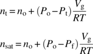
Substitution of the mass balance equation above yields the following expression for kLa:
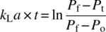
- For a reaction with a first‐order rate law, develop a rate expression that integrates the mass transfer constant for transport across the solid–liquid interface and the intrinsic reaction kinetics.
The rate of diffusion across the boundary layer is defined as follows:

where C∞and CI are the bulk and interface concentrations, respectively. The reaction rate for a power law rate model can be described as follows:

Equating the above two expressions and solving for CI yields the following expression:
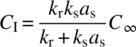
Substitution of this expression into the equation for Rrxn yields the following:
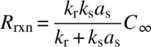
- Show that for the elementary reaction steps below, the overall reaction rate law can be simplified to Eq. (8.21):
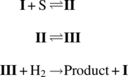
(Hint: The total amount of catalytic species I, II, and III is conserved.)
For the catalytic cycle above, all intermediate species must be generated and consumed at the same rate in order to afford the overall reaction:

The reactions to produce II and III are both in equilibrium; hence we know that


For convenience, we will use the final elementary step to define the overall rate:

Of course CIII is not easily measured before or during the reaction. We do know, however, the total amount of catalyst (Ccat) in the reactor. With some rearranging, an expression for Ccat can be substituted into the rate expression above in place of CIII:

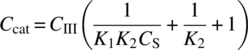
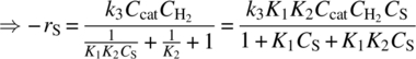
This expression can be simplified further by assuming that the equilibrium between species II and III is shifted toward the intermediate III, such that K2 >> 1 and K1K2CS >> K1CS. For simplicity, define k = k3 and K = K1K2 to afford the rate law:

REFERENCES
- 1. Smith, M.B. (2013). March's Advanced Organic Chemistry: Reactions, Mechanisms, and Structure, 7e. Hoboken, NJ: Wiley.
- 2. Astarita, G. (1967). Mass Transfer with Chemical Reaction. Amsterdam: Elsevier.
- 3. Dankwerts, P.V. (1970). Gas‐Liquid Reactions. New York: McGraw‐Hill.
- 4. Levenspiel, O. (1999). Chemical Reaction Engineering, 3e. Hoboken, NJ: Wiley.
- 5. Froment, G.F. and Bischoff, K.B. (1990). Chemical Reactor Analysis and Design, 2e. New York: Wiley.
- 6. Masel, R.I. (2001). Chemical Kinetics and Catalysis. New York: Wiley.
- 7. Carey, J.S., Laffan, D., Thomson, C., and Williams, M.T. (2006). Org. Biomol. Chem. 4: 2337–2347.
- 8. Roberge, D.M. (2004). Org. Process Res. Dev. 8: 1049–1053.
- 9. Mascia, M., Heider, P.L., Zhang, H. et al. (2013). Angew. Chem. Int. Ed. 52: 12359–12363.
- 10. Cole, K.P., Groh, J.M., Johnson, M.D. et al. (2017). Science 356: 1144–1150.
- 11. Lee, S.L., O'Connor, T.F., Yang, X. et al. (2015). J. Pharm. Innov. 10: 191–199.
- 12. Schaber, S.D., Gerogiorgis, D.I., Ramachandran, R. et al. (2011). Ind. Eng. Chem. Res. 50: 10083–10092.
- 13. Fogler, H.S. (2006). Elements of Chemical Reaction Engineering, 4e. Upper Saddle River, NJ: Pearson Education.
- 14. Steinfeld, J.I., Francisco, J.S., and Hase, W.L. (1999). Chemical Kinetics and Dynamics, 2e. Upper Saddle River, NJ: Pearson Education.
- 15. Reichardt, C. and Welton, T. (2011). Solvents and Solvent Effects in Organic Chemistry, 4e. Weinheim: Wiley‐VCH.
- 16. Niemeier, J.K., Rothhaar, R.R., Vicenzi, J.T., and Werner, J.A. (2014). Org. Process Res. Dev. 18: 410–416.
- 17. Mills, P.L. and Chaudhari, R.V. (1997). Catal. Today 37: 367–404.
- 18. Hartman, R.L., McMullen, J.P., and Jensen, K.F. (2011). Angew. Chem. Int. Ed. 50: 7502–7519.
- 19. Nienow, A.W. (1975). Chem. Eng. J. 9: 153–160.
- 20. Paul, E.L., Atiemo‐Obeng, V.A., and Kresta, S.M. (2004). Handbook of Industrial Mixing: Science and Practice. Hoboken, NJ: Wiley.
- 21. Barker, J.J. and Treybel, R.E. (1960). AIChE J. 6: 289–295.
- 22. Harriott, P. (1962). AIChE J. 8: 93–101.
- 23. Harriott, P. (1962). AIChE J. 8: 101–102.
- 24. Brian, P.L.T., Hales, H.B., and Sherwood, T.K. (1969). AIChE J. 15: 727–733.
- 25. Davies, J.T. (1986). Chem. Eng. Process. 20: 175–181.
- 26. Marrone, G.M. and Kirwan, D.J. (1986). AIChE J. 32: 523–525.
- 27. Armenante, P.M. and Kirwan, D.J. (1989). Chem. Eng. Sci. 44: 2781–2796.
- 28. Tamas, A., Martagiu, R., and Minea, R. (2007). Chem. Bull. “POLITEHNICA” Univ. (Timisoara) 52: 133–138.
- 29. Garside, J., Mersmann, A., and Nyvlt, J. (2002). Measurement of Crystal Growth and Nucleation Rates, 2e. Rugby: Institution of Chemical Engineers.
- 30. Green, D.W. and Perry, R.H. (2008). Perry's Chemical Engineering Handbook, 8e, 7–19. New York: McGraw‐Hill.
- 31. Singh, U.K., Pietz, M.A., and Kopach, M. (2009). Org. Process Res. Dev. 13: 276–279.
- 32. Zwietering, T.N. (1958). Chem. Eng. Sci. 8: 244–253.
- 33. Changi, S. and Wong, S.‐W. (2016). Org. Process Res. Dev. 20: 525–539.
- 34. Bourne, J.R. (2003). Org. Process Res. Dev. 7: 471–508.
- 35. Johnson, B.K. and Prud’homme, R.K. (2003). AIChE J. 49: 2264–2282.
- 36. Mahajan, A.J. and Kirwan, D.J. (1996). AIChE J. 42: 1801–1814.
- 37. Singh, U.K., Spencer, G., Osifchin, R. et al. (2005). Ind. Eng. Chem. Res. 44: 4068–4074.
- 38. Bockhorn, H., Mewes, D., Peukert, W., and Warnecke, H.‐J. (eds.) (2010). Micro and Macro Mixing: Analysis, Simulation and Numerical Calculation. Berlin, Heidelberg: Springer‐Verlag.
- 39. Deimling, A., Karandikar, B.M., Shah, Y.T., and Carr, N.L. (1984). Chem. Eng. J. 29: 127–140.
- 40. Oldshue, J.Y. (1980). Chem. Eng. Prog. 76: 60–64.
- 41. Johnson, M.D., May, S.A., Haeberle, B. et al. (2016). Org. Process Res. Dev. 20: 1305–1320.
- 42. Hickman, D.A., Holbrook, M.T., Mistretta, S., and Rozeveld, S.J. (2013). Ind. Eng. Chem. Res. 52: 15287–15292.
- 43. Rode, C.V., Vaidya, M.J., and Chaudhari, R.V. (1999). Org. Process Res. Dev. 3: 465–470.
- 44. Smith, J.M., Van Ness, H.C., and Abbott, M.M. (2005). Introduction to Chemical Engineering Thermodynamics, 7e. New York: McGraw‐Hill.
- 45. Delgado, J.M.P.Q. (2006). Heat Mass Transfer. 42: 279–310.
- 46. Changi, S.M., Yokozawa, T., Yamamoto, T. et al. (2017). React. Chem. Eng. 2: 720–739.
- 47. Blackmond, D.G. (2005). Angew. Chem. Int. Ed. 44: 4302–4320.
- 48. Mathew, J.S., Klussmann, M., Iwamura, H. et al. (2005). J. Org. Chem. 71: 4711–4722.
- 49. Shekhar, S., Ryberg, P., Hartwig, J.F. et al. (2006). J. Am. Chem. Soc. 128: 3584–3591.
- 50. Singh, U.K., Strieter, E.R., Blackmond, D.G., and Buchwald, S.L. (2002). J. Am. Chem. Soc. 124: 14104–14114.
- 51. Zogg, A., Fischer, U., and Hungerbuhler, K. (2003). Ind. Eng. Chem. Res. 42: 767–776.
- 52. Boddington, T., Chia, H.A., Halford‐Maw, P. et al. (1992). Thermochim. Acta. 195: 365–372.
- 53. LeBlond, C., Wang, J., Larsen, R. et al. (1998). Top. Catal. 5: 149–158.
- 54. Chung, R. and Hein, J.E. (2017). Top. Catal. 60: 594–608.
- 55. Stoessel, F. (2008). Thermal Safety of Chemical Processes: Risk Assessment and Process Design. Weinheim: Wiley‐VCH.
- 56. Simon, L.L., Pataki, H., Marosi, G. et al. (2015). Org. Process Res. Dev. 19: 3–62.
- 57. Chanda, A., Daly, A.M., Foley, D.A. et al. (2015). Org. Process Res. Dev. 19: 63–83.
- 58. Center for Drug Evaluation and Research (U.S.); Center for Veterinary Medicine (U.S.); United States. Food and Drug Administration. Office of Regulatory Affairs (2004). Guidance for Industry: PAT – A Framework for Innovative Pharmaceutical Development, Manufacturing, and Quality Assurance. Rockville, MD: Food and Drug Administration.
- 59. Esmonde‐White, K.A., Cuellar, M., Uerpmann, C. et al. (2017). Anal. Bioanal. Chem. 409: 637–649.
- 60. Singh, K. and Blümich, B. (2016). Trends Anal. Chem. 83: 12–26.
- 61. Gouilleux, B., Charrier, B., Akoka, S. et al. (2016). Trends Anal. Chem. 83: 65–75.
- 62. Foley, D.A. and Dunn, A.L. (2016). Zell MT. Magn. Reson. Chem. 54: 451–456.
- 63. Brum, J. and Dell'Orco, P. (1998). Rapid Commun. Mass Spectrom. 12: 741–745.
- 64. Dell'Orco, P., Brum, J., Matuoka, R. et al. (1999). Anal. Chem. 71: 5165–5170.
- 65. Brum, J., Dell'Orco, P., Lapka, S. et al. (2001). Rapid Commun. Mass Spetrom. 15: 1548–1553.
- 66. Muske, K.R., Badlani, M., Dell'Orco, P.C., and Brum, J. (2004). Chem. Eng. Sci. 59: 1167–1180.
- 67. Snyder, D.T., Pulliam, C.J., Ouyang, Z., and Cooks, R.G. (2016). Anal. Chem. 88: 2–29.
- 68. Ray, A., Bristow, T., Whitmore, C., and Mosely, J. (2018). Mass Spec. Rev. 37: 565–579.
- 69. Theron, R., Wu, Y., Yunker, L.P.E. et al. (2016). ACS Catal. 6: 6911–6917.
- 70. Schafer, W.A., Hobbs, S., Rehm, J. et al. (2007). Org. Process Res. Dev. 11: 870–876.
- 71. Welch, C.J., Gong, X., Schafer, W. et al. (2010). Tetrahedron Asymmetr. 21: 1674–1681.
- 72. Zawatzky, K., Grosser, S., and Welch, C.J. (2017). Tetrahedron 73: 5048–5053.
- 73. Foley, D.A., Wang, J., Maranzano, B. et al. (2013). Anal. Chem. 85: 8928–8932.
- 74. Rosner, T., Le Bars, J., Pfaltz, A., and Blackmond, D.G. (2001). J. Am. Chem. Soc. 123: 1848–1855.
- 75. O'Connor, C. and Wilkinson, G. (1968). J. Chem. Soc. A. 2665–2671.
- 76. Hughes, D. and Zhao, D. (1993). J. Org. Chem. 58: 228–233.
- 77. Moore, J.S. and Jensen, K.F. (2014). Angew. Chem. Int. Ed. 53: 470–473.
- 78. Moore, J.S., Smith, C.D., and Jensen, K.F. (2016). React. Chem. Eng. 1: 272–279.
- 79. Lin, Y.‐S. and Yamamoto, A. (1998). Organometallics 17: 3466–3478.
- 80. Weissman, S.A. and Anderson, N.G. (2015). Org. Process Res. Dev. 19: 1605–1633.
- 81. Mateos, C., Mendiola, J., Carpintero, M., and Minguez, J.M. (2010). Org. Lett. 12: 4924–4927.
- 82. ICH (2009). ICH harmonised tripartite guideline: pharmaceutical development Q8 (R2). Proceedings of the International Conference on Harmonisation of Technical Requirements for Registration of Pharmaceuticals for Human Use, Geneva (August 2009).
- 83. Garcia‐Munoz, S., Luciani, C.V., Vaidyaraman, S., and Seibert, K.D. Org. Process Res. Dev. 205 19: 1012–1023.
- 84. Stazi, F., Palmisano, G., Turconi, M. et al. (2004). J. Org. Chem. 69: 1097–1103.
- 85. Burt, J.L., Braem, A.D., Ramirez, A. et al. (2011). J. Pharm. Innov. 6: 181–192.
- 86. Hallow, D.M., Mudryk, B.M., Braem, A.D. et al. (2010). J. Pharm. Innov. 5: 193–203.
- 87. Ramirez, A., Hallow, D.M., Fenster, M.D.B. et al. (2016). Org. Process Res. Dev. 20: 1781–1791.
- 88. Ramirez, A., Mudryk, B., Rossano, L., and Tummala, S. (2012). J. Org. Chem. 77: 775–779.
- 89. Issanchou, S., Cognet, P., and Cabassud, M. (2005). AIChE J. 51: 1773–1781.
- 90. Lindsey, J.S. (1997). Automated approaches to reaction optimization. In: A Practical Guide to Combinatorial Chemistry (ed. A. Czarnik and S. Hobbs‐Dewitt), 309–326. Washington, DC: American Chemical Society.
- 91. Wagner, R.W., Li, F., Du, H., and Lindsey, J.S. (1999). Org. Process Res. Dev. 3: 28–37.
- 92. McMullen, J.P. and Jensen, K.F. (2010). Annu. Rev. Anal. Chem. 3: 19–42.
- 93. Reizman, B.J. and Jensen, K.F. (2016). Acc. Chem. Res. 49: 1786–1796.
- 94. Reizman, B.J. and Jensen, K.F. (2012). Org. Process Res. Dev. 16: 1770–1782.
- 95. Greiner, L. and Ternbach, M.B. (2004). Adv. Synth. Cat. 346: 1392–1396.
- 96. McMullen, J.P. and Jensen, K.F. (2011). Org. Process Res. Dev. 15: 398–407.
- 97. Box, G.E.P. and Hill, W.J. (1967). Technometrics 9: 57–71.
- 98. Houk, K.N. and Liu, F. (2017). Acc. Chem. Res. 50: 539–543.
- 99. Hohenberg, P. and Kohn, W. (1964). Phys. Rev. 136: B864.
- 100. For examples, see QNN, N. and Tantillo, D.J. (2014). Chem. Asian. J. 9: 674–680. Lam, Y.‐H., Grayson, M.N., Holland, M.C. et al. (2016). Acc. Chem. Res. 49: 750–762.
- 101. Sameera, W.M.C., Maeda, S., and Morokuma, K. (2016). Acc. Chem. Res. 49: 763–773.
- 102. Wang, L.P., Titov, A., McGibbon, R. et al. (2014). Nat. Chem. 6: 1044–1048.
- 103. Dewyer, A.L. and Zimmerman, P.M. (2017). Org. Biomol. Chem. 15: 501–504.
- 104. Kayala, M.A., Azencott, C.‐A., Chen, J.H., and Baldi, P. (2011). J. Chem. Inf. Model. 51: 2209–2222.
- 105. Struebing, H., Ganase, Z., Karamertzanis, P.G. et al. (2013). Nat. Chem. 5: 952–957.
- 106. Carlson, R. and Carlson, J.E. (2005). Org. Process Res. Dev. 9: 680–689.
- 107. Maldonado, A.G. and Rothenberg, G. (2010). Chem. Soc. Rev. 39: 1891–1902.
- 108. Murray, P.M., Tyler, S.N.G., and Moseley, J.D. (2013). Org. Process Res. Dev. 17: 40–46.
- 109. Carlson, R., Lundstedt, T., and Albano, C. (1985). Acta Chem. Scand. Ser. B. 39: 79–91.
- 110. Diorazio, L.J., Hose, R.J., and Adlington, N.K. (2016). Org. Process Res. Dev. 20: 760–773.
- 111. Prat, D., Halyer, J., and Wells, A. (2014). Green Chem. 16: 4546–4551.
- 112. Cox, B.G. and Parker, A.J. (1973). J. Am. Chem. Soc. 95: 408–410.
- 113. Kornblum, N., Seltzer, R., and Haberfield, P. (1963). J. Am. Chem. Soc. 85: 1148–1154.
- 114. Murray, P.M., Bellany, F., Benhamou, L. et al. (2016). Org. Biomol. Chem. 14: 2373–2384.
- 115. Moseley, J.D. and Murray, P.M. (2014). J. Chem. Technol. Biotechnol. 89: 623–632.
- 116. Wang, H., Goodman, S.N., Dai, Q. et al. (2008). Org. Process Res. Dev. 12: 226–234.
- 117. Li, J., Ballmer, S.G., Gillis, E.P. et al. (2015). Science 347: 1221–1226.
- 118. Adamo, A., Beingessner, R.L., Behnam, M. et al. (2016). Science 352: 61–67.
- 119. Reizman, B.J. and Jensen, K.F. (2015). Chem. Commun. 51: 13290–13293.
- 120. Reizman, B.J., Wang, Y.‐M., Buchwald, S.L., and Jensen, K.F. (2016). React. Chem. Eng. 1: 658–666.
- 121. Coley, C.W., Barzilay, R., Jaakkola, T.S. et al. (2017). ACS Cent. Sci. 3: 434–443.
- 122. ICH (2000). Guidance on Q6A Specifications: Test Procedures and Acceptance Criteria for New Drug Substances and New Drug Products: Chemical Substances. Washington, DC: Food and Drug Administration.
- 123. US Food and Drug Administration (2006). Guidance for Industry: Quality Systems Approach to Pharmaceutical CGMP Regulations. Washington, DC: Food and Drug Administration.
- 124. Rantanen, J. and Khinast, J. (2015). J. Pharm. Sci. 104: 3612–3638.
- 125. Fujiwara, M., Nagy, Z.K., Chew, J.W., and Braatz, R.D. (2005). J. Process Control. 15: 493–504.
- 126. Zhou, G., Moment, A., Yaung, S. et al. (2013). Org. Process Res. Dev. 17: 1320–1329.
- 127. Singh, R., Roman‐Osprino, A.D., Romanach, R.J. et al. (2015). Int. J. Pharm. 495: 612–625.
- 128. Muteki, K., Swaminathan, V., Sekulic, S.S., and Reid, G.L. (2011). AAPS PharmSciTech. 12: 1324–1334.
- 129. Townsend Haas, N., Ierapetritou, M., and Singh, R. (2017). J. Pharm. Innov. 12: 110–123.
- 130. Myerson, A.S., Krumme, M., Nasr, M. et al. (2015). J. Pharm. Sci. 104: 832–839.
- 131. Lakerveld, R., Benyahia, B., Heider, P.L. et al. (2015). Org. Process Res. Dev. 19: 1088–1100.
- 132. Rolandi, P.A. and Romagnoli, J.A. (2005). Comp. Aided Chem. Eng. 20: 1315–1320.
- 133. Rolandi, P.A. and Romagnoli, J.A. (2010). Comp. Chem. Eng. 34: 17–35.
- 134. FDA Guidance for Industry (2012). ICH Q8, Q9, & Q10 Questions and Answers—Appendix: Q&As from Training Sessions (Q8, Q9, & Q10 Points to Consider). Silver Spring, MD: Food and Drug Administration.