22.1 INTRODUCTION

Polymorphism of the crystalline state of pharmaceutical compounds is quite a common phenomenon that has been the subject of intense investigation for more than 40 years [1]. Polymorphs may significantly differ from each other in a variety of physical properties such as melting point, enthalpy and entropy of fusion, heat capacity, density, dissolution rate, and intrinsic solubility. These differences are dictated by the differences in the free energies of the forms, which in turn determine their relative stability at specific temperatures. Two polymorphs are monotropically related to each other if their relative stability remains the same up to their melting points. Otherwise, the forms are related to each other enantiotropically and may display a solid–solid transition at a temperature below the melting point. In practice, monotropic and enantiotropic behaviors are usually differentiated by several simple rules based on the experimental heats of fusion, entropies of fusion, heat of solid–solid transition, heat capacities, and densities [2, 3].

In the pharmaceutical industry, drug polymorphism can be a critical problem and is the subject of various regulatory considerations [4, 5]. One of the principal concerns is based on an effect that polymorphism may have on a drug's bioavailability due to change of its solubility and dissolution rate [6]. A famous example of a polymorphism‐induced impact is the anti‐HIV drug Norvir (also known as ritonavir) [7]. Abbott Laboratories had to stop sales of the drug in 1998 due to a failure in a dissolution test that was caused by the precipitation of a more stable form II [8]. As a result, Abbott lost an estimated $250 million in the sales of Norvir in 1998 [9, 10].

A large number of studies have been focused on the polymorphism effect on solubility, many of which were summarized by Pudipeddi and Serajuddin [11]. Several‐fold solubility decrease was observed for many polymorphic systems. Therefore, in pharmaceutical industry, it is quite crucial to get comprehensive experimental information on the available drug polymorphs and their relative stability and solubility. Beyond that, it is important to be able to perform an estimation of the potential impact of an unknown, more stable form on a drug's solubility. Knowledge of such an impact should be considered in a risk assessment of the API solid form nomination for commercial development.

There have been a number of studies considering the quantitative models to estimate the solubility ratio of two polymorphs based on the thermal properties of both forms [11–15]. One of the major objectives of this work is to determine the potential impact of an unknown and more stable form on the drug solubility. This is accomplished by re‐evaluating those models and paying a special attention to errors that may be introduced by the most common assumptions with the hope of producing a new more accurate model. Such model should satisfy the following two conditions. It should require a smaller number of input parameters, predominately relying on the thermal properties of only one (the known) form. When applied to a pair of observed polymorphs, the accuracy of the solubility ratio prediction by this equation should be at least as accurate as any currently known model.

22.2 METHODS

Methods used in this work are based on a combination of purely theoretical considerations and statistical analysis of available experimental data. A theoretical analysis of all popular approaches for prediction of absolute and relative solubilities of crystalline forms was performed. Special attention was paid to errors that are introduced by each of the approximations. Literature reports were carefully reviewed for solubility and thermal data of the organic crystals, with focus on drug‐like molecules. In order to increase the statistical significance of the analysis, a comprehensive compilation was made of available polymorph solubility ratio data. However, only low solubility data (dilute solutions) for nonsolvated polymorphs was considered.

22.3 RESULTS AND DISCUSSION

22.3.1 Solubility of a Crystalline Form

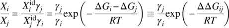
The solubility, , of a crystal form i in a solution can be presented as:

(22.1)

where

• is an ideal solubility.
• γ_i is an activity coefficient, which accounts for deviations from the ideal behavior in a mixture of liquid solute and solvent.
• ∆G_i is a free energy difference between the liquid and solid solute at the temperature of interest, T.
• R is the universal gas constant.

In case no additional phase transition takes place in the temperature range between the temperature of interest, T, and the melting point, T_m, the ∆G_i can be presented as

(22.2)

where

• ΔH_fus is the heat of fusion of the polymorph i at its melting point, T_m.
• ΔC_p is a difference between the heat capacities of the liquid and solid states of the form i, which is always positive.

For practical reasons, it is usually assumed that ΔC_p is constant and equal to one estimated at the T_m, ΔC_pm. In that case the free energy difference, ∆G_i, can be presented as:

(22.3)

However, as a rule, the ΔC_pm property is not available and further approximations should be taken. The most popular assumptions that are used in the literature are ΔC_pm = 0 (Assumption A) and ΔC_pm = ΔS_fus (Assumption B), where ΔS_fus is entropy of fusion at the melting point, ΔS_fus = ΔH_fus/T_m. Equation (22.3) is simplified upon these assumptions to Eqs. (22.4) and (22.5), respectively:

(22.4)

(22.5)

While the first assumption (A) is usually justified by negligibly low value of the ΔC_pm (which is not always true), the latter one (B) is based on the observation by Hildebrand and Scott that ln is linearly related to ln T [16].

In order to understand the errors introduced by both assumptions, they were mathematically derived below from Eq. (22.3) based on a first‐order Taylor expansion of ln(T_m/T) ≈ (T_m/T − 1), which is correct only in case of T_m/T close to 1 (Table 22.1).

Tm/Ta	ln(Tm/T)	Tm/T − 1b	Relative Error (%)b	2(Tm/T − 1)/(Tm/T + 1)c	Relative Error (%)c
1.1 (330/300)	0.095	0.1	4.9	0.095	−0.1
1.2 (360/300)	0.182	0.2	9.7	0.182	−0.3
1.3 (390/300)	0.262	0.3	14.3	0.261	−0.6
1.4 (420/300)	0.337	0.4	18.9	0.333	−0.9
1.5 (450/300)	0.406	0.5	23.3	0.400	−1.3
1.6 (480/300)	0.470	0.6	27.7	0.462	−1.8

^aExamples of T_m and T values in K are presented in the parentheses. T is chosen to be close to the room temperature.

^bFirst‐order Taylor series expansion: ln(T_m/T) ≈ (T_m/T − 1).

^cFirst‐order expansion adopted by Hoffman [17]: ln(T_m/T) ≈ 2(T_m/T − 1)/(T_m/T + 1). This expansion is significantly more accurate than the first‐order Taylor expansion.

22.3.1.1 Assumption A

Transformation of ln(T_m/T) to (T_m/T − 1) in the last term of Eq. (22.3) results in the complete cancelation of the last two terms of the equation:

Thus, the applied transformation is equivalent to neglecting the ΔC_pm term (ΔC_pm = 0, Eq. 22.4). Since at T < T_m, (T_m/T − 1) is always larger than ln(T_m/T) (Table 22.1), and ΔC_pm is always positive. Assumption A leads to the systematic overestimation of the ∆G_i, resulting into underestimation of the solubility relative to the predictions based on Eq. (22.3). The ∆G_i error introduced by Assumption A relative to Eq. (22.3) is related to the error of the first‐order Taylor series expansion and can be presented as

(22.6)

This error is proportional to the ΔC_pm property and increases with T_m/T due to an increasing inaccuracy in the first‐order Taylor expansion (Table 22.1).

22.3.1.2 Assumption B

In attempt to counterbalance the error introduced by the direct Taylor expansion transformation used in Assumption A, one may apply a reverse transformation, (T_m/T − 1) ≈ ln(T_m/T), to Eq. (22.4):

The result is equivalent to Eq. (22.5), which was derived under assumption of ΔC_pm = ΔS_fus. Since ΔH_fus (and ΔS_fus) is always positive and the error introduced by the reverse transformation is opposite to the one introduced by the direct transformation (Assumption A), a cancelation of errors should take place. The resulting ∆G_i error introduced by Assumption B relative to Eq. (22.3) is equal to

(22.7)

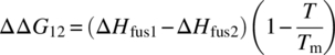
It is apparent from this equation that the error will change sign in case of ΔS_fus > ΔC_pm, resulting in underestimation of the ∆G_i and overestimation of solubility relative to the predictions based on Eq. (22.3). In the case where ΔS_fus is more than twice as large as ΔC_pm, an absolute error introduced by Assumption B will exceed the error introduced by Assumption A. This phenomenon may have resulted in the contradicting results of the relative accuracy of Assumptions A and B in the literature [18–21]. It was shown recently [22] that a relation between ΔS_fus and ΔC_pm properties is dependent on a chemical class of organic compounds. A ratio of the absolute ∆G_i errors introduced by Assumptions B (Eq. 22.7) and A (Eq. 22.6), , is presented for 68 organic compounds in Figure 22.1. Only 12 non drug‐like compounds out of 68 totally displayed a relative error of more than 1, indicating that Assumption B introduces a higher absolute error than Assumption A. A majority of these compounds can be characterized by the low value of their differential heat capacities, ΔC_pm < 40 J/mol/K (Figure 22.1). All of these considerations provide justification for the application of Assumption B over Assumption A for drug‐like compounds.

22.3.1.3 Assumption C

Another valuable approximation of Eq. (22.2) was proposed by Hoffman [17] based on a significantly more accurate series expansion of ln(T_m/T) than the first‐order Taylor expansion applied above (Table 22.1):

(22.8)

The differential heat capacity, ΔC_p, is assumed to be both not negligible and independent on temperature. The lack of significant errors introduced by the ln(T_m/T) expansion, and perhaps a more justified approximation for the ΔC_p, makes Assumption C a generally more thermodynamically sound model than Assumptions A and B. Additionally, Eq. (22.8) can be seen as equivalent to Eq. (22.4) (Assumption A) scaled down by a factor of T/T_m. This effectively introduces a correction for the overestimation of the ∆G_i by Assumption A.

22.3.2 Comparison of the Assumptions

A rigorous comparison of Assumptions A, B, and C is complicated by the fact that the differential heat capacity in Eq. (22.2) is temperature dependent and for the general case increases as temperatures decrease [19, 21, 25]. Even for the cases when the ΔC_p at the melting point is known, Eq. (22.3) might not produce a reliable reference for comparison. An accurate temperature dependence of the heat capacities of both solid and liquid states in a polynomial form, C_p = A₀ + A₁T + A₂T², has limited data available in the literature [21, 23, 26]. Applicability of such a model depends on the reliability of an extrapolation of the observed temperature behavior of the heat capacities above (liquid state) and below (solid state, supercooled liquid) T_m at the temperature of interest. The difference between the coefficients (A_i) of the liquid and solid forms reflects a temperature dependence of the differential heat capacity. In such a case, the free energy difference between the liquid and solid solutes can be presented as

(22.9)

where

• ΔA_i = A_i (liquid) − A_i (solid).

In Table 22.2 ∆G_i predictions at room temperature using Eq. (22.3) and Assumptions A, B, and C are compared to the results based on Eq. (22.9). The differential heat capacities of all the compounds increase significantly at room temperature relative to the values at their melting points (Table 22.2). The temperature dependence of the ΔC_p leads to a decrease of the predicted ∆G_i values at the room temperature relative to the predictions based on the differential heat capacities at T_m (Eq. 22.3). A resulting mean absolute error (MAE) of Eq. (22.3) predictions is 1.0 kJ/mol (Table 22.2). This ∆G_i error corresponds to an average underestimation of the ideal solubilities at room temperature by 33%. The MAE values of the ∆G_i predictions based on Assumptions A, B, and C for the same compounds relative to results obtained by Eq. (22.9) are 3.9, 1.9, and 0.4 kJ/mol, respectively. The corresponding errors of the ideal solubility predictions at the room temperature are 79, 54, and 15%, respectively. Thus, the presented results demonstrate that the Hoffman approximation significantly outperforms Assumptions A and B. The largest error of ideal solubility prediction at ambient temperature is made using Assumption A, which introduces a large ∆G_i error.

					Error Relative to Eq. (22.9) (kJ/mol)
Name	Tm (K)	ΔHfus (kJ/mol)	ΔCpm (J/[mol K])	ΔCp (T = 298.2 K) (J/[mol K])	Eq. (22.3)	Eq. (22.4)	Eq. (22.5)	Eq. (22.8)
Carbamazepine I [23]	463.7	26.3	109.8	164.6	0.7	4.4	2.5	1.0
Carbamazepine III [23]	452.4	27.2	111.3	184.3	1.0	4.3	2.5	1.1
Paracetamol [26]	442.2	28.1	99.6	165.8	0.6	3.3	1.6	0.3
Anisic acid [21]	455.4	27.8	81.4	150.6	0.8	3.3	1.4	0.0
Diethylstilbestrol [21]	441.8	28.8	43.8	262.3	2.0	3.2	1.5	0.2
Mannitol [21]	438.7	50.6	163.8	290.3	1.1	5.3	2.4	0.1
Naproxen [21]	428.5	31.5	108.6	220.3	0.9	3.3	1.7	0.4
MAEb (kJ/mol)					1.0	3.9	1.9	0.4

^aThe ΔA₂ term (Eq. 22.9) is different from zero only in the case of carbamazepine.

^bMean absolute error is calculated as an arithmetic average of the absolute errors of the predictions performed by the corresponding approach.

22.3.3 Application to Polymorphs Solubility Ratio

The solubility ratio of polymorphs can be presented by Eq. (22.10), and seems to be an optimal test for validation of the different ∆G_i models considered in Section 22.3.1:

(22.10)

Recently, evaluations of different models for polymorph solubility ratio prediction based on thermal properties of the polymorphs were reported [11, 12]. Pudipeddi and Serajuddin have found that for 10 polymorphic pairs of predictions based on Assumption C were “slightly closer” to the experimental data than the results obtained by Assumption A [11]. Mao et al. have considered calculations based on Assumption A [12]. A validation of this approach on nine polymorphic systems led to the conclusion that the utilization of Assumption A typically leads to an error of only 10% or less. An obvious drawback of these two studies is that the very limited data sets of the polymorph pairs were adopted for the testing of only selected assumptions. Therefore, to increase statistical significance of the results, further side‐by‐side verification of all three assumptions using larger experimental data sets could prove to be very important.

Two different data sets were selected for the model validation in this study, which contains 10 monotropically related (Table 22.3) and 18 enantiotropically related (Table 22.4) pairs of nonsolvated polymorphs. Each data point in these sets contains information on experimental properties such as solubility, X_i, melting point, T_m, and heats of fusion, ΔH_fus. The following considerations were taken into account during the data selection. There is quite a common misperception that the polymorph solubility ratio is solvent independent. However, according to Eq. (22.10), this is only true when the activity coefficients for the two polymorphs are identical to each other in any solvent [12, 47]. This takes place in the case of an infinite solubility limit (dilute solution). In such a case, each polymorph in the liquid state is not a significant part of the solvent system in which the actual solubility is measured. Thus, whenever possible, solubility data was chosen for polymorphs approximately tens of mg/ml or less. Moreover, at these low concentrations, there is no need to convert mg/ml or μg/ml units to mol fractions, in which Eq. (22.10) is presented. One drawback of the selection of very low solubility data is a higher standard deviation of the experimental polymorph solubility ratios (Appendix 22.A).

Compound	Tm1 (K)	∆Hfus1 (kJ/mol)	Tm2 (K)	∆Hfus2 (kJ/mol)	T (K)	S1/S2, exp	Assumption A	Assumption B	Assumption C	Eq. (22.13)	Eq. (22.14)	Eq. (22.15)	Eq. (22.16)
Chloramphenicol palmitate (A/B) [24, 27]	362	41.9	368	64.1	303	4.2	5.95	4.93	4.19	5.14	4.74	4.10	3.60
Tolbutamide (I/III) [24, 28]	379	18.5	400	24.5	303	1.22	2.42	2.08	1.84	1.29	1.78	1.65	1.55
Ritonavir (I/II) [9]	395.2	56.4	398.2	63.3	298	2.39a	2.29	2.01	1.80	2.17	2.02	1.83	1.69
MK571(II/I) [29]	425.2	49.0	437.2	54.0	309	1.64	2.59	2.08	1.77	1.56	1.77	1.61	1.50
Cyclopenthiazide (II/I) [30]b	496.2	98.42	512.5	105.5	310	1.78	6.32	3.40	2.30	1.72	2.96	2.31	1.93
E2101 (II/I) [31]	413.0	35.2	421.3	38.2	298	1.25	1.74	1.54	1.40	1.32	1.43	1.35	1.28
Indomethacin (α/γ) [15]	429.2	36.14	435.2	36.49	318	1.1	1.19	1.14	1.10	1.11	1.04	1.03	1.03
Acemetacin (II/I) [3]	423.2	48.4	423.7	50.7	293	1.67	1.36	1.29	1.23	1.52	1.34	1.27	1.22
Torasemide (II/I) [32]	430.2	29	434.7	37.2	293	2.74	3.26	2.58	2.16	2.51	3.00	2.45	2.10
Cimetidine (A/B) [33, 34]	413.5	44.03	413.7	44.08	298	1.15	1.01	1.01	1.01	1.21	1.01	1.00	1.00
MAE							1.01	0.50	0.32	0.19	0.38	0.27	0.33

Results of application of Eqs. (22.14)–(22.16) adopting T_m = T_m2 are presented. The explicit equations for solubility ratio predictions are presented in Appendix 22.B.

^aPolymorph solubility data in ethyl acetate:heptanes 2 : 1 mixture is adopted for solubility ratio estimation.

^bAn enantiotropic relationship between forms I and II with a very low transition temperature was proposed in the literature [14].

Compound	Tm1 (K)	∆Hfus1 (kJ/mol)	Tm2 (K)	∆Hfus2 (kJ/mol)	T (K)	S1/S2, exp	Assumption A	Assumption B	Assumption C	Eq. (22.14)	Eq. (22.15)	Eq. (22.16)
Axitinib (IV/VI) [35–37]	491.90	47.15	484.80	51.79	310	1.25	1.62	1.53	1.45	1.91	1.67	1.51
Axitinib (IV/XXV) [35–37]	491.90	47.15	490.40	50.43	310	1.25	1.54	1.42	1.33	1.60	1.45	1.34
Paracetamol (II/I) [24, 38]	429	26.9	442	28.1	303	1.3	1.45	1.30	1.21	1.16	1.13	1.11
Buspirone‐HCL (II/I) [39]	476.8	42.24	463.0	47.45	303	1.7	1.49	1.49	1.46	2.04	1.78	1.60
Carbamazepine (I/III) [40]	462	26.4	448	29.3	299.2	1.20	1.19	1.21	1.21	1.47	1.37	1.30
F2692 [24]	453	27.17	445	29.32	303	1.8	1.15	1.16	1.15	1.31	1.25	1.20
Gepirone hydrochloride (II/I) [41]	485	41.6	453	47.1	303	2.01	0.99	1.19	1.31	2.06	1.80	1.62
Indiplona	465.51	41.63	463.08	45.89	298	1.1	1.74	1.58	1.46	1.85	1.63	1.48
Nimodipine (I/II) [3]	397.2	39	389.2	46	298	2	1.52	1.49	1.46	1.94	1.78	1.66
Phenylbutazone (II/III) [24]	370	21.9	368	24.4	303	1.1	1.15	1.14	1.13	1.19	1.17	1.16
Piroxicam (I/II) [42]	475.8	36.54	472.9	37.43	310	0.99	1.06	1.07	1.06	1.13	1.10	1.08
Propranolol hydrochloride (I/II) [43]	436.2	31.35	435.0	36.62	293	1.34	1.98	1.75	1.60	2.03	1.78	1.61
Retinoic acid (II/I) [44]	456.3	36.8	456.9	37.1	310	1.32	1.05	1.04	1.03	1.04	1.03	1.03
RG12525 (II/I) [45]	431.0	43.10	427.8	46.86	304	1.26	1.41	1.35	1.31	1.54	1.43	1.36
Sulfathiazole (I/III) [24]	474.2	27.75	446.8	29.47	303	1.68	0.81	0.93	1.01	1.25	1.20	1.16
WIN63843 (I/III) [46]	337.7	28.87	334.4	31.88	296	1.04	1.04	1.04	1.05	1.15	1.14	1.13
Cimetidine (C/B) [33, 34]	417.5	43.13	413.7	44.08	298	1.23	0.99	1.01	1.03	1.11	1.09	1.08
Cimetidine (C/A) [33, 34]	417.5	43.13	413.5	44.03	298	1.07	0.98	1.01	1.02	1.11	1.09	1.08
MAE							0.34	0.28	0.25	0.29	0.24	0.22

Results of application of Eqs. (22.14)–(22.16) adopting T_m = T_m2 are presented. The explicit equations for solubility ratio predictions are presented in Appendix 22.B.

^aCollman B, private communication.

22.3.3.1 Monotropic Case

The initial validation of the solubility ratio models was performed using monotropically related polymorphs. In the following discussions notation 1 and 2 will refer to the higher and lower soluble polymorphs. Equations used for the solubility ratio predictions in this section are explicitly listed in Appendix 22.B. Given that low solubility experimental data was selected for the test, it seems reasonable to expect that cancelation will take place not only between the activity coefficients of both polymorphs in the solution but also between the errors introduced by the ∆G_i assumptions. Results of the relative solubility predictions utilizing Assumptions A, B, and C (Appendix 22.B) for each polymorph are presented in Table 22.3. The corresponding MAE values relative to the experimental X₁/X₂ observations are 1.01, 0.50, and 0.32, respectively. These observations disagree with previous reports that Assumption A results in an error of only 10% or less [12] and that Assumption C is just slightly closer to the experimental data than the results obtained by Assumption A [11]. The obtained MAE values demonstrate that a complete cancelation of errors does not take place and, as a result, Assumption C remains significantly more accurate than the others. According to the error analysis presented in Section 22.3.1 (Eqs. 22.6 and 22.7), the lack of error cancelation in the ΔΔG₁₂ prediction can be accounted for by non‐negligible differences of the ΔC_pm ([ΔC_pm − ΔS_fus] in case of Assumption B) and/or T_m properties between the two polymorphs. For example, in case of Assumption A, the error of the ΔΔG₁₂ prediction relative to the one based on Eq. (22.3) can be presented as a difference of errors (Eq. 22.6) between two polymorphs:

(22.11)

The following two limiting cases can be derived from Eq. (22.11). In the case of relatively insignificant variations of the ΔC_pm terms, the ΔΔG_error is proportional to T{[(T_m1/T − 1) – ln(T_m1/T)] – [(T_m2/T − 1) – ln(T_m2/T)]}. In the case where variations of ΔC_pm are noticeably more significant than the variations of Τ_m, the ΔΔG_error is proportional to (ΔC_pm1 − ΔC_pm2). The ΔC_pm values should be replaced by the (ΔC_pm − ΔS_fus) differences for the error estimation of the ΔΔG₁₂ prediction based on Assumption B.

It is easy to show from Eq. (22.10) that for dilute solutions, the difference between the natural logarithms of polymorph solubility ratios as predicted by Assumption A or B and Eq. (22.3) should be proportional to the ΔΔG_error:

(22.12)

According to Eq. (22.11) in case of Assumption A, this difference will be equal to {ΔC_pm2[(T_m2/T − 1) – ln(T_m2/T)] – ΔC_pm1[(T_m1/T − 1) – ln(T_m1/T)]}/R. It is reasonable to propose that the difference between natural logarithms of polymorph solubility ratios as predicted by Assumption A or B, and those observed experimentally, may be described by the similar factors as presented in Eqs. (22.11) and (22.12). In the absence of the ΔC_pm values, a correlation was tested between the ln(X₁/X₂) − ln(X₁/X₂)_exp predictions based on the different assumptions and {[(T_m2/T − 1) – ln(T_m2/T)] – [(T_m1/T − 1) – ln(T_m1/T)]} property (Figure 22.2). High linear correlation coefficients, R², of 0.92 and 0.91 were found for the predictions based on Assumptions A and B, respectively (Figure 22.2a and b). This observation suggests a higher and a more systematic contribution to the ΔΔG_error by the differences in the T_m values, rather than by the differences in the ΔC_pm or (ΔC_pm − ΔS_fus) properties. A noticeably weaker correlation (having an R² of 0.72) (Figure 22.2c) was observed for the predictions based on Assumption C.

Found simple linear regressions (Figure 22.2) can be used for estimations of likely errors in the solubility ratio predictions of monotropically related polymorphs based on the different assumptions. The MAE values of the prediction (0.24, 0.22, and 0.19, respectively) are based on Assumptions A, C, and B after the errors are corrected by using simple functions of the melting points. The latter result corresponds to the best agreement with the experimental observations using the approaches presented in Table 22.3. This suggests that the polymorph solubility ratio of the monotropically related polymorphs can be best predicted through the following relationship:

(22.13)

Based on the above observation of the high contribution to the ΔΔG_error by the differences in the T_m values, an alternative approach can be suggested. In order to better counterbalance the prediction errors, it was proposed to adopt a single T_m value for both polymorphs used in the solubility ratio predictions. In this case, an improvement of the predictions should take place through the increase of ΔG₁ (T_m = T_m2) or the decrease of ΔG₂ (T_m = T_m1). The following simplifications of the ΔΔG₁₂ calculation based on Assumptions A, B, and C are proposed:

(22.14)

(22.15)

(22.16)

Besides a possible improvement of the polymorph solubility prediction, the proposed equations more importantly depend on only two input parameters: T_m of one of the forms and a difference between the enthalpies of fusion of the two polymorphs. This fact makes these equations useful for solving one of the major objectives of the current study – the development of a working equation for the estimation of the potential impact of an unknown and more stable form on drug solubility.

The application of Eqs. (22.14)–(22.16) in predicting the solubility ratio of monotropically related polymorphs adopting T_m = T_m2 is presented in Table 22.3. Eqs. (22.14) and (22.15) dramatically improve agreement with the experimental data. The MAE drops from 1.01 to 0.38 for Assumption A using Eq. (22.14). In the case of Assumption B, the MAE changes from 0.50 to 0.27 using Eq. (22.15). No improvement was found for Assumption C, in which the MAE value practically does not change when adopting Eq. (22.16) with a single T_m value of T_m2. When T_m = T_m1, the MAE values for Eqs. (22.14)–(22.16) are 0.28, 0.29, and 0.35, respectively. This demonstrates behavior of the X₁/X₂ predictions similar to those found with T_m = T_m2.

22.3.3.2 Enantiotropic Case

A thermodynamic expression of the solubility ratio of enantiotropically related polymorphs requires knowledge of the temperature and enthalpy of the solid–solid transition [12], which is often difficult to measure accurately. For this reason, only enantiotropic systems with available melting properties for both polymorphs were included in this study. Results of the application of Assumptions A, B, and C to the predictions of the solubility ratio of the enantiotropically related polymorphs are presented in Table 22.4. An overall accuracy of the predictions is noticeably better than it was found for the monotropic system (Table 22.3). As in the monotropic case, the agreement with the experimental data is worse for the calculations based on Assumption A (MAE value is 0.34), relative to those based on Assumptions B and C (MAE values are 0.28 and 0.25, respectively).

No strong correlation was found between the ln(X₁/X₂) − ln(X₁/X₂)_exp values and the {[(T_m2/T − 1) – ln(T_m2/T)] – [(T_m1/T − 1) – ln(T_m1/T)]} property in case of enantiotropic system based on the different assumptions. Thus, error correction similar to that proposed by Eq. (22.13) is not applicable to the enantiotropic case. However, an improvement of the predictions based on Assumptions A, B, and C is possible by the application of Eqs. (22.14)–(22.16), respectively (Table 22.4). The best performance was found for Eq. (22.16) and Eq. (22.15), both resulting in MAE values of 0.22 and 0.24 (where T_m = T_m2 or T_m1), respectively.

It should be noted that Eqs. (22.14)–(22.16) cannot describe the change of the relative stability of the enantiotropically related polymorphs with temperature. To do so would result in the ΔΔG₁₂ property having the wrong sign above the solid–solid transition, T_t (ΔΔG₁₂(T_t) = 0). Thus, the application of these equations to enantiotropic polymorphs is limited to systems with temperatures below T_t.

From the above considerations, which are based on the analysis of the largest reported experimental data set of both monotropic and enantiotropic systems, an application of the original (Eq. 22.8) (Appendix 22.B) and modified (Eq. 22.16) Hoffman approaches as well as of Eq. (22.15) are recommended for an accurate solubility ratio prediction for both monotropic and enantiotropic polymorphic systems. Since the latter two approaches utilize the melting temperature measurements of only one form, T_m2 or T_m1, they can be used in combination with the statistical analysis of the differences of the heat of fusions of polymorphs, for an estimation of the potential impact of an unknown and more stable form on drug solubilities (see Section 22.4 for more details).

22.4 APPLICATION TO AN ESTIMATION OF LIKELY IMPACT ON DRUG SOLUBILITY BY UNKNOWN MORE STABLE FORM

Below we present two approaches to predict a likely change of drug solubility due the form change. The first thermal data approach is based on a combination of statistical analysis of the experimental heat of fusion differences between polymorphic pairs and the proposed in the current work Eq. (22.16) for the ideal solubility ratio prediction. The second, solubility ratio approach is based on statistical results from experimental solubility ratio observations.

22.4.1 Thermal Data Approach

This approach is based on application of the modified Hoffman Eq. (22.16) coupled with statistical analysis of experimentally determined heat of fusion differences between polymorphs. The ideal solubility ratio predictions can be carried out for a known form with available melting temperature and likely changes in heat of fusion, ΔΔH_fus. In order to do that, a survey of thermal data for 101 polymorphic pairs was carried out, where most of the data where found in one literature source [24] and the rest were taken from Tables 22.3 and 22.4 of the current study. Trends in heat of fusion changes between polymorphs were presented in the form of the cumulative relative frequency distribution in Figure 22.3. The cumulative relative frequency distribution is particularly useful for describing the likelihood that a variable (heat of fusion difference) will not exceed a certain value. It was found that there is a 50% probability that the change in heat of fusion for a polymorphic pair is less than or equal to 3.0 kJ/mol (Figure 22.3). The probability of heat of fusion difference between a pair of polymorphs not exceeding values of 6.2 and 16.7 kJ/mol is, respectively, 80 and 95%. Combining these ΔΔH_fus values with Eq. (22.16) allows estimation at the different probability levels of maximum impact on ideal solubility by a new and more stable polymorph. Though the thermal data approach relies on the statistical analysis (of ΔΔH_fus), it introduces some degree of the dependence on the thermal properties (T_m) of the reference form through Eq. (22.16). Therefore predictions based on this method are form specific.

22.4.2 Solubility Ratio Approach

An alternative approach is based on the statistical analysis of the polymorph solubility ratio observations. A survey of solubility changes for 153 polymorphic pairs was carried out, where most of the data were found in open literature sources [11] and some were extracted from in‐house Pfizer data or provided by company‐associated institutions. A statistical analysis of the experimental data was performed on the basis of cumulative relative frequency distribution, presented in Figure 22.4. It was found that there is a 50% probability that the change in solubility is less than 1.2‐fold for a polymorphic switch (Figure 22.3). The probability of the solubility ratio between a pair of polymorphs not exceeding value of 1.5 is 80%. It was also shown that only in 5% of the studied cases the change in solubility for polymorphic pairs would be more than twofold (Figure 22.4).

The presented trend of probabilities of the relative solubility changes is purely statistical and does not provide any direct dependence on thermal data of the current form. Therefore this approach may be considered as form nonspecific one. In addition, majority of the solubility ratio measurements are performed at different temperatures in the range of 20–40 °C [11], rather than at the room temperature. That may introduce some level of noise in the predictions based on this method.

22.4.2.1 Qualification/Quantification of Impact of Likely Form Change on Drug Absorption

A significant solubility difference between two polymorphs can result in difference in oral absorption and may affect bioavailability [48]. Orally administrated immediate‐release drug products are categorized in the Biopharmaceutics Classification System (BCS) according to their aqueous solubility and permeability [49]. These properties together with dissolution rate control drug absorption. Absolute bioavailability of a drug is also affected by first‐pass intestinal and hepatic metabolism [50]. It is reasonable to assume that polymorphic forms of a particular compound should display similar permeabilities and first‐pass clearances. Therefore, the differences in fraction absorbed and absolute bioavailability between oral products (based on different polymorphs) are controlled by solubility and dissolution rate. This assumes that the polymorph interaction with excipients is negligible. While the dissolution rate can be generally controlled by changing the particle size, a thermodynamic aqueous solubility is a fundamental property of the polymorphic form that cannot be modified.

The classification of drug form solubility is based on dimensionless dose number D₀, which is a function of maximum dose strength D (mg) and solubility S (mg/ml):

(22.17)

Here V₀ is volume of water taken with the dose, which is generally set to 250 ml. Solid forms of drugs with D₀ equal to or less than 1 are considered being highly soluble [51]. According to the BCS system, such forms are characterized as classes I and III. An estimation of a likely change in solubility due to transformation to a new and more stable form allows prediction of the potential impact on D₀ that a new form could present. The potential risk associated with the late discovery of a new stable form can be accessed based on a degree of probability of solubility (and D₀) change, as discussed above, and projected change of drug absorption. A qualitative analysis of the impact of form change on absorption can be based on the BCS system; here we classify risk as associated with a potential change of the drug class from I to II or from III to IV. In addition, computational simulations (e.g. GastroPlus, Simulations Plus, Inc., Lancaster, CA) may be adopted for a (semi‐)quantitative analysis of sensitivity of drug absorption to a potential form change.

22.5 CONCLUSION

One of the main purposes of this study is to develop valid methods for the estimation of a potential impact of an unknown and more stable form on drug solubility. This information has a crucial practical application in the pharmaceutical industry by supporting the risk assessment of an API solid form selection for commercial development of an oral drug. Two independent approaches to predict a likely change of drug solubility due the form change were suggested in the current study. One of them is based on the modified Hoffman Eq. (22.16), which was found through a consistent theoretical consideration of the errors introduced by the different popular assumptions used for absolute and relative polymorph solubility predictions.

In addition, the first side‐by‐side validation of all three popular assumptions for the relative polymorph solubility prediction was performed on the largest up‐to‐date experimental data set. It was demonstrated that Assumption A (ΔC_pm = 0) results in noticeable errors that significantly exceed the previously reported values of 10% or less [12]. Based on the current study, this assumption is not recommended for the polymorph solubility ratio prediction of drug‐like molecules, especially in case of the monotropically related systems. The superiority of Assumption C (Hoffman equation) over the other assumptions, and in particular over Assumption A, was found to be much stronger than was previously reported [11]. Assumption B (ΔC_pm = ΔS_fus) demonstrated an intermediate performance between Assumptions A and C.

Finally, based on the error analysis, a new model, Eq. (22.13), was proposed for the solubility ratio prediction of the monotropically related polymorphs. This model provided the best agreement with the experimental data set of 10 polymorphic pairs.

22.A PROPAGATION OF ERRORS OF THE SOLUBILITY RATIO MEASUREMENTS

Assuming independence of the solubility measurements of two polymorphs, X₁ and X₂, the standard deviation of the solubility ratio, k = X₁/X₂, can be expressed as [52]:

(22.A.1)

In case σ(X₁) ≈ σ(X₂) = σ(X), the following resulting equation can be obtained:

(22.A.2)

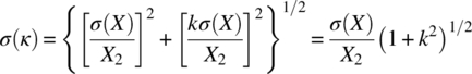
Equation (22.A.2) demonstrates that the error of the solubility ratio measurements increases with the increase of the k value and with the decrease of the polymorph solubility, X₂. For example, for the solubility X₂ of 0.2 μg/ml, σ(X) equal to 0.02 μg/ml, and k value of 2, the σ(k) is equal to 0.22.

22.B SUMMARY OF EXPLICIT EQUATIONS USED FOR THE SOLUBILITY RATIO PREDICTIONS

ACKNOWLEDGMENTS

The authors would like to thank Mr. Brian Samas, Dr. Neil Feeder, Dr. Paul Meenan, Dr. Robert Docherty and Dr. Bruno Hancock for the valuable comments and discussions. The authors also wish to thank Mr. Anthony M. Campeta for providing the experimental thermal and solubility data on the axitinib polymorphs. YAA is thankful to Mr. Brian D. Bissett for a thorough review of the manuscript.

REFERENCES

1. 1. Brittain, H.G. (ed.) (1999). Polymorphism in Pharmaceutical Solids. New York: Marcel Dekker.
2. 2. Burger, A. and Ramberger, R. (1979). On the polymorphism of pharmaceuticals and other organic molecular crystals. I: theory of thermodynamic rules. Mikrochim. Acta II: 259–271.
3. 3. Grunenberg, A., Henck, J.‐O., and Siesler, H.W. (1996). Theoretical derivation and practical application of energy/temperature diagrams as an instrument in preformulation studies of polymorphic drug substances. Int. J. Pharm. 129: 147–158.
4. 4. Byrn, S., Pfeiffer, R., Ganey, M. et al. (1995). Pharmaceutical solids: strategic approach to regulatory considerations. Pharm. Res. 12: 945–954.
5. 5. Yu, L.X., Furness, M.S., Raw, A. et al. (2003). Scientific considerations of pharmaceutical solid polymorphs in abbreviated new drug applications. Pharm. Res. 20: 531–536.
6. 6. Brittain, H.G. and Grant, D.J.W. (1999). Effects of polymorphism and solid‐state solvation on solubility and dissolution rate. In: Polymorphism in Pharmaceutical Solids (ed. H.G. Brittain), 279–330. New York: Marcel Dekker.
7. 7. Kempf, D.J., Marsh, K.C., Denissen, J.F. et al. (1995). ABT‐538 is a potent inhibitor of human immunodeficiency virus protease and has high oral bioavailability in humans. Proc. Natl. Acad. Sci. U. S. A. 92: 2484–2488.
8. 8. Bauer, J., Spanton, S., Henry, R. et al. (2001). Ritonavir: an extraordinary example of conformational polymorphism. Pharm. Res. 18: 859–866.
9. 9. Chemburkar, S.R., Bauer, J., Deming, K. et al. (2000). Dealing with the impact of ritonavir polymorphs on the late stages of bulk drug process development. Org. Process Res. Dev. 4: 413–417.
10. 10. Morissette, S.L., Soukasene, S., Levinson, D. et al. (2003). Elucidation of crystal form diversity of the HIV protease inhibitor ritonavir by high‐throughput crystallization. Proc. Natl. Acad. Sci. U. S. A. 100: 2180–2184.
11. 11. Pudipeddi, M. and Serajuddin, A.T.M. (2005). Trends in solubility of polymorphs. J. Pharm. Sci. 94: 929–939.
12. 12. Mao, C., Pinal, R., and Morris, K.R. (2005). A quantitative model to evaluate solubility of polymorphs from their thermodynamic properties. Pharm. Res. 22: 1149–1157.
13. 13. Grant, D.J.W. and Higuchi, T.T. (1990). Solubility Behavior of Organic Compounds. New York: Wiley.
14. 14. Gu, C.‐H. and Grant, D.J.W. (2001). Estimating the relative stability of polymorphs and hydrates from heats of solution and solubility data. J. Pharm. Sci. 90: 1277–1287.
15. 15. Hancock, B.C. and Parks, M. (2000). What is the true solubility advantage for amorphous pharmaceuticals? Pharm. Res. 17: 397–403.
16. 16. Hildebrand, J.H. and Scott, R.L. (1962). Regular Solutions. Englewood Cliffs, NJ: Prentice‐Hall.
17. 17. Hoffman, J.D. (1958). Thermodynamic driving force in nucleation and growth processes. J. Chem. Phys. 29: 1192–1193.
18. 18. Mishra, D.S. and Yalkowsky, S.H. (1992). Ideal solubility of a solid solute: effect of heat capacity assumptions. Pharm. Res. 9: 958–959.
19. 19. Neau, S.H. and Flynn, G.L. (1990). Solid and liquid heat capacities of n‐alkyl para‐aminobenzoates near the melting point. Pharm. Res. 7: 1157–1162.
20. 20. Neau, S.H., Flynn, G.L., and Yalkowsky, S.H. (1989). The influence of heat capacity assumptions on the estimation of solubility parameters from solubility data. Int. J. Pharm. 49: 223–229.
21. 21. Neau, S.H., Bhandarkar, S.V., and Hellmuth, E.W. (1997). Differential molar heat capacity to test ideal solubility estimations. Pharm. Res. 14: 601–605.
22. 22. Pappa, G.D., Voutsas, E.C., Magoulas, K., and Tassios, D.P. (2005). Estimation of the differential molar heat capacities of organic compounds at their melting point. Ind. Eng. Chem. Res. 44: 3799–3806.
23. 23. Defossemont, G., Randzio, S.L., and Legendre, B. (2004). Contributions of calorimetry for C_p determination and of scanning transitiometry for the study of polymorphism. Cryst. Grow. Des. 4: 1169–1174.
24. 24. Yu, L. (1995). Inferring thermodynamic stability relationship of polymorphs from melting data. J. Pharm. Sci. 84: 966–974.
25. 25. Gracin, S., Brinck, T., and Rasmuson, A.C. (2002). Prediction of solubility of solid organic compounds in solvents by UNIFAC. Ind. Eng. Chem. Res. 41: 5114–5124.
26. 26. Hojjati, H. and Rohani, S. (2006). Measurement and prediction of solubility of paracetamol in water−isopropanol solution. Part 2. Prediction. Org. Process Res. Dev. 10: 1110–1118.
27. 27. Aguiar, A.J., Krc, J. Jr., Kinkel, A.W., and Samyn, J.C. (1967). Effect of polymorphism on the absorption of chloramphenicol from chloramphenicol palmitate. J. Pharm. Sci. 56: 847–853.
28. 28. Rowe, E.L. and Anderson, B.D. (1984). Thermodynamic studies of tolbutamide polymorphs. J. Pharm. Sci. 73: 1673–1675.
29. 29. Ghodbane, S. and McCauley, J.A. (1990). Study of the polymorphism of 3‐((3‐(2‐(7‐chloro‐2‐quinolinyl)‐(E)‐ethenyl)phenyl)((3‐(dimethylamino‐3‐oxopropyl)thio)methyl)‐thio)propanoic acid (MK571) by DSC, TG, XRPD and solubility measurements. Int. J. Pharm. 59: 281–286.
30. 30. Gerber, J.J., vander Watt, J.G., and Lötter, A.P. (1991). Physical characterization of solid forms of cyclopenthiazide. Int. J. Pharm. 73: 137–145.
31. 31. Kushida, I. and Ashizawa, K. (2002). Solid state characterization of E2101, a novel antispastic drug. J. Pharm. Sci. 91: 2193–2202.
32. 32. Rollinger, J.M., Gstrein, E.M., and Burger, A. (2002). Crystal forms of torasemide: new insights. Eur. J. Pharm. Biopharm. 53: 75–86.
33. 33. Shibata, M., Kokubo, H., Morimoto, K. et al. (1983). X‐ray structural studies and physicochemical properties of cimetidine polymorphs. J. Pharm. Sci. 72: 1436–1442.
34. 34. Crafts, P.A. (2007). The role of solubility modelling and crystallization in the design of active pharmaceutical ingredients. In: Chemical Product Design: Toward a Perspective Through Case Studies (ed. K.M. Ng, R. Gani and K. Dam‐Johansen), 23–85. Dordrecht, The Netherlands: Elsevier.
35. 35. Ye, Q., Hart, R.M., Kania, R. et al. (2006). Polymorphic forms of 6‐[2‐((methylcarbomoyl)phenylsulfanyl]‐3‐E‐[2‐(pyridin‐2‐yl)ethenyl]indazole. US Patent 0094763.
36. 36. Campeta, A.M., Chekal, B.P., McLaughlin, R.W., and Singer, R.A. (2008). Novel crystalline forms of a VEGF‐R inhibitor. PCT Int. Appl. WO 2008122858.
37. 37. Chekal, B., Campeta, A., Abramov, Y.A. et al. (2009). Facing the challenges of developing an API crystallization process for a complex polymorphic and highly‐solvating system. Part I. Org. Process Res. Dev. 13: 1327–1337.
38. 38. Sohn, Y.T. (1990). Study on the polymorphism of acetaminophen. J. Korean Pharm. Sci. 20: 97–104.
39. 39. Sheikhzadeh, M., Rohani, S., Traffish, M., and Murad, S. (2007). Solubility analysis of buspirone hydrochloride polymorphs: measurements and prediction. Int. J. Pharm. 338: 55–63.
40. 40. Behme, R.L. and Brooke, D. (1990). Heat of fusion measurement of a low melting polymorph of carbamazepine that undergoes multiple‐phase changes during differential scanning calorimetry analysis. J. Pharm. Sci. 80: 986–990.
41. 41. Behme, R.J., Brooke, D., Farney, R.F., and Kensler, T.T. (1985). Research article characterization of polymorphism of gepirone hydrochloride. J. Pharm. Sci. 74: 1041–1046.
42. 42. Vrečer, F., Vrbinc, M., and Meden, A. (2003). Characterization of piroxicam crystal modifications. Int. J. Pharm. 256 (256): 3–15.
43. 43. Bartolomei, M., Bertocchi, P., Ramusino, M.C. et al. (1999). Physico‐chemical characterization of the modifications I and II of (R, S) propranolol hydrochloride: solubility and dissolution. J. Pharm. Biomed. Anal. 21: 299–309.
44. 44. Caviglioli, C., Pani, M., Gatti, P. et al. (2006). Study of retinoic acid polymorphism. J. Pharm. Sci. 95: 2207–2221.
45. 45. Carlton, R.A., Difeo, T.J., Powner, T.H. et al. Preparation and characterization of polymorphs for an LTD₄ antagonist, RG 12525. J. Pharm. Sci. 85: 461–467.
46. 46. Rocco, W.L. and Swanson, J.R. (1995). WIN 63843 polymorphs: prediction of enantiotropy. Int. J. Pharm. 117: 231–236.
47. 47. Higuchi, W.I., Lau, P.K., Higuchi, T., and Shell, J.W. (1963). Solubility relationship in the methylprednisolone system. J. Pharm. Sci. 52: 150–153.
48. 48. Singhal, D. and Curatolo, W. (2004). Drug polymorphism and dosage form design: a practical perspective. Adv. Drug Deliv. Rev. 56: 335–347.
49. 49. Amidon, G.L., Lennernas, H., Shah, V.P., and Crison, J.R.A. (1995). Theoretical basis for a biopharmaceutic drug classification: the correlation of in vitro drug product dissolution and in vivo bioavailability. Pharm. Res. 12: 413–420.
50. 50. Varma, M.V.S., Obach, R.S., Rotter, C. et al. (2010). Physicochemical space for optimum oral bioavailability: contribution of human intestinal absorption and first‐pass elimination. J. Med. Chem. 53: 1098–1108.
51. 51. Kasim, N.A., Whitehouse, M., Ramachandran, C. et al. (2004). Molecular properties of WHO essential drugs and provisional biopharmaceutical classification. Mol. Pharm. 1: 85–96.
52. 52. Taylor, J.R. (1982). An Introduction to Error Analysis. Mill Valley, CA: University Science Books.