
34
CASE STUDIES ON THE USE OF DISTILLATION IN THE PHARMACEUTICAL INDUSTRY
Laurie Mlinar, Kushal Sinha, Elie Chaaya, and Subramanya Nayak
Process Research and Development, AbbVie Inc., North Chicago, IL, USA
Andrew Cosbie
Drug Substance Technologies and Engineering, Amgen Inc., Thousand Oaks, CA, USA
34.1 INTRODUCTION
Within the pharmaceutical industry, distillation is generally utilized to efficiently remove one or more solvents or to exchange solvents in preparation for isolation of an active ingredient or intermediate. Distillation modeling can also be a beneficial in silico tool for appropriate solvent selection and can significantly reduce the number of laboratory experiments required to optimize distillation parameters. Calculating and incorporating the heat transfer coefficients for each reactor in the plant strengthen the utility of a distillation model. In this chapter, the advantages and disadvantages of various modes of distillation along with practical considerations for implementing and optimizing distillation scale‐up will be discussed. Several examples of how distillation models have both provided deeper insight into a distillation process and enabled process design and scale‐up will be provided. While distillation modeling can be used to fundamentally understand and design a robust process, the limitations of these models and processes must also be considered. In the following case studies, examples of using UNIFAC‐ vs. nonrandom two liquid (NRTL)‐based models, enhancing distillation models with laboratory data, selecting distillation solvents to optimize distillation time and solvent usage, designing space optimization to control distillation time, and using distillation as a means of crystallization will be discussed.
In addition to the case studies presented within this chapter, a detailed review of key chemistry and chemical engineering concepts as they relate to distillation has been presented in Chapter 33.
34.2 INTRODUCTION TO DISTILLATION
Distillations are largely performed in the pharmaceutical industry for concentration, solvent exchange, azeotropic drying, and solvent recovery. In this section we will only target single‐stage batch distillation without reflux.
34.2.1 Equipment Used for Distillation
Laboratory distillations are generally performed under vacuum using a rotary evaporator, also known as a roto‐vap, due to its ease of operation. The roto‐vap consists of a heating bath, roto‐vap ball or round‐bottom flask, condenser, receiver, and vacuum pump. This assembly helps to evaporate solvent and condense it into the receiving vessel. In a manufacturing plant, due to large volume requirements, distillations are performed using processing vessels equipped with an agitator, condenser, and heating/cooling and vacuum capabilities that can accommodate both vacuum and atmospheric distillations.
34.2.2 Modes of Distillation
The first decision to be made when performing a distillation is to determine whether it will be carried out under vacuum or atmospheric pressure. Both modes of distillation have their pros and cons as shown in Table 34.1.
TABLE 34.1 Comparing Distillation Modes
| Atmospheric | Vacuum |
| Used when high temperature is needed during distillation mostly to avoid precipitation | Lower temperature distillation can be carried out for temperature sensitive compounds |
| Higher temperature on the condenser can be used (water cooled, no need for heating and cooling skids) | Lower jacket temperature on distillation tank can be used (no need for high boiling heat transfer fluid on jacket) |
| Requires less energy input when distilling low boiling solvents | Higher solvent removal rate but with a higher chance of foaming and yield loss due to bumping |
| Less capital and operating cost (no need for vacuum skids) | Energy efficient when distilling at lower jacket temperatures due to less heat loss to surrounding |
Generally, in the laboratory setting, the use of distillation to solvent exchange or azeotropically dry the product to remove water is performed by distilling the product to “dryness.” In this case, the solvent is completely stripped and the product precipitates as solids in the roto‐vap. The new solvent will then be added to the precipitated product and redissolved. In the plant setting, distilling to “dryness” is operationally challenging; therefore, these distillations are performed using either constant volume distillation (CVD) or put‐and‐take. In a constant volume distillation, the batch is concentrated to a desired volume (Vconc), and the volume is maintained throughout the unit operation at Vconc by continuously adding fresh solvent at the same rate of solvent removal, until the desired residual solvent levels are achieved. In a put‐and‐take distillation, the batch is concentrated to a desired volume (Vconc), and then a shot of fresh solvent (Vadd) is added, which will increase the volume. The batch is again distilled to Vconc. This put‐and‐take process is repeated until the desired target level of residual solvent is achieved. The value of Vconc depends on factors such as the minimum stir volume, solubility of the product, and heat transfer area. The most common methods to call the end of distillation are done via gas chromatography or Karl Fischer analysis (KF, for residual water). The advantages of CVD over traditional put‐and‐take distillation are lower amounts of solvent needed, smaller vessels, and potentially less time. However, CVD requires extra automation and controls such as a level indicator in the distillation vessel and a flow controller on the solvent charging line that can communicate with each other. The performance of CVD vs. put‐and‐take is a function of several factors, namely, jacket temperature, pressure, Vconc, vessel heat transfer, and Vadd, for put‐and‐take distillation. While designing and optimizing a distillation process, each of these factors must be considered.
34.2.3 Distillation Startup
Below, a typical procedure for startup of a distillation vessel is described.
34.2.4 Practical Considerations for Scale‐Up
- Know the heat transfer on the distillation vessel (mixing can enhance heat transfer).
- Know the condenser capacity.
- Know the vapor–liquid equilibrium (VLE) for the desired solvent system.
- Create a checklist for the setup.
- Know the product's solubility to avoid precipitation of solids during distillation, unless it is desired or is not a concern.
- Use a secondary condenser when distilling low boiling compounds to avoid having vapors in the vacuum lines and thus reduce emission of vapors to atmosphere.
As a general consideration, the maximum jacket temperature should be set below the temperature where the product is deemed stable.
34.3 DISTILLATION MODELING
VLE is a key thermodynamic element in the design and modeling of distillations. By understanding the phase compositions and temperature vs. pressure relationships, operations can be designed and optimized to yield the desired endpoint composition while minimizing solvent usage and processing time. The VLE of a solvent system can be experimentally determined but requires a significant amount of experimentation and sample analysis to sufficiently map out the system across a range of pressures and compositions. Alternatively, VLE models can be used to explore a design space and simulate distillations. These models employ the use of activity coefficients to describe the nonideality of the liquid mixture. There are several thermodynamic models that can be used to calculate VLE, including Wilson [1], UNIQUAC [2], Van Laar, and Margules, but the more commonly used methods for modeling VLE are UNIFAC [3] and NRTL [4].
34.3.1 Comparing UNIFAC vs. NRTL
The UNIFAC method is semi‐empirical and is based on functional group contributions. An advantage of using this method is that it can be applied to multicomponent systems where no experimental data is available. One disadvantage is that the functional group contributions in the model may lack accuracy, particularly at the edges of the VLE diagrams or when the molecules of interest have a large number of functional groups. Also, UNIFAC VLE models may not accurately predict immiscibility of components or the existence of azeotropes.
The NRTL model is empirically derived and uses binary interaction parameters (BIPs) to calculate activity coefficients. These BIPs are regressed directly from experimental data sets for the components of interest, typically resulting in a more accurate model compared to UNIFAC. A large library of experimental data and regressed BIPs exists in various sources including DECHEMA and DIPPR. The downside is that BIPs or experimental data for the specific system of interest are needed, though not always readily available. For process design, NRTL should be used if data is available. In both cases (NRTL and UNIFAC) the accuracy of the model should be verified in the lab.
To demonstrate the difference between the activity coefficient models, the VLE for a solvent system consisting of a mixture of tetrahydrofuran (THF) and water are plotted as binary T‐xy diagrams in Figures 34.1 and 34.2. The VLE predicted by these two models show significant differences, particularly between 80 and 100 wt % THF. At 1 bar, the NRTL model predicts a minimum boiling point azeotrope at 95.3 wt % THF, where the UNIFAC model does not predict the existence of an azeotrope at all. The effect of this difference between the models can have a significant impact on the accuracy of a distillation design or simulation.
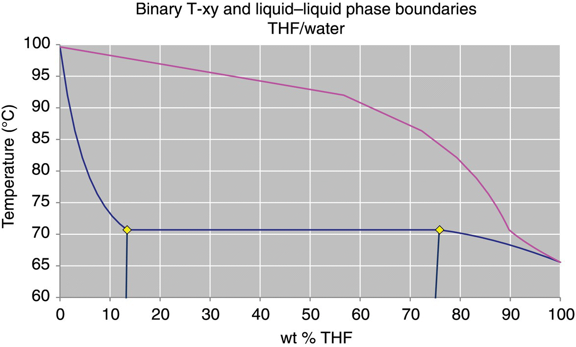
FIGURE 34.1 VLE of THF/water at 1000 mbar, UNIFAC model.
Source: From DynoChem VLLE utility.
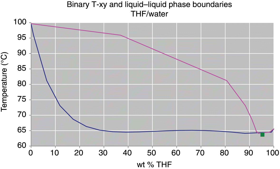
FIGURE 34.2 VLE of THF/water at 1000 mbar, NRTL model with square marker at location of azeotrope.
Source: From DynoChem VLLE utility.
34.3.2 In Silico Distillation Design
Advancements in in silico distillation modeling have made it possible to design and scale‐up a distillation process even in the absence of laboratory data. Over the last few decades, multiple software tools have aided in the process such as ASPEN, COSMOthermX, gPROMS, and DynoChem, among others. As outlined in Chapter 33, the following key parameters should be obtained for distillation design: (i) vapor pressure vs. temperature data and/or VLE data, (ii) solvent properties, and (iii) the heat transfer coefficient, UA, of the distillation vessel as a function of volume or details of vessel geometry. VLE data can be obtained, for example, via COSMOthermX or ASPEN as outlined in the Appendix 3.A, from DynoChem, or by internally developed tools. Most software provide a vapor–liquid and liquid–liquid equilibrium tool (VLLE tool) which contains the data for most commonly used solvents in the pharmaceutical industry. These tools are designed to generate thermodynamic phase diagrams for binary and ternary component systems. They calculate both VLE and liquid–liquid equilibrium (LLE) using standard activity coefficient methods to account for liquid‐phase nonideality. Most of these models treat the gas phase as an ideal gas as the components are common solvents at low pressure.
Most commonly available software implements UNIFAC [3], modified UNIFAC [5], UNIFAC LLE [6], or NRTL [4] for the liquid‐phase behavior. To model a distillation, two of the most popular VLE models are UNIFAC and NRTL. NRTL predictions are generally more accurate than those from UNIFAC and should be used when the required BIPs are available. In the case where NRTL BIPs are not available for solvents of interest, UNIFAC or its variant can be used; however, one should examine the predicted VLE T‐X,Y diagram carefully. Readers are encouraged to see Refs. [3–6] to understand the differences between NRTL, UNIFAC, and other UNIFAC variants.
If the solvent under consideration is not listed in the modeling tool, saturated vapor pressure of the solvent as a function of temperature needs to be determined from laboratory experiments. Alternatively, vapor pressure versus temperature data can be obtained from the DIPPR or DECHEMA database. Vapor pressure data is used to regress Antoine coefficients (A, B, and C; see Section 33.1.1.4), which are required to calculate NRTL BIPs. With the knowledge of Antoine coefficients and VLE data obtained from a database or experiments, NRTL BIPs can be fitted. Other relevant solvent properties such as density and heat capacity can be estimated from the DIPPR database as well. These solvent parameters can be taken back to the distillation model to design and optimize distillation processes.
In any VLLE tool used, special care should be taken to inquire for the presence of azeotropes. Azeotropes are not distillation boundaries for solvent swap distillation as fresh solvent is added to the solution. Continual solvent addition aids in pushing through the azeotrope boundary. However, when distillation is used to concentrate a solution and fresh solvent is not added, the distillation cannot move beyond the azeotrope composition, if one is present.
For distillation modeling, one other key piece of information required is the heat transfer coefficient (UA) of the distillation process vessel. Typically, models available can estimate UA of the distillation vessel if geometric details of the vessel, impeller details, solvents used, and service fluid are known. Overall, UA can be written as
where
- V is the instantaneous vessel volume.
UA should be estimated as a function of volume that can be used to make judicious decisions on holding volumes in constant volume or put‐and‐take distillations. To get a better estimate of UA, an engineering run can be performed using the plant distillation vessel with process‐relevant solvent. At any specified fill volume, the solution temperature and jacket temperature need to be recorded as a function of time; adequate mixing must be achieved in the reactor. The same experiment is repeated at different fill volumes. The experimental data should be fit to Eq. (34.1) to estimate UA as a function of volume.

FIGURE 34.3 VLE of isopropanol/THF at 180 mbar using the modified UNIFAC model.
Source: From DynoChem VLLE utility.
TABLE 34.2 Comparison of Distillation Time and Fresh Feed Required for Different Distillation Modes and Jacket Temperatures
| Scenario | Distillation Mode | Jacket Temperature (°C) | Vadd (L) | Total Distillation Time (h) | No. of Put‐and‐Takes | Volume of Fresh IPA Added (L) |
| 1. | CVD | 40 | — | 44 | — | 135 |
| 2. | Put‐and‐take | 40 | 50 | 48 | 4 | 177 |
| 3. | Put‐and‐take | 40 | 100 | 56 | 2 | 207 |
| 4. | CVD | 45 | — | 21 | — | 135 |
| 5. | Put‐and‐take | 45 | 50 | 23 | 4 | 205 |
| 6. | Put‐and‐take | 45 | 100 | 23 | 2 | 220 |
TABLE 34.3 Comparing the Impact of Concentrated Volume with Different Distillation Modes
| Scenario | Distillation Mode | Vconc (L) | Vadd (L) | Total Distillation Time (h) | No. of Put‐and‐Takes | Volume of Fresh IPA Added (L) |
| 1. | CVD | 150 | — | 24 | — | 273 |
| 2. | Put‐and‐take | 150 | 50 | 23 | 6 | 328 |
| 3. | Put‐and‐take | 150 | 100 | 24 | 4 | 391 |
| 4. | CVD | 300 | — | 25 | — | 542 |
| 5. | Put‐and‐take | 300 | 50 | 24 | 12 | 589 |
| 6. | Put‐and‐take | 300 | 100 | 25 | 6 | 620 |
34.4 CASE STUDIES ON THE USE OF DISTILLATION MODELS
34.4.1 Using Lab Data to Enhance a Distillation Model
A distillation was designed to reduce the concentration of water in a solution of THF and a dissolved substrate from 10 to less than 2 wt %. This reduction in water content can be achieved by concentrating the batch, followed by diluting with fresh solvent. The NRTL model was used to design and simulate the distillation, requiring 4 put‐and‐takes of 7 volumes at 200 mbar. Unfortunately, the simulations were predicting higher levels of water than what was observed in the lab. It was hypothesized that at high concentration (toward the end of the distillation) the dissolved substrate was influencing the VLE, perhaps due to an affinity for THF. Many times, nonvolatile, dissolved substrates are not included in a distillation model because their impact on the VLE of the solvent systems is negligible. This assumption does not always hold true, especially in processes where the batch is concentrated to a point where the substrate is a significant fraction of the mass. In these cases, the development of a VLE model that accurately predicts the system at hand is desirable.
In this case, a model that accurately predicts the solvent composition would enable in silico exploration of the operating space and greatly reduce the experimental burden to characterize this critical operation. In order to develop a model more representative of our specific system, a single batch distillation experiment was conducted at laboratory bench scale with a representative mixture of the substrate dissolved in wet THF (85 wt % THF, 15 wt % water on a solvent basis). The batch was heated to reflux and sampled, both batch and distillate, for solvent composition and the batch temperature recorded. The batch was concentrated intermittently to change the composition by directing distillate to a receiver and then sampling after re‐equilibration. This cycle was repeated until the batch composition reached 99 wt % THF on a solvent basis. It is important to collect batch and distillate stream samples at the same time, as these pairs of data points are needed to construct the T‐xy diagram. If automated sampling tools are available, this can enable sampling the two streams simultaneously. For distillations performed at atmospheric pressure, distillate samples can be taken directly from the condenser outlet. For distillations performed under reduced pressure, the distillate stream can be directed through a series of valves between the condenser and distillate receiver, allowing for isolation of a small amount of the distillate stream without breaking vacuum on the entire system. Distillate stream samples should not be taken directly from the distillate receiver, as they are not representative of the vapor phase at the given time point, but an accumulation of the distillate stream.
The plot in Figure 34.4 shows the data captured in this experiment. This data was then used to regress NRTL binary interaction parameters that could be used in further simulations of the distillation. These values are captured in Table 34.4 and compared with the values included in the DIPPR database.
FIGURE 34.4 VLE plot at 1000 mbar for THF/water with dissolved substrate present, from experimental data.
TABLE 34.4 Binary Interaction Parameters for THF/Water Solvent System
| NRTL Model BIPs | Δg12 (cal/mol) | Δg21 (cal/mol) | Alpha |
| From database | 915.7 | 1725 | 0.4522 |
| Regressed from experimental data | 916.0 | 1869 | 0.4472 |
The distillation was modeled using both the BIPs from the database and again with the experimentally fit BIPs. Using the database values, the model predicts that the batch will have 97.6 wt % water remaining under the previous outlined conditions, failing the specification. Using the experimentally fit BIPs, the model predicts the batch will have 98.7 wt % water remaining under the same process conditions, meeting the specification and aligning with experimental results. While that difference may not seem very significant, small amounts of water carried forward in a process can have significant impact on solubility or reactivity in downstream operations and may need to be carefully controlled. Refinement of the VLE model using experimental data enabled more accurate model predictions to be made and utilization of the model for in silico experimentation.
34.4.2 Selection of Solvent Pairs with Azeotropes to Improve Efficiency of Solvent Removal
A distillation process was being used to remove isobutanol and isopropanol from a solution of substrate dissolved in THF. Since residual isobutanol and isopropanol contributed to the formation of impurities in the subsequent reaction, each solvent needed to be reduced to very low levels (≤2 wt % total).
In this situation, the batch was concentrated by distillation to a minimum agitation volume, while the boiling point temperature was within the thermal stability range of the substrate. This was followed by addition of fresh THF and repeated until the desired isobutanol and isopropanol levels in the batch were obtained. In practice, 10 put‐and‐takes with THF were required to reach the desired levels.
From examination of the T‐xy diagram for THF and isobutanol at 50 mbar pressure (Figure 34.5), it becomes apparent that removing isobutanol from a solution of THF is inefficient. THF is much more volatile than isobutanol, so the vapor phase that is removed and condensed during a batch distillation is enriched in THF (as opposed to the preferred isobutanol). This mismatch in relative volatility of the desired solvent and undesired solvent is why 10 put‐and‐takes are necessary to arrive at the desired endpoint.

FIGURE 34.5 VLE for THF/isobutanol at 50 mabr.
Source: From DynoChem VLLE utility.
In order to optimize the process, the use of an alternate solvent that forms an azeotrope with isobutanol was explored. The existence of a minimum boiling point azeotrope between isobutanol and another solvent (n‐heptane in this case) facilitates the efficient removal of the less volatile component. When the batch composition lies on the right‐hand side of the azeotrope (see Figure 34.6), the vapor phase is enriched in isobutanol and results in greater removal of isobutanol compared to the THF/isobutanol system. This phenomenon can be observed between many organic solvents and water, allowing for efficient drying of organic solvent systems by batch distillation, even though the organic solvent is oftentimes the more volatile component. For the process discussed in this case study, the addition of n‐heptane reduced the required number of put‐and‐takes from ten to two and resulted in lower levels of isobutanol and isopropanol than the original process. It should be noted that n‐heptane was determined to be a suitable cosolvent to THF in the subsequent reaction, allowing for its use in this process.
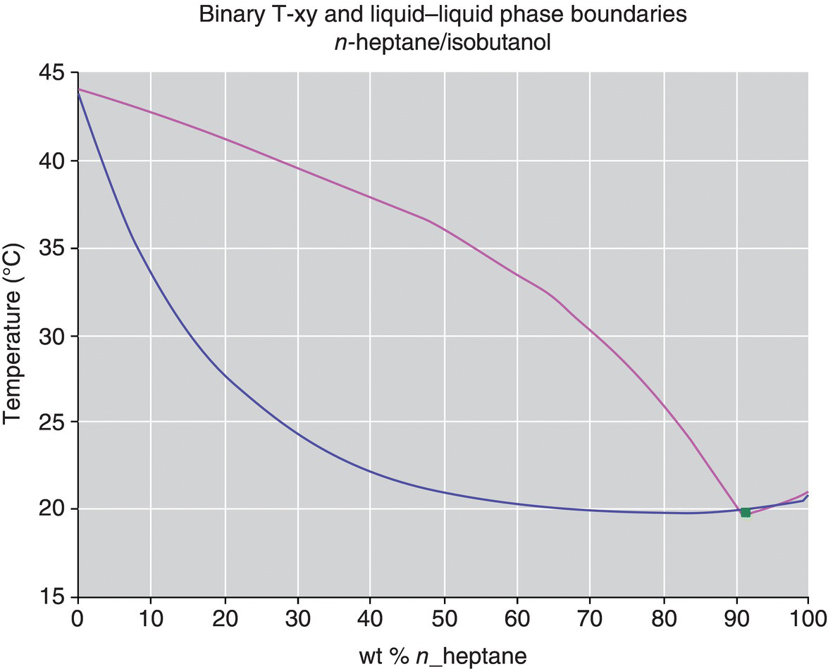
FIGURE 34.6 VLE for n‐heptane/isobutanol at 50 mabr.
Source: From DynoChem VLLE utility.
34.4.3 Optimization of Distillation Parameters to Enable Efficient Solvent Removal
In this case study, a solution of water‐saturated 2‐methyl tetrahydrofuran (2‐me THF) was being distilled to efficiently remove water from the system, which included a dissolved substrate. The presence of water combined with sufficiently high temperatures and long distillation times could lead to the formation of impurities. More broadly, undesired residual solvents present during isolation of an active pharmaceutical ingredient or intermediate can oftentimes, if present in sufficient quantities, lead to the formation of an undesired crystal form, impact particle size distribution following isolation, result in a difference in purification characteristics, or even form a new impurity. In this case study, distillation modeling was conducted to understand the impact of distillation parameters such as temperature and pressure on distillation time to achieve acceptable residual water content. Using this approach, the design space for the distillation was identified.
Figure 34.7 shows the results of distillation modeling performed using DynoChem. In this example, a range of pressures and temperatures were investigated and the resulting time to achieve the desired water content was calculated. Given a maximum distillation time of 30 hours, the distillation model helps define the optimal temperature and pressure and predicts the distillation time for a given temperature and pressure. In order to model the distillation time, it is necessary to calculate UA for the operating vessel (see Section 34.3.2 for more details). In this case study, a put‐and‐take distillation method was employed with a maximum solution temperature of 55 °C. The lowest obtainable pressure for the system under consideration was 100 mbar.

FIGURE 34.7 Distillation modeling to understand the temperature and pressure ranges that achieved a desired water limit in the user‐defined time frame.
Source: Model built in DynoChem.
It is well known that a lower operating pressure and a higher temperature during a batch distillation will result in a shorter distillation time when removing a trace solvent via a chase distillation. Distillation modeling in this case study, however, provided bounds for the pressure and temperature needed in a given manufacturing vessel, which would otherwise only be achievable by testing these parameters at scale. Using the predicted bounds, minimal experiments could be done to verify the boundaries of the design space where the process would be routinely operated. Equipment capabilities, such as the required temperature and pressure as well as the distillation mode, were also identified via the model.
34.4.4 Distillation as a Means of Crystallization (Evaporative Crystallization)
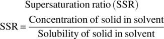
When tightly controlled crystallization is not a requirement for isolation, as is often the case with starting materials or early intermediates, crystallization via distillation can result in cycle time reduction. It is common to see both distillation and crystallization unit operations in the isolation process because the solvent used in the reaction may not be the desired solvent for the crystallization. To crystallize while distilling, also known as evaporative crystallization, solvent must be continuously removed until the solution is supersaturated. By carefully controlling the supersaturation ratio (Eq. 34.2) during distillation, crystallization kinetics can be controlled (to a limited extent), and particle growth can be achieved. It is important, however, to first understand the solubility of the solid mass throughout the solvent compositions encountered during the distillation so that the supersaturation ratio at any point in time can be calculated. The distillation rate can therefore be established, which results in the desired purity and physical properties attributes.
Evaporative crystallization can be modeled in DynoChem to provide additional insight into the crystallization process, optimize distillation parameters, and enable the design of a robust distillation and crystallization process. An example output from a DynoChem model for distillation as a means of crystallization is provided in Figure 34.8. The parameters chosen are those of a typical solid particle crystallizing from a mixture of 2‐me THF and water. The results shown are for a put‐and‐take simulation where water is being chase‐distilled with an excess of 2‐me THF. In this example, the solute was supersaturated at the beginning of the distillation process. Only a portion of the distillation is shown to provide an example of the output from an evaporative crystallization model. To model an evaporative crystallization process, solubility at numerous solvent compositions and temperatures should be obtained at the outset. The resulting solubility equation can be incorporated into the evaporative crystallization model. While multiple outputs can be used to assess the progression of the crystallization, two examples are shown in Figure 34.8. Monitoring the supersaturation ratio (SSR, calculated by applying Eq. (34.2) to the output data) with time in silico provides a means to understand the crystallization driving force. Modeling the fraction of solute crystallized provides a measurement of the expected yield. The SSR at any given time and the resulting fraction of solute that has been crystallized can be changed by varying the parameters discussed below.

FIGURE 34.8 Results from a DynoChem simulation of evaporative distillation of a model compound.
After creation of the initial model, it is possible to optimize the distillation process to influence the operating supersaturation ratio and consequently the crystallization rate. The model also calculates the total distillation time, which is impacted by a number of factors, most notably, the temperature, the pressure, the volume at which the distillation is performed, and the vessel's heat transfer properties. The impact of each of these parameters on the crystallization rate can be predicted through the evaporative crystallization DynoChem model.
Practical considerations when designing an evaporative crystallization process:
- Understand the product's solubility as a function of temperature and solvent composition to enable tighter control of the crystallization process.
- Carefully design the distillation/crystallization vessel, agitator, and agitation protocol considering the change in volume expected in the reactor during the course of the distillation. Understanding the impact of shear on particle attrition can aid in selecting the appropriate agitator design and agitation rate.
- The ability to make small changes to temperature and pressure in the distillation vessel enables control of the distillation through highly supersaturated regimes. Scale‐up from laboratory to the plant is nontrivial for evaporative distillation processes as the mechanisms of temperature and pressure control between the laboratory and plant, in particular, are distinctly different. Differences in heat transfer between laboratory and plant equipment [7] can present challenges in evaporative distillation scale‐up. In these scenarios, evaporative distillation models can be very useful to predict the temperature and pressure required to achieve the desired concentration as shown in this case study.
- Distillation modeling from the onset of process design followed by updating and verifying the model with experimental data aids in the utility of the model.
- Combining evaporative distillation with other traditional modes of crystallization, such as antisolvent, cooling, or reactive crystallization, can aid in maximizing yield [7]. Following crystallization, additional particle growth can be achieved via thermal ripening.
While there are several benefits to evaporative distillation, it is important to note that there may be challenges to this approach. The inherent inability to tightly control the distillation and therefore crystallization parameters could lead to uncontrolled crystallization. Controlling the nucleation rate is difficult due to the inhomogeneity of supersaturation as a result of temperature gradients throughout the vessel [7]. Due to this effect combined with volume reduction as a result of distillation, particles can form a crust on the reactor wall at the solid–liquid boundary as the volume of liquid in the crystallizer vessel is decreasing. This material is subject to high temperatures for an extended period of time and can result in unstable material that can decompose or result in impurity formation if the jacket temperature is not appropriately chosen [7]. Given the challenges that can be encountered to control the nucleation rate as well as particle encrustation in the reactor, attaining consistent physical properties from batch‐to‐batch can be difficult. If tight control of the product's physical properties is required, evaporative distillation may not be a good option. If the resulting isolated material following evaporative crystallization can meet the physical properties' requirements and leads to the desired yield and purity, combining distillation and crystallization can simplify the isolation process and reduce the isolation cycle time.
ACKNOWLEDGMENTS
We would like to thank Shailendra Bordawekar and Nandkishor Nere for the opportunity to author the chapter, Samrat Mukherjee and Moiz Diwan for critically reviewing sections of the chapter, Mathew Mulhern for discussions on distillation parameter selection, and the AbbVie API Pilot Plant for the exceptional execution and development of best practices for distillations.
Laurie Mlinar, Kushal Sinha, Elie Chaaya, and Subramanya Nayak are employees of AbbVie. The design, study conduct, and financial support for this research were provided by AbbVie. AbbVie participated in the interpretation of data, review, and approval of the publication.
REFERENCES
- 1. Wilson, G.M. (1964). Vapor‐liquid equilibrium. XI. A new expression for the excess free energy of mixing. Journal of the American Chemical Society 86 (2): 127–130.
- 2. Abrams, D.S. and Prausnitz, J.M. (1975). Statistical thermodynamics of liquid mixtures: a new expression for the excess Gibbs energy of partly or completely miscible systems. AIChE Journal 21 (1): 116–128.
- 3. Fredenslund, A., Jones, R.L., and Prausnitz, J.M. (1975). Group‐contribution estimation of activity coefficients in nonideal liquid mixtures. AIChE Journal 21: 1086.
- 4. Renon, H. and Prausnitz, J.M. (1968). Local compositions in thermodynamic excess functions for liquid mixtures. AIChE Journal 14 (1): 135–144.
- 5. Magnussen, T., Rasmussen, P., and Fredenslund, A. (1981). UNIFAC parameter table for prediction of liquid‐liquid equilibriums. Industrial and Engineering Chemistry Process Design and Development 20 (2): 331–339.
- 6. Gmehling, J., Li, J., and Schiller, M. (1993). A modified UNIFAC model. 2. Present parameter matrix and results for different thermodynamic properties. Industrial and Engineering Chemistry Research 32 (1): 178–193.
- 7. Tung, H.‐H., Paul, E.L., Midler, M., and McCauley, J.A. (2009). Evaporative crystallization. In: Crystallization of Organic Compounds: An Industrial Perspective. Hoboken, NJ: Wiley.