
1.4 Separable Equations and Applications
In the preceding sections we saw that if the function f(x, y) does not involve the variable y, then solving the first-order differential equation
is a matter of simply finding an antiderivative. For example, the general solution of
is given by
If instead f(x, y) does involve the dependent variable y, then we can no longer solve the equation merely by integrating both sides: The differential equation
differs from Eq. (2) only in the factor y appearing on the right-hand side, but this is enough to prevent us from using the same approach to solve Eq. (3a) that was successful with Eq. (2).
And yet, as we will see throughout the remainder of this chapter, differential equations like (3a) often can, in fact, be solved by methods which are based on the idea of “integrating both sides.” The idea behind these techniques is to rewrite the given equation in a form that, while equivalent to the given equation, allows both sides to be integrated directly, thus leading to the solution of the original differential equation.
The most basic of these methods, separation of variables, can be applied to Eq. (3a). First, we note that the right-hand function f(x,y)=−6xy
Next, we informally break up the derivative dy/dx
Equation (3c) is an equivalent version of the original differential equation in (3a), but with the variables x and y separated (that is, by the equal sign), and this is what allows us to integrate both sides. The left-hand side is integrated with respect to y (with no “interference” from the variable x), and vice versa for the right-hand side. This leads to
or
This gives the general solution of Eq. (3a) implicitly, and a family of solution curves is shown in Fig. 1.4.1.
In this particular case we can go on to solve for y to give the explicit general solution

FIGURE 1.4.1.
Slope field and solution curves for y′=−6xy
where A represents the constant ±eC
which is the upper emphasized solution curve shown in Fig. 1.4.1. In the same way, the initial condition y(0)=−4
which is the lower emphasized solution curve shown in Fig. 1.4.1.
To complete this example, we note that whereas the constant A in Eq. (5) is nonzero, taking A=0
In general, the first-order differential equation (1) is called separable provided that f(x,y)
where h(y)=1/k(y)
which we understand to be concise notation for the differential equation
(In the preceding example, h(y)=1y
equivalently,
All that is required is that the antiderivatives
can be found. To see that Eqs. (6) and (7) are equivalent, note the following consequence of the chain rule:
which in turn is equivalent to
because two functions have the same derivative on an interval if and only if they differ by a constant on that interval.
Example 1
Solve the differential equation
Solution
Because
is the product of a function that depends only on x, and one that depends only on y, Eq. (9) is separable, and thus we can proceed in much the same way as in Eq. (3a). Before doing so, however, we note an important feature of Eq. (9) not shared by Eq. (3a): The function k(y)=13y2−5
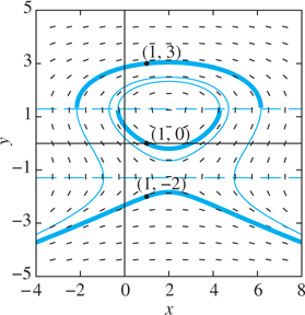
FIGURE 1.4.2.
Slope field and solution curves for y′=(4−2x)/(3y2−5)
What this means for the differential equation (9) is that no solution curve of this equation can cross either of the horizontal lines y=±√53
With this in mind, the general solution of the differential equation in Eq. (9) is easy to find, at least in implicit form. Separating variables and integrating both sides leads to
and thus
Note that unlike Eq. (4), the general solution in Eq. (10) cannot readily be solved for y; thus we cannot directly plot the solution curves of Eq. (9) in the form y=y(x)
This shows that the solution curves of the differential equation in Eq. (9) are contained in the level curves (also known as contours) of the function
Because no particular solution curve of Eq. (9) can cross either of the lines y=±√53
For example, suppose that we wish to solve the initial value problem
Substituting x=1
of F(x, y); Fig. 1.4.2 shows this and other level curves of F(x, y). However, because the solution curve of the initial value problem (13) must pass through the point (1, 3), which lies above the line y=√53
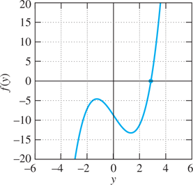
FIGURE 1.4.3.
Graph of f(y)=y3−5y−9
Finally, despite the difficulty of solving Eq. (14) for y by algebraic means, we can nonetheless “solve” for y in the sense that, when a specific value of x is substituted in (14), we can attempt to solve numerically for y. For instance, taking x=4
Fig. 1.4.3 shows the graph of f. Using technology we can solve for the single real root y≈2.8552
| x | −1 |
0 | 1 | 2 | 3 | 4 | 5 | 6 |
| y | 2.5616 | 2.8552 | 3 | 3.0446 | 3 | 2.8552 | 2.5616 | 1.8342 |
Implicit, General, and Singular Solutions
The equation K(x,y)=0
so x2+y2=4
satisfies the initial condition y(0)=2
Remark 1
You should not assume that every possible algebraic solution y=y(x)
that yields (or “contains”) not only the previously noted explicit solutions y=+√4−x2

FIGURE 1.4.4.
Slope field and solution curves for y′=−x/y
Remark 2
Similarly, solutions of a given differential equation can be either gained or lost when it is multiplied or divided by an algebraic factor. For instance, consider the differential equation
having the obvious solution y=2x
of which y=2x
A solution of a differential equation that contains an “arbitrary constant” (like the constant C appearing in Eqs. (4) and (10)) is commonly called a general solution of the differential equation; any particular choice of a specific value for C yields a single particular solution of the equation.
The argument preceding Example 1 actually suffices to show that every particular solution of the differential equation h(y)y′=g(x)

FIGURE 1.4.5.
The general solution curves y=(x−C)2
In Section 1.5 we shall see that every particular solution of a linear first-order differential equation is contained in its general solution. By contrast, it is common for a nonlinear first-order differential equation to have both a general solution involving an arbitrary constant C and one or several particular solutions that cannot be obtained by selecting a value for C. These exceptional solutions are frequently called singular solutions. In Problem 30 we ask you to show that the general solution of the differential equation (y′)2=4y
Example 2
Find all solutions of the differential equation
Solution
Separation of variables gives
Positive values of the arbitrary constant C give the solution curves in Fig. 1.4.6 that lie above the line y=1

FIGURE 1.4.6.
General and singular solution curves for y′=6x(y−1)2/3
Natural Growth and Decay
The differential equation
![]()
serves as a mathematical model for a remarkably wide range of natural phenomena—any involving a quantity whose time rate of change is proportional to its current size. Here are some examples.
Population Growth: Suppose that P(t) is the number of individuals in a population (of humans, or insects, or bacteria) having constant birth and death rates β
and therefore
where k=β−δ
Compound Interest: Let A(t) be the number of dollars in a savings account at time t (in years), and suppose that the interest is compounded continuously at an annual interest rate r. (Note that 10% annual interest means that r=0.10
Radioactive Decay: Consider a sample of material that contains N(t) atoms of a certain radioactive isotope at time t. It has been observed that a constant fraction of those radioactive atoms will spontaneously decay (into atoms of another element or into another isotope of the same element) during each unit of time. Consequently, the sample behaves exactly like a population with a constant death rate and no births. To write a model for N(t), we use Eq. (18) with N in place of P, with k>0
The value of k depends on the particular radioactive isotope.
The key to the method of radiocarbon dating is that a constant proportion of the carbon atoms in any living creature is made up of the radioactive isotope C14
The ratio of C14
Of course, when a living organism dies, it ceases its metabolism of carbon and the process of radioactive decay begins to deplete its C14
(Matters are not as simple as we have made them appear. In applying the technique of radiocarbon dating, extreme care must be taken to avoid contaminating the sample with organic matter or even with ordinary fresh air. In addition, the cosmic ray levels apparently have not been constant, so the ratio of C14
Drug Elimination: In many cases the amount A(t) of a certain drug in the bloodstream, measured by the excess over the natural level of the drug, will decline at a rate proportional to the current excess amount. That is,
where λ>0
The Natural Growth Equation
The prototype differential equation dx/dt=kx
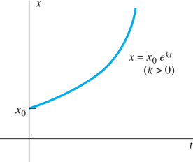
FIGURE 1.4.7.
Natural growth.
Then we solve for x:
Because C is a constant, so is A=eC
![]()
Because of the presence of the natural exponential function in its solution, the differential equation
![]()
is often called the exponential or natural growth equation. Figure 1.4.7 shows a typical graph of x(t) in the case k>0

FIGURE 1.4.8.
Natural decay.
Example 3
World population According to data listed at www.census.gov, the world’s total population reached 6 billion persons in mid-1999, and was then increasing at the rate of about 212 thousand persons each day. Assuming that natural population growth at this rate continues, we want to answer these questions:
What is the annual growth rate k?
What will be the world population at the middle of the 21st century?
How long will it take the world population to increase tenfold—thereby reaching the 60 billion that some demographers believe to be the maximum for which the planet can provide adequate food supplies?
Solution
We measure the world population P(t) in billions and measure time in years. We take t=0
t=0 to correspond to (mid) 1999, so P0=6P0=6 . The fact that P is increasing by 212,000, or 0.000212 billion, persons per day at time t=0t=0 means thatP′(0)=(0.000212)(365.25)≈0.07743P'(0)=(0.000212)(365.25)≈0.07743 billion per year. From the natural growth equation P′=kP
P'=kP with t=0t=0 we now obtaink=P′(0)P(0)≈0.077436≈0.0129.k=P'(0)P(0)≈0.077436≈0.0129. Thus the world population was growing at the rate of about 1.29% annually in 1999. This value of k gives the world population function
P(t)=6e0.0129t.P(t)=6e0.0129t. With t=51
t=51 we obtain the predictionP(51)=6e(0.0129)(51)≈11.58 (billion)P(51)=6e(0.0129)(51)≈11.58 (billion) for the world population in mid-2050 (so the population will almost have doubled in the just over a half-century since 1999).
The world population should reach 60 billion when
60=6e0.0129t;that is, when t = ln 100.0129≈ 178;60=6e0.0129t;that is, when t = ln 100.0129≈ 178; and thus in the year 2177.
Note
Actually, the rate of growth of the world population is expected to slow somewhat during the next half-century, and the best current prediction for the 2050 population is “only” 9.1 billion. A simple mathematical model cannot be expected to mirror precisely the complexity of the real world.
The decay constant of a radioactive isotope is often specified in terms of another empirical constant, the half-life of the isotope, because this parameter is more convenient. The half-life τ
For example, the half-life of C14
Example 4
Radiometric dating A specimen of charcoal found at Stonehenge turns out to contain 63% as much C14
Solution
We take t=0
Thus the sample is about 3800 years old. If it has any connection with the builders of Stonehenge, our computations suggest that this observatory, monument, or temple—whichever it may be—dates from 1800 b.c. or earlier.
Cooling and Heating
According to Newton’s law of cooling (Eq. (3) of Section 1.1), the time rate of change of the temperature T(t) of a body immersed in a medium of constant temperature A is proportional to the difference A−T
where k is a positive constant. This is an instance of the linear first-order differential equation with constant coefficients:
![]()
It includes the exponential equation as a special case (b=0
Example 5
Cooling A 4-lb roast, initially at 50°F
Solution
We take time t in minutes, with t=0
Now T(0)=50
Hence we finally solve the equation
for t=−[ln (225/325)]/(0.0035)≈105
Torricelli’s Law
Suppose that a water tank has a hole with area a at its bottom, from which water is leaking. Denote by y(t) the depth of water in the tank at time t, and by V(t) the volume of water in the tank then. It is plausible—and true, under ideal conditions—that the velocity of water exiting through the hole is
which is the velocity a drop of water would acquire in falling freely from the surface of the water to the hole (see Problem 35 of Section 1.2). One can derive this formula beginning with the assumption that the sum of the kinetic and potential energy of the system remains constant. Under real conditions, taking into account the constriction of a water jet from an orifice, v=c√2gy
As a consequence of Eq. (27), we have
![]()
equivalently,
![]()
This is a statement of Torricelli’s law for a draining tank. Let A(y) denote the horizontal cross-sectional area of the tank at height y. Then, applied to a thin horizontal slice of water at height ̲y with area A(̲y) and thickness d̲y, the integral calculus method of cross sections gives
The fundamental theorem of calculus therefore implies that dV/dy=A(y) and hence that
From Eqs. (28) and (29) we finally obtain
an alternative form of Torricelli’s law.
Example 6
Draining tank A hemispherical bowl has top radius 4 ft and at time t=0 is full of water. At that moment a circular hole with diameter 1 in. is opened in the bottom of the tank. How long will it take for all the water to drain from the tank?
Solution
From the right triangle in Fig. 1.4.9, we see that
With g=32 ft/s2, Eq. (30) becomes
Now y(0)=4, so
The tank is empty when y=0, thus when
that is, about 35 min 50 s. So it takes slightly less than 36 min for the tank to drain.

FIGURE 1.4.9.
Draining a hemispherical tank.
Example 7
In the case of an upright cylindrical tank with constant cross-sectional area A, Torricelli’s law in Eq. (30) takes the form
with c=k/A. With initial condition y(0)=0 we routinely separate variables and integrate to get
However, this formula if taken at face value implies that y>0 if t>0. But if the tank is empty at time t=0 as prescribed by the initial condition y(0)=0, then certainly the tank remains empty thereafter, so y(t)≡0 for t>0.
To see what is going on here, note that the right-hand side function f(t,y)=−c√y in our differential equation y′=−c√y does not satisfy the condition that ∂f/∂y be continuous at (0, 0), so the existence-uniqueness theorem of Section 1.3 does not guarantee uniqueness of a solution near t=0. Indeed, we note the two different but physically meaningful solutions
of the initial value problem y′=−c√y, y(0)=0. The constant solution y1(t)≡0 corresponds to a tank that always has been and always will be empty, while y2(t) corresponds to a tank draining while t<0 that empties precisely at time t=0 and remains empty thereafter.
Thus this example provides a concrete physical situation described by an initial value problem with non-unique solutions.
1.4 Problems
Find general solutions (implicit if necessary, explicit if convenient) of the differential equations in Problems 1 through 18. Primes denote derivatives with respect to x.
dydx+2xy=0
dydx+2xy2=0
dydx=ysin x
(1+x)dydx=4y
2√xdydx=√1−y2
dydx=3√xy
dydx=(64xy)1/3
dydx=2xsecy
(1−x2)dydx=2y
(1+x)2dydx=(1+y)2
y′=xy3
yy′=x(y2+1)
y3dydx=(y4+1) cos x
dydx=1+√x1+√y
dydx=(x−1)y5x2(2y3−y)
(x2+1)(tany)y′=x
y′=1+x+y+xy (Suggestion: Factor the right-hand side.)
x2y′=1−x2+y2−x2y2
Find explicit particular solutions of the initial value problems in Problems 19 through 28.
dydx=yex, y(0)=2e
dydx=3x2(y2+1), y(0)=1
2ydydx=x√x2−16, y(5)=2
dydx=4x3y−y, y(1)=−3
dydx+1=2y, y(1)=1
dydx=ycotx, y(12π)=12π
xdydx−y=2x2y, y(1)=1
dydx=2xy2+3x2y2, y(1)=−1
dydx=6e2x−y,y(0)=0
2√xdydx=cos2 y,y(4)=π/4
Problems 29 through 32 explore the connections among general and singular solutions, existence, and uniqueness.
(a) Find a general solution of the differential equation dy/dx=y2. (b) Find a singular solution that is not included in the general solution. (c) Inspect a sketch of typical solution curves to determine the points (a, b) for which the initial value problem y′=y2, y(a)=b has a unique solution.
Solve the differential equation (dy/dx)2=4y to verify the general solution curves and singular solution curve that are illustrated in Fig. 1.4.5. Then determine the points (a, b) in the plane for which the initial value problem (y′)2=4y, y(a)=b has (a) no solution, (b) infinitely many solutions that are defined for all x, (c) on some neighborhood of the point x=a, only finitely many solutions.
Discuss the difference between the differential equations (dy/dx)2=4y and dy/dx=2√y. Do they have the same solution curves? Why or why not? Determine the points (a, b) in the plane for which the initial value problem y′=2√y, y(a)=b has (a) no solution, (b) a unique solution, (c) infinitely many solutions.
Find a general solution and any singular solutions of the differential equation dy/dx=y√y2−1. Determine the points (a, b) in the plane for which the initial value problem y′=y√y2−1, y(a)=b has (a) no solution, (b) a unique solution, (c) infinitely many solutions.
Population growth A certain city had a population of 25,000 in 1960 and a population of 30,000 in 1970. Assume that its population will continue to grow exponentially at a constant rate. What population can its city planners expect in the year 2000?
Population growth In a certain culture of bacteria, the number of bacteria increased sixfold in 10 h. How long did it take for the population to double?
Radiocarbon dating Carbon extracted from an ancient skull contained only one-sixth as much C14 as carbon extracted from present-day bone. How old is the skull?
Radiocarbon dating Carbon taken from a purported relic of the time of Christ contained 4.6×10¹⁰ atoms of C14 per gram. Carbon extracted from a present-day specimen of the same substance contained 5.0×10¹⁰ atoms of C14 per gram. Compute the approximate age of the relic. What is your opinion as to its authenticity?
Continuously compounded interest Upon the birth of their first child, a couple deposited $5000 in an account that pays 8% interest compounded continuously. The interest payments are allowed to accumulate. How much will the account contain on the child’s eighteenth birthday?
Continuously compounded interest Suppose that you discover in your attic an overdue library book on which your grandfather owed a fine of 30 cents 100 years ago. If an overdue fine grows exponentially at a 5% annual rate compounded continuously, how much would you have to pay if you returned the book today?
Drug elimination Suppose that sodium pentobarbital is used to anesthetize a dog. The dog is anesthetized when its bloodstream contains at least 45 milligrams (mg) of sodium pentobarbitol per kilogram of the dog’s body weight. Suppose also that sodium pentobarbitol is eliminated exponentially from the dog’s bloodstream, with a half-life of 5 h. What single dose should be administered in order to anesthetize a 50-kg dog for 1 h?
Radiometric dating The half-life of radioactive cobalt is 5.27 years. Suppose that a nuclear accident has left the level of cobalt radiation in a certain region at 100 times the level acceptable for human habitation. How long will it be until the region is again habitable? (Ignore the probable presence of other radioactive isotopes.)
Isotope formation Suppose that a mineral body formed in an ancient cataclysm—perhaps the formation of the earth itself—originally contained the uranium isotope U238 (which has a half-life of 4.51×10⁹ years) but no lead, the end product of the radioactive decay of U238. If today the ratio of U238 atoms to lead atoms in the mineral body is 0.9, when did the cataclysm occur?
Radiometric dating A certain moon rock was found to contain equal numbers of potassium and argon atoms. Assume that all the argon is the result of radioactive decay of potassium (its half-life is about 1.28×10⁹ years) and that one of every nine potassium atom disintegrations yields an argon atom. What is the age of the rock, measured from the time it contained only potassium?
Cooling A pitcher of buttermilk initially at 25°C is to be cooled by setting it on the front porch, where the temperature is 0°C. Suppose that the temperature of the buttermilk has dropped to 15°C after 20 min. When will it be at 5°C?
Solution rate When sugar is dissolved in water, the amount A that remains undissolved after t minutes satisfies the differential equation dA/dt=−kA (k>0). If 25% of the sugar dissolves after 1 min, how long does it take for half of the sugar to dissolve?
Underwater light intensity The intensity I of light at a depth of x meters below the surface of a lake satisfies the differential equation dI/dx=(−1.4)I. (a) At what depth is the intensity half the intensity I0 at the surface (where x=0)? (b) What is the intensity at a depth of 10 m (as a fraction of I0)? (c) At what depth will the intensity be 1% of that at the surface?
Barometric pressure and altitude The barometric pressure p (in inches of mercury) at an altitude x miles above sea level satisfies the initial value problem dp/dx=(−0.2)p, p(0)=29.92. (a) Calculate the barometric pressure at 10,000 ft and again at 30,000 ft. (b) Without prior conditioning, few people can survive when the pressure drops to less than 15 in. of mercury. How high is that?
Spread of rumor A certain piece of dubious information about phenylethylamine in the drinking water began to spread one day in a city with a population of 100,000. Within a week, 10,000 people had heard this rumor. Assume that the rate of increase of the number who have heard the rumor is proportional to the number who have not yet heard it. How long will it be until half the population of the city has heard the rumor?
Isotope formation According to one cosmological theory, when uranium was first generated in the early evolution of the universe following the “big bang,” the isotopes U235 and U238 were produced in equal amounts. Given the half-lives of 4.51×10⁹ years for U238 and 7.10×10⁸ years for U235, calculate the length of time required to reach the present distribution of 137.7 atoms of U238 for each atom of U235.
Cooling A cake is removed from an oven at 210°F and left to cool at room temperature, which is 70°F. After 30 min the temperature of the cake is 140°F. When will it be 100°F?
Pollution increase The amount A(t) of atmospheric pollutants in a certain mountain valley grows naturally and is tripling every 7.5 years.
If the initial amount is 10 pu (pollutant units), write a formula for A(t) giving the amount (in pu) present after t years.
What will be the amount (in pu) of pollutants present in the valley atmosphere after 5 years?
If it will be dangerous to stay in the valley when the amount of pollutants reaches 100 pu, how long will this take?
Radioactive decay An accident at a nuclear power plant has left the surrounding area polluted with radioactive material that decays naturally. The initial amount of radioactive material present is 15 su (safe units), and 5 months later it is still 10 su.
Write a formula giving the amount A(t) of radioactive material (in su) remaining after t months.
What amount of radioactive material will remain after 8 months?
How long—total number of months or fraction thereof—will it be until A=1 su, so it is safe for people to return to the area?
Growth of languages There are now about 3300 different human “language families” in the whole world. Assume that all these are derived from a single original language and that a language family develops into 1.5 language families every 6 thousand years. About how long ago was the single original human language spoken?
Growth of languages Thousands of years ago ancestors of the Native Americans crossed the Bering Strait from Asia and entered the western hemisphere. Since then, they have fanned out across North and South America. The single language that the original Native Americans spoke has since split into many Indian “language families.” Assume (as in Problem 52) that the number of these language families has been multiplied by 1.5 every 6000 years. There are now 150 Native American language families in the western hemisphere. About when did the ancestors of today’s Native Americans arrive?
Torricelli’s Law
Problems 54 through 64 illustrate the application of Torricelli’s law.
A tank is shaped like a vertical cylinder; it initially contains water to a depth of 9 ft, and a bottom plug is removed at time t=0 (hours). After 1 h the depth of the water has dropped to 4 ft. How long does it take for all the water to drain from the tank?
Suppose that the tank of Problem 54 has a radius of 3 ft and that its bottom hole is circular with radius 1 in. How long will it take the water (initially 9 ft deep) to drain completely?
At time t=0 the bottom plug (at the vertex) of a full conical water tank 16 ft high is removed. After 1 h the water in the tank is 9 ft deep. When will the tank be empty?
Suppose that a cylindrical tank initially containing V0 gallons of water drains (through a bottom hole) in T minutes. Use Torricelli’s law to show that the volume of water in the tank after t≦T minutes is V=V0[1−(t/T)]2.
A water tank has the shape obtained by revolving the curve y=x4/3 around the y-axis. A plug at the bottom is removed at 12 noon, when the depth of water in the tank is 12 ft. At 1 p.m. the depth of the water is 6 ft. When will the tank be empty?
A water tank has the shape obtained by revolving the parabola x2=by around the y-axis. The water depth is 4 ft at 12 noon, when a circular plug in the bottom of the tank is removed. At 1 p.m. the depth of the water is 1 ft.(a) Find the depth y(t) of water remaining after t hours.(b) When will the tank be empty?(c) If the initial radius of the top surface of the water is 2 ft, what is the radius of the circular hole in the bottom?
A cylindrical tank with length 5 ft and radius 3 ft is situated with its axis horizontal. If a circular bottom hole with a radius of 1 in. is opened and the tank is initially half full of water, how long will it take for the liquid to drain completely?
A spherical tank of radius 4 ft is full of water when a circular bottom hole with radius 1 in. is opened. How long will be required for all the water to drain from the tank?
Suppose that an initially full hemispherical water tank of radius 1 m has its flat side as its bottom. It has a bottom hole of radius 1 cm. If this bottom hole is opened at 1 p.m., when will the tank be empty?
Consider the initially full hemispherical water tank of Example 8, except that the radius r of its circular bottom hole is now unknown. At 1 p.m. the bottom hole is opened and at 1:30 p.m. the depth of water in the tank is 2 ft.(a) Use Torricelli’s law in the form dV/dt=−(0.6)πr2√2gy (taking constriction into account) to determine when the tank will be empty. (b) What is the radius of the bottom hole?
A 12 h water clock is to be designed with the dimensions shown in Fig. 1.4.10, shaped like the surface obtained by revolving the curve y=f(x) around the y-axis. What should this curve be, and what should the radius of the circular bottom hole be, in order that the water level will fall at the constant rate of 4 inches per hour (in./h)?
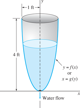
FIGURE 1.4.10.
The clepsydra.
Time of death Just before midday the body of an apparent homicide victim is found in a room that is kept at a constant temperature of 70°F. At 12 noon the temperature of the body is 80°F and at 1 p.m. it is 75°F. Assume that the temperature of the body at the time of death was 98.6°F and that it has cooled in accord with Newton’s law. What was the time of death?
Snowplow problem Early one morning it began to snow at a constant rate. At 7 a.m. a snowplow set off to clear a road. By 8 a.m. it had traveled 2 miles, but it took two more hours (until 10 a.m.) for the snowplow to go an additional 2 miles.(a) Let t=0 when it began to snow, and let x denote the distance traveled by the snowplow at time t. Assuming that the snowplow clears snow from the road at a constant rate (in cubic feet per hour, say), show that
kdxdt=1twhere k is a constant. (b) What time did it start snowing? (Answer: 6 a.m.)
Snowplow problem A snowplow sets off at 7 a.m. as in Problem 66. Suppose now that by 8 a.m. it had traveled 4 miles and that by 9 a.m. it had moved an additional 3 miles. What time did it start snowing? This is a more difficult snowplow problem because now a transcendental equation must be solved numerically to find the value of k. (Answer: 4:27 a.m.)
Brachistochrone Figure 1.4.11 shows a bead sliding down a frictionless wire from point P to point Q. The brachistochrone problem asks what shape the wire should be in order to minimize the bead’s time of descent from P to Q. In June of 1696, John Bernoulli proposed this problem as a public challenge, with a 6-month deadline (later extended to Easter 1697 at George Leibniz’s request). Isaac Newton, then retired from academic life and serving as Warden of the Mint in London, received Bernoulli’s challenge on January 29, 1697. The very next day he communicated his own solution—the curve of minimal descent time is an arc of an inverted cycloid—to the Royal Society of London. For a modern derivation of this result, suppose the bead starts from rest at the origin P and let y=y(x) be the equation of the desired curve in a coordinate system with the y-axis pointing downward. Then a mechanical analogue of Snell’s law in optics implies that
sinαv= constant,(i)where α denotes the angle of deflection (from the vertical) of the tangent line to the curve—so cotα=y′(x) (why?)—and v=√2gy is the bead’s velocity when it has descended a distance y vertically (from KE=12mv2=mgy=−PE).

FIGURE 1.4.11.
A bead sliding down a wire—the brachistochrone problem.
First derive from Eq. (i) the differential equation
dydx=√2a−yy,(ii)where a is an appropriate positive constant.
Substitute y=2asin2 t, dy=4asin tcos t dt in (ii) to derive the solution
x=a(2t−sin 2t), y=a(1−cos 2t)(iii)for which t=y=0 when x=0. Finally, the substitution of θ=2t in (iii) yields the standard parametric equations x=a(θ−sin θ), y=a(1−cos θ) of the cycloid that is generated by a point on the rim of a circular wheel of radius a as it rolls along the x-axis. [See Example 5 in Section 9.4 of Edwards and Penney, Calculus: Early Transcendentals, 7th edition, Hoboken, NJ: Pearson, 2008.]
Hanging cable Suppose a uniform flexible cable is suspended between two points (±L,H) at equal heights located symmetrically on either side of the x-axis (Fig. 1.4.12). Principles of physics can be used to show that the shape y=y(x) of the hanging cable satisfies the differential equation
ad2ydx2=√1+(dydx)2,where the constant a=T/ρ is the ratio of the cable’s tension T at its lowest point x=0 (where y′(0)=0) and its (constant) linear density ρ. If we substitute v=dy/dx, dv/dx=d2y/dx2 in this second-order differential equation, we get the first-order equation
advdx=√1+v2.Solve this differential equation for y′(x)=v(x)=sinh(x/a). Then integrate to get the shape function
y(x)= a cosh(xa) +Cof the hanging cable. This curve is called a catenary, from the Latin word for chain.

FIGURE 1.4.12.
The catenary.
1.4 Application The Logistic Equation
As in Eq. (7) of this section, the solution of a separable differential equation reduces to the evaluation of two indefinite integrals. It is tempting to use a symbolic algebra system for this purpose. We illustrate this approach using the logistic differential equation
that models a population x(t) with births (per unit time) proportional to x and deaths proportional to x2. Here we concentrate on the solution of Eq. (1) and defer discussion of population applications to Section 2.1.
If a=0.01 and b=0.0001, for instance, Eq. (1) is
Separation of variables leads to
We can evaluate the integral on the left by using the Maple command
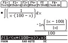
FIGURE 1.4.13.
TI-89 screen showing the integral in Eq. (3).
int(1/(x∗(100 - x)), x);the Mathematica command
Integrate[ 1/(x∗(100 - x)), x ]or the Matlab command
syms x; int(1/(x∗(100 - x) ) )Alternatively, we could use the freely available Wolfram|Alpha system (www.wolframalpha.com); the query
integrate 1/(x*(100 - x) )produces the output shown in Fig. 1.4.14.

FIGURE 1.4.14.
Wolfram|Alpha display showing the integral in Eq. (3). Screenshot of Wolfram|Alpha output. Used by permission of WolframAlpha LLC.
Any computer algebra system gives a result of the form
equivalent to the graphing calculator result shown in Fig. 1.4.13.
You can now apply the initial condition x(0)=x0, combine logarithms, and finally exponentiate to solve Eq. (4) for the particular solution
of Eq. (2). The slope field and solution curves shown in Fig. 1.4.15 suggest that, whatever is the initial value x0, the solution x(t) approaches 100 as t→+∞. Can you use Eq. (5) to verify this conjecture?
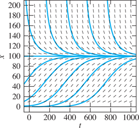
FIGURE 1.4.15.
Slope field and solution curves for x′=(0.01)x−(0.0001)x2.
Investigation: For your own personal logistic equation, take a=m/n and b=1/n in Eq. (1), with m and n being the largest two distinct digits (in either order) in your student ID number.
First generate a slope field for your differential equation and include a sufficient number of solution curves that you can see what happens to the population as t→+∞. State your inference plainly.
Next use a computer algebra system to solve the differential equation symbolically; then use the symbolic solution to find the limit of x(t) as t→+∞. Was your graphically based inference correct?
Finally, state and solve a numerical problem using the symbolic solution. For instance, how long does it take x to grow from a selected initial value x0 to a given target value x1?