
3
PROCESS SAFETY AND REACTION HAZARD ASSESSMENT
Wim Dermaut
Chemical Process Development, Materials Technology Center, Agfa‐Gevaert NV, Mortsel, Belgium
3.1 INTRODUCTION
When the issue of safety is raised in the context of pharmaceutical manufacturing, many might first think about issues of product and/or patient safety. There is another side of safety that might not get as much attention but that is also crucial to the production of pharmaceuticals: process safety. An often heard phrase in this context is “If the process can't be run safely, it shouldn't be run at all.” Process safety should indeed be a concern, starting already in early development of a drug candidate. Running a small‐scale synthesis in the lab only once is one thing, and running this process at metric ton scale on a routine basis in a chemical manufacturing plant is something completely different. Events such as exothermicity, gas generation, and stability of products might be relatively unimportant on a small scale, but they can pose tremendous challenges when this reaction is run at a larger scale.
This chapter provides an introduction to the field of process safety. The aim is to discuss some of the fundamentals of safety testing, in order to try to facilitate the communication between chemical engineers and development chemists. The focus will be on the interpretation and practical use of the different test results rather than on the tests itself. The discussion will focus mainly on (semi‐) batch reactors, since this is still the most commonly used type of reactors. Some brief thoughts on the impact of flow chemistry on process safety will be added as well.
This chapter can be roughly divided in four main parts. We will start with a brief description of some general concepts like the runaway scenario and the criticality classes. After that, we will consider some safety aspects of the desired synthesis reaction and how it can be studied on the lab scale. The main focus will be on exothermicity (heat generation) and gas generation. We will then continue discussing how the data thus obtained can be used to scale‐up the reaction safely, with a large emphasis on the heat transfer at a large scale. Finally we will take a closer look at the undesired decomposition reactions that can take place in the case of process deviations, how to study them at lab scale and how to minimize the associated risks.
In the next paragraphs, the reader is offered some first insights into the domain of process safety and safety testing. It is by no means the intention of the author to give an exhaustive overview of this field, but hopefully this introduction can provide some insight into the most common pitfalls of process safety. For a more in‐depth review, the reader is referred to the widely available literature [1–3].
3.2 GENERAL CONCEPTS
3.2.1 Runaway Scenario
When discussing process safety, the cooling failure scenario is often used to illustrate the possibility of a runaway reaction in a reactor [4, 5]. In Figure 3.1, a possible cooling failure scenario is depicted. The normal process condition is indicated with the thin solid line: the reactants are being charged to the reactor (batch reaction), the reaction mixture is heated to the desired process temperature (Tp), the mixture is then kept isothermally at this temperature with active jacket cooling (exothermic reaction), and when the reaction is finished, the mixture is brought back to room temperature for further workup. This is the process as it is intended to be run both at small scale in the lab and at larger scale in the plant.

FIGURE 3.1 Cooling failure scenario. The thin line represents the normal mode of operation, the thick line represents the possible consequences of a cooling failure [3].
Source: Reproduced with permission from Stoessel [3]. Copyright 2008 Wiley‐VCH Verlag GmbH & Co. KGaA.
Let us now consider the possible consequences of a loss of cooling. We will assume that the loss of cooling power occurs relatively short after the desired process temperature has been reached, as indicated in the graph. From this point on, the exothermic reaction will proceed, but since the reaction heat is no longer removed by the jacket, the temperature in the reaction mass will start to increase. There is no heat exchange between the reactor and the surroundings; the system is said to be adiabatic. After a certain time, the reaction has gone to completion, and hence a final temperature is reached, which is called the maximum temperature of the synthesis reaction (MTSR). The total temperature increase from the process temperature to the MTSR is called the adiabatic temperature rise of the synthesis reaction (∆Tad,synt). Up to this point in the cooling failure scenario, we are only dealing with the desired synthesis reaction. The study of the desired reaction will therefore be discussed first in the following paragraph.
When the MTSR is reached, a secondary exothermic reaction may take place, i.e. a thermal decomposition of the reaction mixture or any of the ingredients. If such decomposition takes place, the temperature will increase further until the final temperature Tend has been reached. The time there is between reaching the MTSR, and the point of the maximum rate of the decomposition reaction (i.e. thermal explosion) is called the time to maximum rate (TMR) under adiabatic conditions (TMRad). It is generally accepted that a TMRad of 24 hours or more can be considered as safe. The chance that a reactor would stay under adiabatic conditions for more than 24 hours is low. A cooling failure should be noticed quite rapidly, and this leaves ample time to take corrective measures like restoring the original cooling capacity, applying external emergency cooling, quenching the reaction mixture, or transferring it to another vessel or container with appropriate cooling. In analogy with the synthesis reaction, the total temperature increase from the MTSR to Tend is called the adiabatic temperature rise of the decomposition reaction (∆Tad,decomp). How decomposition reactions are studied at lab scale and how they are dealt with during scale‐up will be discussed in a later paragraph.
3.2.2 Criticality Classes
Starting from the cooling failure scenario, the criticality of any chemical process can be described in a relatively simple way by using the criticality classes as first introduced by Stoessel in 1993 [4]. In this method, four different temperatures need to be known in order to assess the possible consequences of a runaway reaction:
- The process temperature under normal conditions (Tp).
- The MTSR.
- The temperature at which the TMR is 24 hours. In the description above, the TMR concept was introduced. Since the reaction rate is strongly dependent on the temperature, the TMRad will vary with temperature as well. The importance of a TMR that is longer than 24 hours was pointed out, and hence the third temperature we need to know is the temperature at which the TMR is 24 hours (we will denote this temperature as TMRad,24h).
- The maximum temperature for technical reasons (MTT). In an open system, this is the boiling point of the reaction mixture, and in a closed system, it is the temperature that corresponds to the bursting pressure of the safety relief system. This is a temperature that cannot be surpassed under normal process conditions and can therefore act as a safety barrier. Only when dealing with very rapid temperature rise rates a risk of over pressurization or flooding of the condenser lines might occur. This will be discussed in Section 3.5.4.5.
When these four temperatures are known for a given process, the criticality class can be determined according to Figure 3.2. Five different criticality classes are defined, ranging from the intrinsically safe class 1 processes to the critical class 5 processes.
FIGURE 3.2 Criticality classes of a chemical process [3]. In this classification, processes are divided into five different criticality classes, ranging from class 1 (intrinsically safe) to class 5 (high risk).
Source: Reproduced with permission from Stoessel [3]. Copyright 2008 Wiley‐VCH Verlag GmbH & Co. KGaA.
Let us consider a process that corresponds to the class 1 type. In this case, the process is run at the process temperature Tp, and when a cooling failure takes place, the temperature will increase to the MTSR. This temperature is below the TMRad,24h, meaning that even in case the reaction mixture would remain at this temperature (under adiabatic conditions) for 24 hours, there would be no serious consequences. Moreover, the MTT is situated between the MTSR and the TMRad,24h giving an extra safety barrier for any possible further temperature increase. So even in case this process would run out of control due to a loss of cooling, there will be no real safety concerns.
The story is entirely different however when considering a class 5 process. In this case, a loss of cooling would raise the temperature inside the reactor to the MTSR, but here this temperature is higher than the TMRad,24h. This means that the secondary decomposition reaction will go to completion in less than 24 hours if the reaction mixture remains under adiabatic conditions for a prolonged period of time. The MTT is higher than TMRad,24h, so there is a possibility that it will not be sufficient to prevent a true thermal explosion. This type of reactions is truly critical from a safety point of view, and either a redesign of the process should be considered to bring it to a lower criticality class or appropriate safety measures should be taken.
The three other classes are intermediate cases and will not be described explicitly here, so the reader is referred to the original publication. The criticality index can be very useful to come to a unified risk assessment of a process. Some caution is needed however, as this classification does not take pressure increase into account. As will be discussed in a further paragraph, pressure effects are at least equally important as temperature effects in the assessment of process safety. This was addressed by the original author in a later publication [6], where a modified type of criticality index was proposed, indicating which gas generation data are needed for the different criticality classes in order to assure a safe scale‐up. It is important to note that gas generation of both the desired (synthetic) and undesired (decomposition) reactions should be considered for each process, as is the case with heat generation.
3.3 STUDYING THE DESIRED SYNTHESIS REACTION AT LAB SCALE
3.3.1 Compatibility
Before starting with any further safety assessment of a chemical process, it is crucial to evaluate the compatibility of all reagents being used. Ideally, the reagents should show no reactivity other than that leading to the desired reaction. Some of the incompatibilities are very obvious: developing a chlorination reaction with thionyl chloride in an aqueous solution simply does not make sense. Some other incompatibilities might be less known but can also have very serious consequences. The stability of hydroxylamine, for instance, is catastrophically influenced by the presence of several metal ions [7, 8]; even in the parts‐per‐million range, this type of contamination can have severe consequences. A first starting point for any compatibility assessment should be Bretherick's Handbook of Reactive Chemical Hazards [9], a standard reference with a vast list of known stability and compatibility data on a wide range of chemicals.
Compatibility issues for several different conditions should be checked either from literature, or where the information is not available the data should be generated experimentally:
- Compatibility of all reagents used in combination with the other reagents present.
- Compatibility of the reagents with possible main contaminants in other reagents. Technical dichloromethane, for instance, is often stabilized with 0.1–0.3% of ethanol, which can turn out to be significant because of the large molar excess of the solvent in the reaction mixture.
- Compatibility of the reagents with construction materials such as stainless steel (vessel wall), sealings (Kalrez, Teflon, etc.). E.g. the use of disposable Teflon dip tubes may be appropriate for the handling of liquids that are very sensitive to contamination with metal ions like hydroxylamine. Two questions need to be answered: will the product degrade when in contact with these materials, and will the construction materials be affected by the product (corrosion, swelling of gaskets, or sealings)?
- Compatibility of all products used with environmental factors such as light, oxygen, and water. If a product is incompatible with water, appropriate actions are needed in order to avoid contact with any source of water: containers should be closed under inert conditions in order to avoid contact with air humidity, containers should not be stored in open air in order to avoid water ingression due to rain, reactions should be run in a reactor where the heat transfer media (such as jacket cooling and condenser cooling) are water free, etc. A first indication of possible compatibility issues with oxygen can be obtained from two differential scanning calorimetry (DSC) experiments in an open crucible, once under nitrogen atmosphere and once under air. If there is a pronounced difference between the outcomes of both experiments, the product is very likely to show some degree of reactivity with oxygen.
3.3.2 Exothermicity
Most chemical processes run in pharmaceutical production plants are exothermic reactions. In general terms, a reaction is called exothermic when heat is being generated during the course of the reaction. Reactions that absorb heat during their course are called endothermic reactions. Chemical processes in pharmaceutical production are in most cases designed as isothermal processes, so the heat that is being generated during the course of reaction has to be removed effectively, usually through jacket cooling of the reactor. Intuitively one can understand that an effective heat removal will become increasingly difficult when the scale of the process is increased from milliliter (lab) scale to cubic meter (production) scale. Therefore, a correct assessment of the reaction heat becomes crucial when a process is being run at a larger scale.
From a thermodynamic point of view, the heat being released (or absorbed) by a reaction matches the difference in heat of formation between the reactants and the products. Hence, a first indication of the heat of reaction of any process can be obtained by making this calculation based on tabulated literature data [10]. By convention, reaction enthalpies for exothermic reactions are negative values; for endothermic reactions, they are positive values.
The heat of reaction of a chemical process is usually expressed in a unit of energy per mole, e.g. kcal/mol or kJ/mol. Some typical heats of reaction for common chemical processes are given in Table 3.1 [3].
TABLE 3.1 Some Typical Heat of Reactions for Common Synthesis Reactions
| Reaction | ΔHR (KJ/mol) |
| Neutralization (HCl) | −55 |
| Neutralization (H2SO4) | −105 |
| Diazotization | −65 |
| Sulfonation | −150 |
| Amination | −120 |
| Epoxidation | −100 |
| Polymerization (styrene) | −60 |
| Polymerization (alkene) | −200 |
| Hydrogenation (nitro) | −560 |
| Nitration | −130 |
This table clearly shows that there is a big span in heats of reaction one can encounter in process chemistry, with the highest energies (and hence highest risks) being related to the usual suspects such as hydrogenations of nitro compounds and polymerizations. When developing this type of reactions, extra care should be taken, and a correct determination of the total reaction heat and the kinetics of the process by means of calorimetry is crucial.
The reaction heat of a chemical reaction can be determined by means of a reaction calorimeter. This is basically a small‐scale reactor in which the reaction can be performed under controlled circumstances while recording any heat entering or leaving the system. Most used is the heat flow calorimeter, where the reaction heat is measured by continuously monitoring the temperature difference between the reaction mixture and the cooling/heating fluid in the jacket:
where
- Qflow: heat flowing in or out the reaction mixture (W)
- U: heat transfer coefficient (W/m2K)
- A: heat exchange area (m2)
- TR: reaction temperature (K)
- TJ: jacket temperature (K)
There are different heat flow calorimeters available on the market such as the RC1 (Mettler Toledo), the Calo (Systag), and the Simular (combined with power compensation calorimetry, HEL). Other systems offer reaction calorimetry based on a more direct measurement of the heat flux, e.g. the Chemisens CPA (Peltier based). In our discussion, we will limit ourselves to heat flow calorimetry, since it is the most widespread technique to date, but the interpretation of the data obtained with other types of calorimeters will be very comparable.
In principle, a heat flow calorimeter can be considered as a scaled‐down jacketed reactor (usually in the range from 100 ml to 2 L), with a very accurate temperature control. Usually such a calorimeter is run in isothermal mode, so the temperature of the reaction mixture is kept constant during the course of the reaction. If the reaction is exothermic, the jacket temperature will have to be lower than the reaction temperature in order to remove the reaction heat. As can be seen from Eq. (3.1), measuring TJ and TR is not enough to obtain the reaction heat entering or leaving the reactor; we also need to know U and A. The heat transfer area A is usually easy to obtain: since the reactor geometry of the calorimeter is fixed, the heat exchange area as a function of the volume of the reaction mixture is known. The heat transfer coefficient U is most commonly obtained by the use of a calibration heater. During a certain period of time (typically 5 or 10 minutes), a calibration heater with a known heat output is switched on. The temperature of the jacket will be adjusted in such a way that the temperature in the reaction mixture remains unchanged. Since Q, A, TR, and TJ from Eq. (3.1) are all known for this calibration period, U can be calculated. U is a function of a variety of factors such as viscosity, stirring speed, and temperature, as will be discussed further on in greater detail. This means that U will be different in each calorimetry experiment, and it will even be different before and after the reaction, according to the physical properties of the reaction mixture. Therefore, the calibration is performed once before the reaction takes place and once after the reaction is finished, yielding the appropriate U‐values for the reaction mixture before and after the reaction.
An example of a semi‐batch calorimetry experiment is shown in Figure 3.3. The reactor is filled with the appropriate reagents and brought to the reaction temperature. After the temperature of both the reactor (TR) and the jacket (TJ) has reached stable values, the calibration procedure as described above is executed (not shown in the graph). After this calibration, the reaction is started by a gradual dosing of the desired reagent, as can be read from the mass signal. The response in heat profile is almost instantaneous, and a gradual increase in power can be observed until all the reagents have been dosed. At the end of the dosing, the heat signal does not drop to the baseline immediately; this phenomenon where heat is being released after the addition of the reagent has been stopped is called thermal accumulation. The thermal accumulation at the end of the dosing can be calculated according to Eq. (3.2).
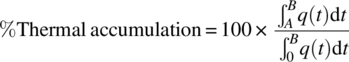
with t = 0 representing the time at which dosing starts, t = A the time at which dosing ends, and t = B the time at which all exothermicity has faded away (Figure 3.3). If the heat signal dropped to zero immediately after the dosing had stopped, there would be no thermal accumulation. On the other hand, if the dosing was instant (which is the case in a batch reaction), there would be 100% thermal accumulation.
FIGURE 3.3 Example of a reaction calorimetry experiment, indicating time 0 (start of dosing), time A (end of dosing) end time B (end of reaction) as they are used in the definition of thermal accumulation (Eq. 3.2).
Let us now take a closer look at the key figures that can be extracted from a calorimetry experiment and how they should be interpreted.
3.3.2.1 Reaction Heat–Adiabatic Temperature Rise– MTSR
The integration of the heat signal versus time gives us the total reaction heat, usually expressed in kJ or kcal. From this reaction heat, the adiabatic temperature rise of the synthesis reaction can be calculated according to Eq. (3.3):
where
- ΔHR: reaction enthalpy (kJ/kg)
- cp: specific heat capacity of the reaction mixture (kJ/kgK)
The MTSR can be calculated merely by adding the adiabatic temperature rise to the reaction temperature (Eq. 3.4):
Whereas the molar reaction enthalpy is an intrinsic property of a specific reaction, the adiabatic temperature rise is dependent on the reaction conditions. In the (hypothetical) example in Table 3.2, this difference is demonstrated.
TABLE 3.2 Theoretical Example of the Resulting Adiabatic Temperature Rise for the Hydrogenation of Nitrobenzene Under Different Reaction Conditions
| Case 1 | Case 2 | |
| Reaction heat | −560 kJ/mol | −560 kJ/mol |
| Concentration | 2 M | 0.5 M |
| Solvent | Chlorobenzene | Water |
| Density solvent | 1.11 kg/l | 1 kg/l |
| Specific heat solvent | 1.3 kJ/kg/K | 4.2 kJ/kg/K |
| ΔTad (Eq. 3.3) | 776 °C | 67 °C |
This example clearly shows the importance of reaction conditions, with the adiabatic temperature rise being more than 10 times higher in case 1. This dramatic difference can be fully attributed to the effect of the solvent acting as a heat sink. Working at higher dilution in a solvent with a higher heat capacity can drastically reduce the possible consequences of reaction that runs out of control. Unfortunately, running a process at higher dilution has an impact on the overall economy, so both aspects should be considered.
The adiabatic temperature rise is often used as a measure for the severity of a runaway reaction. A process with an adiabatic temperature rise of less than 50 K is usually considered to pose no serious safety concerns, at least when there is no pressure increase associated with the reaction. When a process has an adiabatic temperature rise of more than 200 K, a runaway reaction would most probably result in a true thermal explosion, and hence such processes require a very thorough safety study.
3.3.2.2 Thermal Accumulation
According to Eq. (3.2), the thermal accumulation can be calculated by the partial integration of the heat signal. Thermal accumulation is an important parameter in the assessment of the safety of a process. If a problem occurs during a process (cooling failure, stirrer failure, etc.), it is common practice to stop the addition of chemicals immediately. In case there is no thermal accumulation, the reaction will also stop immediately, and there will be no further heat generation that can lead to a temperature increase in the reactor. A reaction with 0% thermal accumulation is therefore called dosing controlled. If there is thermal accumulation however, part of the reaction heat will still be set free after the dosing has been stopped, and hence the temperature in the reactor can increase.
Because of the importance of the thermal accumulation, the MTSR is often specified as either being MTSRbatch or MTSRsemi‐batch. For the calculation of the former, the total adiabatic temperature rise is added to the reaction temperature, whereas, for the latter, the adiabatic temperature rise is first multiplied by the percentage of thermal accumulation. An example is given in Table 3.3.
TABLE 3.3 Example of the Effect of the Thermal Accumulation on the MTSRsemi‐batch
| Case 1 | Case 2 | |
| Reaction temperature (°C) | 60 | 60 |
| Total reaction enthalpy (kJ/kg) | −200 | −200 |
| Thermal accumulation (%) | 2 | 60 |
| Specific heat (J/gK) | 2 | 2 |
| ΔTad,batch (°C) | 100 | 100 |
| MTSRbatch (°C) | 160 | 160 |
| ΔTad,semi‐batch (°C) | 2 | 60 |
| MTSRsemi‐batch (°C) | 62 | 120 |
This example shows the big difference in intrinsic safety of the process between the two cases. Should a cooling failure occur in case 1, the temperature would never be able to rise significantly above the process temperature, provided of course that the dosing is stopped as soon as the failure occurs. In case 2, on the other hand, the temperature would increase to 120 °C without the possibility to cool, even when dosing is stopped immediately.
So, obviously, low thermal accumulation is to be preferred for any semi‐batch process. A high degree of thermal accumulation is a sign that the reaction rate is low relatively to the dosing rate. Two possible measures can be taken to decrease the thermal accumulation of a given process:
- Increase the reaction rate. This can be done by increasing the reaction temperature. Increasing the reaction rate means also increasing the heat rate of the reaction, so a calorimetry experiment at this new (higher) process temperature is required to make sure that the cooling of the reactor can cope with the heat generation under normal process conditions. Obviously, the increased temperature will lead to a smaller safety margin between reaction temperature and possible decomposition temperature, and this should be dealt with appropriately.
- Decrease the dosing rate.
3.3.2.3 Heat Rate
Whereas a correct determination of the total reaction heat is important, the rate at which this heat is being liberated is at least equally important for a proper safety study. Where a process is run under identical conditions both at large scale and in the calorimeter, the heat rate (in W/kg) is scale independent. It should be kept in mind, however, that the cooling capacity of a reaction calorimeter is in most cases several orders of magnitude higher than that of a large‐scale production vessel. A reaction calorimeter might still be able to keep a constant heat rate of 200 W/kg under control, running this process at production scale will most certainly lead to a runaway reaction. In such a case, the process should be redesigned as to decrease the heat rate, and ideally the calorimetry experiment should be repeated under the new process conditions to make sure that no unwanted side effects occur (higher thermal accumulation, sudden crystallization, formation of extra impurities, etc.).
Not only the absolute value of the heat rate has to be considered, the duration of the heat evolution is also important. A peak in the heat evolution that surpasses the available cooling capacity but which only lasts for a short period of time is not necessarily problematic. If such a peak is observed, one should calculate the corresponding adiabatic temperature rise and evaluate its consequences. E.g. a heat rate of 200 W/kg for two minutes would give rise to a temperature increase of 12 °C under adiabatic conditions, assuming a specific heat of 2 J/gK. If a cooling capacity of 50 W/kg is available, this will only be 9 °C. The issues one might encounter when scaling up a reaction to meet the heat removal capacities of the production vessel will be discussed in more detail.
3.3.3 Gas Evolution
Up until now, we have only focused on the heat being generated by exothermic chemical processes. From a safety perspective, gas evolution and a resulting pressure buildup can have even more devastating consequences, so proper knowledge of any gaseous products being formed during a process is crucial to assuring a safe execution at production scale.
There are quite a few common reactions that do liberate considerable amounts of gas: chlorinations with thionyl chloride, BOC deprotections, quenching of excess hydride, and decarboxylations, to name but a few. The most appropriate way to quantify the gas evolution during a reaction is to couple any type of gas flow measurement device to a reaction calorimeter and run the process under the same conditions as it will be run on scale.
There are several possibilities for the measurement of gas evolution at small scale:
- Thermal mass flow meters. This type of devices is probably the most widespread when a flow of gaseous products has to be measured. They are available in a large span of measuring ranges (from <1 ml/min to several thousand liters per minute), are relatively cheap, and deliver a signal that can be picked up easily as an input in the reaction calorimeter. However, this type of meters measures a mass flow (i.e. grams of gas per minute) and not a volumetric flow (milliliter per minute). When dealing with one known single type of gas, this is no problem since the volumetric flow can be easily calculated from the mass flow signal. When the gas to be measured is a mixture of different components, or when the composition of the gas stream is entirely unknown, the volumetric flow cannot be obtained reliably.
- Wet drum type flow meters. The gas is led through a drum that is half submerged in inert oil, causing this drum to rotate. This rotation is recorded and is proportional to the volumetric flow (as opposed to the thermal mass flow meters). When using a unit that is entirely made of an inert material (e.g. Teflon), a very broad range of gaseous products can be studied. However, the dynamic range of this type of instruments is only modest, accuracy at the low end of the flow ranges (0–20 ml/min) is rather limited, and the fact that the drum rotates in a chamber filled with inert oil makes it susceptible to mechanical wear. Although the oil in the gas meter is basically inert, most gasses are somewhat soluble in it, which can lead to a (small) underestimation of the gas flow in some cases.
- Gas burette. This type of device measures the pressure increase in a burette that is filled with inert oil, releasing the overpressure at a predefined value, making an accurate determination of low gas flow rates possible. The signal is proportional to the volumetric flow, the setup is extremely simple without any moving parts, and it is fully corrosion resistant (only glass and silicon oil in contact with the gas). However, the output signal is difficult to integrate in any evaluation software (combination of pressure signal and count of the number of “trips”), and the flow range that can be measured is limited at the high end to approximately 50 ml/min (using the standard type of burette).
- Rotameters, bubble flow meters, etc. There are different other types of laboratory gas flow meters that will not be discussed here since they give only a visual readout and not a signal that can be incorporated electronically.
- Some labs have developed in‐house solutions for the measurement of small gas streams. An example was published by Weisenburger et al. [11], where the gas stream from a small‐scale experiment is collected inside a gastight bag that is suspended in a closed bottle filled with ambient air. When gas fills the bag, air is pushed out of the bottle and passes through a thermal mass flow meter. This way, only air is passing through the meter, making proper calibration possible while also ensuring a better protection of the instrument when corrosive gasses are being measured. This system is only suitable for the measurement of small gas streams (limited to the size of the bottle and bag), and a fair degree of noise on the signal should be tolerated.
In the explanation above, it has been emphasized that the determination of a volumetric gas flow is of interest rather than a mass flow. When scaling up the reaction to plant scale, we need to make sure that all gas that is being produced can be removed safely from the vessel to the exhaust. This means that all of this gas will have to flow through piping with a certain diameter, and the limiting factor for a gas flowing through a pipe without causing pressure buildup is its volume and not its mass. The maximum allowable gas rate for a specific process depends on the actual production plant layout, and this will be dealt with in the next paragraph.
Apart from the obvious importance of measuring the gas flow rate during a process, it might also be of interest to characterize the gas that is being emitted. Although there is no difference in possible pressure buildup, having a release of 50 m3/h of carbon dioxide will obviously feel more comfortable for any chemist or operator than having a release of 50 m3/h of hydrogen cyanide. When gas evolution comes into play, industrial hygiene, environmental emission limitations, and hazard classification (e.g. when hydrogen is being set free) should all be addressed appropriately.
Characterization of the gas being liberated during a process at lab scale is not an easy thing to do. Ideally, an online mass spectrometer can be used to quantify the exact composition of the gas stream at any time. Mass spectrometers with an appropriate measuring range (down to 28 Da when carbon monoxide is to be detected), low dead volume to eliminate unnecessary long holdup times, and high resolution (both nitrogen and carbon monoxide have a molecular weight of 28; very high resolving power is needed to discriminate between them) do not come cheaply. Collecting the gas leaving the reactor in a gas sampling bag, and subsequently injecting this gas into a regular mass spectrometer can be a viable alternative. Another widely used technique is to trap the gas in a wash bottle with an appropriate solvent in which the gas either dissolves or with which it reacts and then to analyze this solution in a traditional way. Which technique is being used is irrelevant, but one should always try to know the composition of the gas stream leaving the reaction mixture.
3.4 SCALE‐UP OF THE DESIRED REACTION
3.4.1 Heat Removal
3.4.1.1 Film Theory
When designing an exothermic reaction for scale‐up, it is important to know what the heat removal capacity of the reactor at production scale is. Unfortunately this is easier said than done. The heat transfer between the heat transfer medium in the jacket and the reaction mixture is usually described in terms of a series of resistances, the so‐called film theory. It considers three main factors governing the heat transfer in a stirred tank reactor: the resistance of the inner film (boundary reaction mixture–vessel wall), the resistance of the vessel wall and the resistance of the outer film (boundary vessel wall–heat transfer fluid). This can be expressed numerically:
where
- U: overall heat transfer coefficient (W/m2K)
- hr: inner film transfer coefficient (W/m2K)
- d: thickness of the vessel wall (m)
- λ: thermal conductivity of the vessel wall (W/mK)
- hc: inner film transfer coefficient (W/m2K)
- Umax: maximum heat transfer coefficient (W/m2K)
From this equation, it can be understood that there are two main contributions to the overall heat transfer coefficient: one that is solely dependent on the characteristics of the reaction mixture and one that is solely dependent on the characteristics of the reactor. Indeed, the inner film transfer coefficient hr is a measure for the resistance to heat transfer between the reaction mixture and the vessel wall and is strongly correlated to the physicochemical properties of the reaction mixture (viscosity, density, heat capacity, etc.) and the stirring speed. Umax on the other hand can be interpreted as the maximum obtainable heat transfer coefficient in a certain reactor in the hypothetical case when the inner film resistance would approach zero. This term comprises of two contributing parts: one that is due to the thermal conductivity of the vessel wall and one that is due to the outer film coefficient. These two terms are solely dependent on the characteristics of the reactor.
This explains why a correct scale‐up of the heat transfer characteristics is so difficult: since U is dependent on both the process and the reactor, it ideally should be determined or calculated separately for each vessel–process combination. This is a rather time‐consuming process, as can be seen from the list actions that should be undertaken:
- Determine the Umax of the calorimeter at the process temperature.
- Determine U for the reaction mixture under process conditions in the calorimeter.
- From 1 and 2, calculate hr for the reaction mass in the calorimeter.
- Calculate hr for the reaction mass in the production vessel (literature scale‐up rules).
- Determine the Umax of the production vessel at the intended jacket temperature.
- From 4 and 5, calculate the according U‐value for the reaction mixture in the production vessel.
For a thorough description of the theory behind this approach, the reader should refer to the literature [12, 13]. In the following part, we will briefly discuss some major issues related to the determination of the heat transfer coefficient at production scale.
3.4.1.2 Determination of U
The most widely used approach to determine the heat transfer characteristics of a reactor is by means of the Wilson plot [14]. The heat transfer coefficient is determined experimentally (by means of a cooling curve) at several different stirring speeds. When plotting the reciprocal heat transfer coefficient at a certain jacket temperature versus the stirring speed to the power −2/3 (Eq. 3.6), a straight line is obtained, with the intercept being equal to ![]() .
.
where
- n = stirrer speed (in rpm)
- cte = constant.
An example of such a Wilson plot is shown in Figure 3.4.
FIGURE 3.4 Example of a Wilson plot for the determination of the heat transfer characteristics of a reactor. The markers are experimentally obtained heat transfer coefficients at different stirring speeds. Through these points a straight line can be fitted that yields the contribution of both the maximum heat transfer coefficient and the inner film coefficient to the total heat transfer coefficient.
This is intrinsically the most reliable way to determine the Umax for any reactor, since the result is independent of the solvent being used for the cooling experiment. When repeating the same experiments with a different solvent, the experimental points will differ, and the slope of the line will differ, but Umax will remain the same.
This method can be used for the characterization of a reaction calorimeter where a large number of either cooling curves or U determinations via the calibration heater can be run in an automated way. Since Umax is dependent on the filling degree and jacket temperature, a vast range of U determinations are necessary for a proper description of the heat transfer properties of the reaction calorimeter. It is our experience that isopropanol is the most suitable solvent for obtaining good Wilson plots in the reaction calorimeter.
This method can be applied to the reaction calorimeter in programmed mode, and it becomes rather cumbersome however for use at plant scale. Since each measuring point in the curve has to be obtained from 1 cooling curve at one stirring speed, it becomes very time‐consuming to gather the data needed for this plot. Therefore, another approach can be used for the estimation of Umax at production scale. As mentioned above, constructing the Wilson plot with different solvents will alter the slope but not the intercept. If water is used for the construction of the Wilson plot, the slope turns out to be very low, i.e. the contribution of 1/hr is low. This implies that determining the U‐value with a reactor filled with water at the highest possible stirring speed will yield a value that is close to Umax. This way, a good approximation of the maximum heat transfer capacity of the vessel can be obtained from only one experiment. This approximation will obviously be less accurate, but the error made is always on the safe side: the Umax will be underestimated, and hence in reality there will be more cooling power available than anticipated. An example of this approach is being shown in Figure 3.5, where the heat transfer coefficients for a typical stainless steel reactor and a glass‐lined reactor of 6000 L are shown as a function of jacket temperature for a filling degree of 50 and 85%. This shows clearly the large range of U‐values that can be encountered in practice.
FIGURE 3.5 Heat transfer coefficients for a 6000 L stainless steel and a 6000 L glass lined reactor. The reactor was filled with water for 50% of the nominal volume (thick line) or 85% (thin line), heated to the boiling point and then cooled to room temperature with a constant temperature difference between jacket and reactor of 20 °C at a high stirring speed. The heat transfer coefficient was determined as a function of the jacket temperature, and a curve was fitted through these data points to allow for extrapolation to other temperatures.
It is important to note that the Umax value is a function of the jacket temperature rather than the reactor temperature because it is linked to the properties of the jacket and vessel wall, which is always at approximately the same temperature as the jacket. This implies that cooling curves should be determined with a constant temperature difference between the jacket and reactor. If a cooling curve is recorded with the jacket constantly at its lowest temperature, the temperature dependence of the Umax is lost. Moreover, when calculating the final overall heat transfer coefficient of the reactor from its respective Umax value, the intended temperature offset between the reactor and jacket should be kept in mind. This is less of an issue in the reaction calorimeter, since the observed temperature differences between the jacket and reactor are usually a lot smaller than in a large‐scale reactor. Obviously, the values from Figure 3.5 apply only to the specific reactors in this specific plant, as different layouts in the cooling system, different materials of construction, different heat transfer media, and different temperature control strategies can all have a large influence on the heat transfer characteristics of a vessel.
3.4.1.3 Influence of the Inner Film Coefficient
Now that the Umax has been determined at both lab scale and production scale, let us turn our attention to the other term in Eq. (3.5), i.e. the inner film coefficient hr. This film coefficient is a measure for the resistance toward heat transfer between the reaction mass and the vessel wall. It is mainly governed by the stirring speed and the physical properties of the reaction mixture: a highly viscous reaction mixture will have more difficulties in dissipating reaction heat to the reactor wall than, for instance, pure water. Unfortunately enough, the influence of the inner film coefficient can be quite pronounced: if it were relatively small in comparison with the Umax term, it could be neglected, and one single heat transfer coefficient could be used for each vessel, irrespective of the reaction mixture.
When the Umax of the reaction calorimeter is known at the (jacket) temperature and fill degree used, the inner film coefficient can be calculated from the overall heat transfer coefficient as determined in the calibration procedure according to Eq. (3.5).
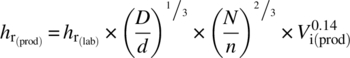
As the inner film coefficient is dependent on the mixing characteristics of the vessel used, it is scale dependent and should be scaled up accordingly. This is usually done according to Eq. (3.7):
where
-
 : the inner film coefficient at large scale
 -
 : the inner film coefficient at calorimeter scale
 - D: vessel diameter at large scale
- d: vessel diameter at calorimeter scale
- N: stirring speed at large scale
- n: stirring speed at calorimeter scale
-
 = viscosity number at large scale
The viscosity number is the ratio of the viscosity of the reaction mixture at the reaction temperature and its viscosity at the jacket temperature. When considering standard organic reactions in solution, this ratio is quite close to unity, so this factor is usually neglected. When studying polymerization reactions, however, this effect should be taken into account.
Using this equation, the inner film coefficient at production scale can be calculated, and hence the overall heat transfer coefficient is now known, according to Eq. (3.5). In order to get a more quantitative feeling for the influence of the different parameters on the overall heat transfer coefficient, let us take a look at a realistic numerical example.
TABLE 3.4 Example Problem 3.1 to Show the Influence of the Inner Film Coefficient on the Overall Heat Transfer Coefficient
| Calorimeter | Production Vessel | Calorimeter | Production Vessel | |
| Reactor temperature (°C) | 60 | 60 | 60 | 60 |
| Jacket temperature (°C) | ±60 | 20 | ±60 | 20 |
| Filling degree (%) | 50 | 50 | 50 | 50 |
| Umax at jacket temp (W/m2K) | 215 | 500 | 215 | 500 |
| Diameter reactor (m) | 0.12 | 2 | 0.12 | 2 |
| Stirring speed (rpm) | 450 | 100 | 450 | 100 |
| U experimental (W/m2K) | 180 | 120 | ||
| U calculated (W/m2K) | 337 | 169 |
The left part represents the case of a homogeneous nonviscous reaction mixture, the right part that of strongly heterogeneous reaction mixture. Bold values are the overall heat transfer coefficients for two different situations at lab and plant scale respectively.
3.4.1.4 Shortcuts to U‐Value Determinations
When the procedure for the determination of correct heat transfer data as described above is out of reach, there are other possibilities to make a rough estimation of the U‐values. If one chooses to go for these simplified estimation methods, care is needed to include a wide enough safety window when a batch is run for the first time in a certain reaction vessel.
A first possible estimation method is to simply use the heat transfer coefficient for a reactor filled with the neat solvent in which the reaction is to be performed. Cooling curves for some solvents are often readily available from cleaning campaigns. Since these cleaning cycles are usually repeated quite regularly, an indication of the evolution of the heat transfer characteristics of the reactor over time can also be obtained. It excludes the need for the separate determination of Umax with water, which is not often used as a cleaning solvent in a temperature cycle, and of the entire characterization of the Umax behavior of the reaction calorimeter. So if a reaction is to be run in a methanol solution at 30 °C, one could simply calculate the U‐value at that temperature from a cooling curve with neat methanol. This approach will yield acceptable results, as long as the reaction mixture is not strongly heterogeneous or highly viscous.
Another possible approach is to use very conservative general heat transfer coefficients in the scale‐up calculations. One could, for instance, record a cooling curve for methanol, calculate the U‐values from this curve, and then base all calculations on 50% of the heat transfer coefficient found. Although this method does not consider any specific effect of the physical properties of the reaction mixture on the heat transfer coefficient and should therefore only be used with great care and large safety margins, it can be an easy tool to give some guidance in the scale‐up calculations.
Again, it should be stressed that when the correct U‐values are not known and can only be roughly estimated, broad safety margins should be incorporated in the process, and the reactor data from the first batch should be checked carefully for any inconsistencies.
3.4.1.5 Practical Use of U‐Values
So now the U‐value of the reaction mixture at production scale has been determined, but what can we do with it? The main use of heat transfer coefficients is to allow for a correct calculation of dosing times, making sure that all heat that is being generated during the reaction can be safely removed. This is illustrated in the example below for a dosing controlled reaction. When dealing with a non‐dosing controlled reaction (i.e. with significant thermal accumulation), one should make sure that the available cooling capacity matches the heat release rate as observed in the calorimetry experiment at any time.
FIGURE 3.6 Influence of the heat transfer characteristics of a vessel on the dosing profile for an exothermic addition. The figure to the left shows the heat profile for a dosing controlled reaction in a vessel with a high heat transfer coefficient. The reaction mixture can be added relatively fast, since the cooling capacity is large. In the figure to the right, the same addition is shown in a reactor with a lower heat transfer coefficient. Less heat can be removed in the same period of time, hence the dosing has to be performed slower. The overall reaction heat (shaded area) is the same in both profiles.
3.4.2 Gas Evolution
3.4.2.1 Gas Speed
In the scale‐up of a process in which gas is being liberated, it is of utmost importance to make sure that all the gas that is set free can be evacuated from the reactor safely, without causing any pressure buildup. When a chemical plant is being designed, a certain layout for the scrubber lines is worked out. This specific layout implies that there is a maximum gas speed in the piping in order to avoid pressure buildup, entrainment of powders, or unintended changes in flow pattern or even flow direction. A maximum gas speed that is often used is 5 m/s. If the maximum design gas speed and the minimum diameter through which the gas has to pass are known, the resulting maximum gas flow can be calculated. Some typical piping sizes and the corresponding maximum gas flow to meet the 5 m/s criterion are given in Table 3.5.
TABLE 3.5 Influence of the Limiting Piping Diameter in the Scrubber Lines on the Maximum Allowable Gas Flow at Production Scale (Left) and the Corresponding Gas Flows at Lab‐ Scale (Right)
| Production Scale | Scale Down from 6000 L | |||||
| Diameter (cm) | Max flow (l/min) | Max Flow (m3/h) | 2 L Reactor Max Flow (ml/min) | 1 L Reactor Max Flow (ml/min) | 100 ml Reactor Max Flow (ml/min) | |
| DN25 | 2.5 | 295 | 18 | 98 | 49 | 5 |
| DN50 | 5 | 1 178 | 71 | 392 | 196 | 20 |
| DN100 | 10 | 4 712 | 283 | 1570 | 785 | 79 |
| DN150 | 15 | 10 603 | 636 | 3534 | 1767 | 177 |
These values assume that the installation is designed for a maximum gas speed of 5 m/s.
These figures clearly demonstrate the pronounced effect of the diameter of the narrowest piping the gas has to pass on its maximum flow rate: doubling the diameter allows a fourfold increase in gas flow.
The part of Table 3.5 shows some interesting scale‐down data. In these columns, we have calculated what the corresponding gas flow at lab scale is. For instance, if the narrowest piping in the scrubber line is a DN50, a maximum flow rate of 71 m3/h can be allowed at production scale. Using this maximum gas flow and assuming it concerns a 6000 L reactor, we can calculate the gas flow at lab scale. In this case, the corresponding gas flow in a 2 L reaction calorimeter would be 392 ml/min. This flow can be detected easily, but if the reaction is run in a 100 ml calorimeter, the corresponding gas flow is only 20 ml/min. One can imagine that such a low gas flow rate can be overseen easily during the process development work. This illustrates the importance of an accurate gas flow measurement combined with each reaction calorimetry experiment. Especially when small‐scale reactors are used (<1 L), care should be taken in choosing the appropriate gas flow measuring device.
These values for the maximum allowed gas flow apply mainly to the desired synthesis reaction. Exceeding this flow to a limited extent might result in operational problems such as slight pressure buildup, process gases entering a neighboring reactor that is connected to the same scrubber line, or suboptimal condenser and scrubber performance but will not necessarily lead to pronounced safety issues. When gas flow rates are considered an order of magnitude higher, vent sizing calculations come into play. This will be briefly discussed at the end of this chapter.
3.4.2.2 Reactive Gases
In the previous discussion, the only parameter of concern was the gas flow rate. In many cases, however, the gas being emitted is reactive by itself, and this can cause particular safety problems. One example of having a very high yielding but unfortunately enough undesired synthetic reaction is depicted in Scheme 3.1.
SCHEME 3.1 Example of two synthetic reactions that generate reactive gasses.
These two processes were both run in the same plant. By coincidence, they were being run at exactly the same time in two neighboring reactors. The reaction depicted at the top resulted in the emission of hydrogen chloride, while reaction at the bottom was releasing ammonia. Both reactors were connected to the same scrubber lines, and they inevitably reacted with each other, forming ammonium chloride in large amounts.
This solid material blocked the scrubber lines, and the reaction heat being evolved was large enough to partly melt the plastic scrubber lines. Fortunately enough there were no serious consequences, but this demonstrates the need for a broad safety overview in any chemical plant.
3.4.2.3 Environmental Issues
Although this factor is not related to process safety in the strict sense, the importance of the gas flow rate for environmental compliance should be mentioned here as well. It is important to know the layout of the gas treatment facility of the plant where the process is going to be run. If a carbon absorption bed is used, it is important to keep an overview of what the capacity of this bed is for the process gas being emitted: some gasses are retained better than others, and some gasses might even lead to dangerous hot spot formation in the bed. If a catalytic oxidation installation is used, it is important to know that some compounds (like hydrogen and alkenes) will lead to overheating in the installation if the flow is too high. And when no air treatment facility is installed at all, one should always make sure that the gas streams being emitted are within all environmental requirements. This assessment needs to be made for each production plant separately.
3.5 STUDYING THE DECOMPOSITION REACTION AT LAB SCALE
Having dealt with the study of the desired synthesis reaction (the first part of the cooling failure scenario), let us now turn our attention to the study of the undesired decomposition reaction. Decomposition reactions are of extreme importance for safety studies: in most cases the energies being released in decomposition reactions are several orders of magnitude higher than those being released in the synthetic reaction, and hence the possible consequences of decomposition reactions can be catastrophic. Prerequisites for any compound being used in a process include that, firstly, it should be stable at the storage temperature for at least the time span anticipated for storage under normal operational conditions. Secondly, it should be at least sufficiently stable at the process temperature being used. And finally, it is important to assess its stability at the MTSR as well, since this is a temperature that can be attained in case of a cooling failure during the process (see Figure 3.1). In this paragraph we will discuss how the thermal stability of reagents and reaction mixtures can be studied at lab scale and how these data can be used to ensure a safe scale‐up. But first we will start with another important characteristic of the stability of compounds, i.e. shock sensitivity.
3.5.1 Shock Sensitivity
Some compounds are known to be prone to explosive decomposition when subject to a sudden impact, and they are therefore called shock‐sensitive compounds. In this chapter we will refer to shock‐sensitive compounds as those products that are positive in impact testing via drop hammer. Any compound that has at least one of the following characteristics should be considered as possibly shock sensitive:
- The product has a very high decomposition energy (>1000 J/g).
- The product has at least one so‐called instable functional group.
- The product is a mixture of an oxidant and a reductant.
A list with some of the most common instable functional groups that can make a product shock sensitive is given in Table 3.6. Please note that this list is not exhaustive, and when in doubt the shock sensitivity of the compound should be tested [15].
TABLE 3.6 Non‐Exhaustive List of Functional Groups That Can Be Shock Sensitive
| Acetylenes | C≡C | Diazo | R=N=N |
| Nitroso | R─N=O | Nitro | R─NO2 |
| Nitrites | R─O─N=O | Nitrates | R─O─NO2 |
| Epoxides |  |
Fulminates | C≡N─O |
| N‐Metal derivative | R─N─M | Dimercuryimmonium Salt |
R─N=Hg=N─R |
| Nitroso | R─N─N=O | N‐Nitro | N─NO2 |
| Azo | R─N=N─R | Triazene | R─N=N─N─R |
| Peroxyacid | R─O─OH | Peroxides | R─O─O─R |
| Peroxide salts | R─O─O─M | Azide | R─N=N=N |
| Halo‐aryl metals | Ar─M─X | N‐Halogen compounds | N─X |
| N─O compounds | N─O | X─O compounds | R─O─X |
This list is extracted From Bretherick’s [9] (version 4).
When a compound is indeed shock sensitive, this may have serious consequences on the further development of the process, depending on the degree of shock sensitivity. There are restrictions for the transportation and storage of shock‐sensitive compounds, so getting permission to purchase and store any of these products can be cumbersome. Therefore it is vital to be aware of shock sensitivity issues at an early stage.
When a reagent used in a synthesis is known to be shock sensitive, this does not necessarily exclude it from being used. For instance, hydroxybenzotriazole (HOBT) is known to be shock sensitive in its anhydrous form but not in its hydrate form. Making sure that the appropriate grade of the chemical is used from an early stage on can therefore avoid many practical problems later on.
3.5.2 Screening of Thermal Stability with DSC
When evaluating the stability and risk potential of commonly used reagents, common literature and references such as safety data sheets (SDS) can be a good starting point. More often than not in the development of active pharmaceutical ingredients, the compounds used are entirely new so the necessary safety data must be produced experimentally. It is a good practice to start with thermal stability screening of newly synthesized compounds at a very early stage (when the first gram of product becomes available), since changes in the process chemistry are still possible without too much impact.
The most widely used technique for thermal stability studies is the DSC. In a DSC, a small cup with a few milligrams of product is heated at a predefined rate to a certain temperature. Typically, a sample could be heated from room temperature to 350 °C at 5 °C/min. During the heating phase, sensors detect any heat being generated (exothermic process) or absorbed (endothermic process) by the sample. The popularity of the DSC as a screening tool for thermal stability in process development is due to its low cost, wide availability of instruments from different suppliers, moderate experimental time (a typical run takes one to two hours), appropriate sensitivity (1–10 W/kg), and small sample size (1–50 mg).
A typical DSC run is shown in Figure 3.7. As can be seen in the graph, at temperatures below 75 °C, little thermal activity is observed. A first exothermic peak is observed at 110 °C, followed by a much larger exotherm exhibiting two peaks at around 225 and 270 °C. Integration of the entire exothermic signal yields a reaction enthalpy of more than 1000 J/g, indicating that this particular compound has a very high decomposition energy.

FIGURE 3.7 Example of a scanning DSC run of an unstable organic substance. The temperature was increased linearly from 30 to 350 °C and the subsequent heat signal was recorded (exotherm is shown as a positive, upward, signal).
When evaluating a DSC run, there are three main parameters of interest.
3.5.2.1 Reaction Enthalpy
Some typical decomposition energies for the most common thermally unstable groups are given in Table 3.7.
TABLE 3.7 Typical Decomposition Energies for Some Common Instable Functional Groups [2]
| Functional Group | ∆H (kJ/mol) | Functional Group | ∆H (kJ/mol) |
| Diazo ─N=N─ | −100 to −180 | Nitro ─NO2 | −310 to −360 |
| Diazonium salt ─N≡N+ | −160 to −180 | N‐hydroxide ─N─OH | −180 to −240 |
| Epoxide |
−70 to −100 | Nitrate ─O─NO2 | −400 to −480 |
| Isocyanate ─N=C=O | −50 to −75 | Peroxide ─C─O─O─C | −350 |
This table clearly shows that merely looking at a molecular structure can already give an indication about the decomposition potential of a reagent. Note however that the data in this table are given in kJ/mol, whereas DSC data are usually reported in J/g. The latter gives in fact a better indication of the intrinsic energy potential of the product, since the influence of an instable group will obviously be much larger in a small molecule than in a very large one. It is therefore no surprise that many of the most dangerous reagents (in terms of thermal stability) are indeed small molecules: hydroxylamine, nitromethane, cyanamide, methylisocyanate, hydrogen peroxide, diazomethane, ammonium nitrate, etc.
According to the observed decomposition enthalpy, a first assessment of the energy potential can be made. A decomposition energy of only 50 J/g is very unlikely to pose serious problems, even when the product would decompose entirely. On the other hand, a decomposition energy in the order of magnitude of 1000 J/g should be considered as problematic, and the first choice should always be to avoid the use of such chemicals as much as possible.
As already previously mentioned (Eq. 3.3), the reaction heat is directly proportional to the adiabatic temperature rise. For ∆Tad to be known, the cp of the compound or reaction mixture is needed. The heat capacity can be determined separately in the DSC, but in order to get a first indication, an estimated value can be used as well. Usually a cp of 2 J/gK can be used for organic solvents or dilute reaction mixtures, 3 J/gK for alcoholic reaction mixtures, 4 J/gK for aqueous solutions, and 1 J/gK for solids (conservative guess). A rough classification of severity of a decomposition reaction based on its reaction enthalpy and corresponding adiabatic temperature rise (in this case for cp = 2 J/gK) is given in Table 3.8.
TABLE 3.8 Classification of the Severity of Decomposition Reactions According to the Corresponding Adiabatic Temperature Rise
| ∆H (J/g) | ∆Tad (°C) | Severity |
| <−500 | >250 | High |
| −500 < ∆H < −50 | 25 < ∆Tad < 250 | Medium |
| >−50 | <25 | Low |
Assuming a cp of 2 J/gK.
One final remark should be made here about endothermic decompositions. Some compounds decompose endothermically, and whereas one might consider them therefore to be harmless, special attention for these compounds is sometimes needed. Decomposition reactions in which gaseous products are formed (such as elimination reactions) are often endothermic. The intrinsic risk of this type of decompositions lies therefore not in the thermal consequences but in a possible pressure buildup. For this type of compounds, an evaluation of the possible pressure buildup associated with the decomposition is recommended.
3.5.2.2 Onset Temperature
Even when a compound has a very high decomposition energy, it can still be possible to use it safely in a process, provided that the difference between the process temperature and the decomposition temperature is sufficiently high. The term “onset temperature” is used quite frequently to denote the temperature at which a reaction or decomposition starts. In reality, however, there is no such thing as an onset temperature, since the temperature at which a reaction starts is strongly dependent on the experimental conditions. The point from which on a deviation from the baseline signal can be observed is determined by the sensitivity of the instrument, the sample size, and the heating rate of the experiment. This implies that great care is needed when comparing “onset temperatures” obtained with different methods, but it does not completely rule out the use of this parameter in early safety assessment.
It should be mentioned here that the description above holds for the way in which the term “onset temperature” is usually interpreted in the process safety field. In other fields of research, the term onset is defined as the point where the tangent to the rising curve at the inclination point crosses the baseline. This definition is, e.g. used in the calibration of a DSC by measuring the melting point of a suitable metal (mostly indium). In this text, however, the term “onset” will always refer to the temperature at which a first deviation from the baseline signal is observed.
A rule of thumb that has been used quite extensively in the past is the so‐called 100 °C rule. This rule states that a process can be run safely when the operating process temperature is at least 100 °C below the observed onset temperature. This rule has been shown to be invalid in certain cases, so it should certainly not be used as a basis of safety. This does not mean however that it is completely useless. If a process is to be run on a relatively small scale (50 L or less) in a well‐stirred reaction vessel, natural heat losses to the environment are usually sufficiently large for the 100 °C rule to be valid. If the process is to be run at a larger scale, a proper and more detailed study of the decomposition kinetics (and especially of the TMRad) should be made, as will be discussed further on in this chapter. Here as well, it should be stressed that these remarks only apply to the thermal stability of the products, and extra care should be taken when gas evolution comes into play.
3.5.2.3 Reaction Type
When dealing with DSC data of compounds or reaction mixtures, merely looking at the shape of the peak can give some clues about the type of reaction taking place. The DSC run shown in Figure 3.7 consists of several different overlapping peaks, indicating a rather complex reaction type. Very sharp peaks are indicative for autocatalytic reactions, and extra care with this type of decompositions is needed [16].
Autocatalytic reactions are reactions in which the reaction product acts as a catalyst for the primary reaction. This implies that the reaction might run slowly at a certain temperature for a while, but as time passes more catalyst for the reaction is formed, and hence the reaction rate increases over time. Such reactions are therefore also called self‐accelerating reactions. This is in contrast with the more classical behavior of reactions following Arrhenius kinetics where the reaction rate stays constant (zero order) or decreases (first order or higher) with time at a certain temperature. Having determined the decomposition reaction in such a case on a fresh sample will therefore always give the worst‐case decomposition scenario, the initial rate measured will be the maximum rate for that sample at that particular temperature. This is not the case for autocatalytic reactions, where the reaction rate is strongly dependent on the thermal history of the sample. Measuring the reaction rate for a pristine sample might lead to an underestimation of the risk associated to the decomposition of this sample when it has been subject to a certain thermal history (e.g. prolonged residence time at higher temperature due to a process deviation). An example of an isothermal and a scanning DSC run for both an autocatalytic and a first‐order reaction are shown in Figure 3.8.
FIGURE 3.8 Example of a scanning DSC run (left) and an isothermal DSC run (right) of a reaction following nth order kinetics (thin line) and of an autocatalytic reaction (thick line).
As pointed out in the above, an autocatalytic reaction behavior is easily recognized by isothermal DSC experiments. If the temperature in the sample remains constant, the heat release over time will decrease in case of an nth‐order reaction but will show a distinct maximum in case of an autocatalytic reaction. Although not always as easy as in an isothermal DSC run, autocatalytic reactions can also be recognized in scanning DSC experiments where the peak shape is notably sharper than for nth‐order reactions. This is shown in Figure 3.8.
When a decomposition reaction is known to be autocatalytic, extra care is needed in order to avoid its triggering. For such compounds, any unnecessary residence time at elevated temperatures should be avoided. Extra testing might be appropriate to reflect the thermal history the product will experience at full production scale, since, e.g. heating and cooling phases may take considerably more time than in small‐scale experiments. It should also be kept in mind that temperature alarms are not always an efficient basis of safety for this type of decomposition reactions: since the temperature rise can be very sudden, this type of alarm might simply be too slow to ensure sufficient time is available to take corrective actions.
3.5.3 Screening of Thermal Stability: Pressure Buildup
As already mentioned earlier, in many cases the gas being released during a (decomposition) reaction can have greater safety consequences than merely the exothermicity. A proper testing method to determine whether a decomposition reaction is accompanied by the formation of a permanent (i.e. non‐condensable) gas is therefore very important.
There are several instruments commercially available that are suited for this type of testing. Generally speaking they consist of a sample cell of approximately 10 ml in which the sample is heated in a heating block or oven from ambient to around 300 °C. During this heating stage, the temperature inside the sample is measured, as well as the pressure inside the sample cell. The main criteria these instruments should meet are an appropriate temperature range (ideally from [sub] ambient to 300 °C), pressure range (up to 200 bar when measuring in metal test cells), and sample size (milligram to gram range). Some examples of such instruments available at the time of writing are the C80 from Setaram, the TSU from HEL, the RSD from THT, the mini‐autoclave from Kuhner, the Carius tube from Chilworth, and the Radex from Systag.
The most difficult aspect of interpreting the pressure data from this type of experiments lies in the differentiation between a pressure increase that is due to the formation of a permanent gas and a pressure increase due to an increased vapor pressure of the compounds at higher temperatures. When dealing with reaction mixtures in a solvent, the vapor pressure as a function of temperature can be calculated easily by means of the Antoine coefficients. These coefficients are readily available in the literature for most common solvents. If a plot of the vapor pressure as a function of the sample temperature matches the observed pressure profile, one can conclude that the observed pressure increase is due to the increased vapor pressure only. When in doubt or when the Antoine coefficients of the product are not known, e.g. when dealing with a newly synthesized product that is an oil, it is advised to run an isothermal experiment with pressure measurement at a temperature at which the decomposition is known or believed to occur at a considerable rate. If the pressure during this experiment remains constant, the pressure is due to vapor pressure, and if the pressure increases over time, it is due to the formation of a gaseous product. Alternatively, one could run two scanning experiments, each with a different filling degree in the test cell. If the pressure profile in the two runs match each other, the pressure is most likely to be due to vapor pressure, since it is not dependent on the free headspace available. If the test with the higher filling degree leads to a higher pressure, it is most likely to be due to the formation of a non‐condensable gas, since less headspace is available for a larger amount of gas, leading to higher pressure.
But why is it so important to differentiate between vapor pressure and the formation of a non‐condensable gas? If a certain pressure at elevated temperatures is only due to vapor pressure, it is relatively unlikely to pose problems. In such a case, a very rapid temperature increase is needed before the amount of vapor produced surpasses the amount that can be removed through the vent lines. When dealing with vent sizing calculations for serious runaway reactions, the effect of vapor pressure should definitely be taken into account. However, when dealing with moderate temperature rise rates, or in isothermal operation, vapor pressure is unlikely to lead to major problems. The story is entirely different for the formation of a permanent gas due to a (decomposition) reaction. In this case, each process parameter that leads to an increased reaction rate will lead to an increased pressure rise rate, with possibly devastating effects. Obviously, a temperature rise will lead to an increased reaction rate, but other effects such as an increase in concentration due to the evaporation of the solvent (e.g. in case of a condenser failure) or sudden mixing of two previously separated layers (e.g. switching the stirrer back on after a failure) could also lead to an increased pressure rise rate in the vessel. This is also important for storage conditions: vapor pressure in a closed drum will reach an equilibrium at a certain pressure, whereas the formation of a permanent gas will lead to a pressure increase over time and the subsequent possibility of rupturing the drum.
3.5.4 Adiabatic Calorimetry
When discussing the cooling failure scenario earlier in this chapter, the concept of adiabaticity was introduced. A system is said to be adiabatic when there is no heat exchange with the surroundings. In a jacketed semi‐batch reactor under normal process conditions, the reactor temperature is controlled by means of heat exchange between the reaction mixture and the heat transfer medium in the jacket. In case of a loss of cooling capacity (either because the heat transfer medium itself is no longer cooled or because it is no longer circulated), this heat exchange is no longer possible, and the reactor will behave adiabatically. This is considered to be the worst‐case situation in a reactor apart from a constant heat input (e.g. through an external fire), which will not be considered here.
For a lab chemist working on small‐scale experiments only, the concept of adiabatic behavior in a large vessel is often hard to imagine. “I did it in the lab and I didn't notice any exothermicity” is an often heard statement. However, heat losses at small scale are a lot higher than at large scale, so the heat generation should already be relatively high before it is noticed during normal synthesis work at lab scale. This can be seen in Table 3.9, where some heat losses for different types of equipment are listed.
TABLE 3.9 Typical Heat Losses for Different Types of Equipment [1]
| Heat Loss (W/kg/K) | Time for 1 °C Loss at 80 °C | |
| 5000 L reactor | 0.027 | 43 min |
| 2500 L reactor | 0.054 | 21 min |
| 100 ml beaker | 3.68 | 17 s |
| 10 ml test tube | 5.91 | 11 s |
| 1 L Dewar | 0.018 | 62 min |
This table shows the vast difference in heat losses between small scale and large scale and also the relevance of performing proper adiabatic tests. A 1 L Dewar calorimeter can be considered to be representative for other state‐of‐the‐art adiabatic calorimeters, and it can be seen that its heat losses compare favorably to reactors in the m3 range.
Since this adiabatic behavior is considered to be the worst‐case situation from a thermal point of view, it is of great interest to be able to mimic this situation in the lab under controlled conditions. An adiabatic calorimeter typically consists of a solid containment (to protect the operator against possible explosions that might take place inside the calorimeter) around a set of heaters in which the sample cell is placed. A thermocouple either inside the test cell or attached to the outside of the test cell records the sample temperature, and the heaters are kept at exactly the same temperature at any time in order to obtain fully adiabatic conditions. During the entire experiment, the pressure inside the test cell is recorded, as well as the sample temperature. The criteria an adiabatic calorimeter for safety studies should meet are obviously a high degree of adiabaticity (i.e. very low heat losses), an appropriate sample volume (typically between 5 and 50 ml), broad temperature range (ambient to 400 °C), high pressure resistance or a pressure compensation system (up to 200 bar), and high speed of temperature tracking (>20 °C/min). Some commercially available instruments are the ARC from Thermal Hazards Technologies, the Phi‐TEC from HEL, the Dewar system from Chilworth, and the VSP from Fauske. Several pharmaceutical and chemical companies have developed their own adiabatic testing equipment, mainly based on a high pressure Dewar vessel.
3.5.4.1 Adiabatic Temperature Profile
Let us consider the situation as being depicted in Figure 3.9. The reaction mixture is at a constant temperature of 120 °C when a cooling failure takes place. At this temperature, the reaction starts relatively slowly, and hence the temperature increases, albeit at a slow pace. Since most chemical reactions proceed faster at higher temperatures, the reaction rate (and thus the temperature rise rate) will increase as the reaction continues. This acceleration continues until finally the depletion of the reagents slows the reaction down again and a stable final temperature is achieved. The S‐shaped temperature curve seen in the graph is very characteristic for an adiabatic runaway reaction. As indicated on the graph, there are three main parameters that describe the process of a runaway reaction, i.e. the adiabatic temperature rise (ΔTad), the TMR, and the maximum self‐heat rate (max SHR). The first two have been discussed earlier in this chapter, and the max SHR is a measure for the maximum speed with which the reaction occurs and can be directly correlated to the power output of the reaction: a SHR of 1 °C/min corresponds to 33 W/kg reaction mixture for an organic medium with a cp of 2 and to 70 W/kg in aqueous medium

FIGURE 3.9 Typical adiabatic temperature versus time profile (left axis). The first derivative of the heat signal (self heat rate) is shown on the right axis. The TMR, adiabatic temperature rise (ΔTad) and the maximum selfheat rate (max SHR) are indicated.
This is important for vent sizing calculations and the assessment of using the boiling point as a safety barrier, as will be discussed further on in this chapter.
3.5.4.2 Heat–Wait–Search Procedure
The most commonly applied method for adiabatic testing is the so‐called heat–wait–search procedure, as depicted in Figure 3.10. In this procedure, the sample is introduced in the instrument at room temperature and then heated (heating step) to the starting temperature of the test. The sample is then allowed to equilibrate at this temperature (waiting step), followed by the so‐called search step. During this step (which usually takes between 5 and 30 minutes), the sample temperature is monitored to see if there is any sign of an exothermic reaction taking place. If the temperature rise rate under adiabatic conditions during this period is below the chosen detection threshold (typically 0.02 or 0.03 °C/min), the temperature is increased with a couple of degrees and the cycle starts all over again, until either an exotherm is detected or the preset final temperature has been reached. When an exotherm has been detected, the instrument will track the sample temperature adiabatically until the temperature rise rate drops below the threshold value (end of the reaction), after which the heat–wait–search cycle starts again. Alternatively, the run is aborted during an exotherm if the upper temperature limit of the experiment has been surpassed.
FIGURE 3.10 Typical representation of the heat‐wait‐search procedure in an adiabatic experiment. The sample is first heated to the desired temperature, then the temperature is allowed to stabilize during the wait period, and finally the temperature profile is checked for any sign of exothermicity during the search period. If exothermicity is detected, the temperature is adiabatically tracked until completion of the reaction or until the maximum experimental temperature has been reached. Otherwise the cycle is repeated.
Although adiabatic calorimeters can usually operate in other thermal modes as well, the heat–wait–search procedure is still the most widely used because it allows determining the onset temperature of the exotherm with great accuracy while keeping the experimental time acceptably short.
3.5.4.3 Thermal Inertia: φ‐Factor
As mentioned above, one of the main reasons why it is hard to extrapolate adiabatic behavior at large scale from small‐scale lab work is the dramatic difference in heat losses between these two working environments. There is another reason as well, which plays a very important role in the interpretation of adiabatic calorimetry, i.e. the thermal inertia or φ‐factor:
where
- mc: mass of the container (vessel or sample cell) (g)
- ms: mass of the reaction mass (g)
- cpc: heat capacity of the container (J/gK)
- cps: heat capacity of the reaction mass (J/gK)
When heat is generated in the reaction mixture, this heat will be used to increase the temperature of not only the reaction mixture itself but also the container, being the vessel at large scale or the test cell at small scale. The φ‐factor is therefore a measure of which fraction of the thermal mass of the entire system is due to the thermal mass of the reaction mixture and which part is due to the container.
In large‐scale equipment, the φ‐factor of a vessel during a runaway will be close to unity: i.e. the thermal mass of the vessel itself (mainly the jacket) will be low compared with the thermal mass of the reaction mixture (i.e. φ = 1). In small‐scale laboratory equipment, the φ‐factor is usually significantly higher than 1. In order to perform a lab scale experiment at a φ‐factor that is close to unity, one would need to use a very light test cell that can accommodate a large amount of sample. The influence of the φ‐factor on the runaway behavior of a system is very pronounced [17, 18], as can be seen in Figure 3.11. In this figure, the same adiabatic runaway profile is given for a sample being tested in two different test cells, one with a (hypothetical) φ‐factor of 1, the other one with a φ‐factor of 2 (simulations). As can be seen, the curves differ drastically. In every aspect, the curve obtained with φ = 1 is by far more severe than the one obtained with φ = 2. The total adiabatic temperature rise scales linearly with φ, i.e. the observed ΔTad in a φ = 2 experiment will be exactly half of the ΔTad in a φ = 1 experiment:
FIGURE 3.11 Influence of the φ‐factor on the adiabatic temperature profile [16]. The figure to the left represents an adiabatic experiment on exactly the same sample, but once measured at a φ = 1 and once at φ = 2. The influence of the thermal inertia on the result is pronounced. This difference is even larger in the case of two consecutive reactions, as shown in the figure to the right.
Source: Reprinted with permission from Dermaut [17]. Copyright 2006 American Chemical Society.
The TMR scales almost linearly with φ in most cases, but the max SHR scales far from linear with φ. The max SHR in an experiment with φ = 1 can easily be 10 times higher than in the φ = 2 experiment! The numerical data for the curves as depicted in Figure 3.11 are given in Table 3.10.
TABLE 3.10 Key Figures for the Adiabatic Runaway Profile from Figure 3.11
| Φ = 2 | Φ = 1 | |
| ΔTad | 70 °C | 140 °C |
| TMRad | 50 min | 90 min |
| Max SHR | 0.8 °C/min | 4.5 °C/min |
These data show that the adiabatic temperature rise scales linearly with φ. The TMRad scales approximately linearly with φ, whereas the max SHR does not.
Figure 3.11 also gives the runaway behavior of one reaction in a test cell with a (hypothetical) φ‐factor of 1 as compared with the same run in test cell with a φ‐factor of 2. In this case, however, the difference between the two runs is even more pronounced. The reaction consists of two consecutive reactions, and running this reaction at φ = 1 will result in a temperature profile where the first exotherm continues into the second one, leading to a very rapid temperature rise. In the run with φ = 2, the temperature rise from the first exotherm will be far less pronounced, and this will lead to a significant time interval between the two exotherms. Hence the severity of this run will be significantly lower than that of the run with φ = 1.
These two examples show the importance of the φ‐factor on the experimental results. Ideally one would try to perform the adiabatic measurement in a low φ test cell. In many cases this is difficult to obtain experimentally, and a proper extrapolation to low‐φ conditions is needed.
3.5.4.4 Interpretation of Adiabatic Experiments
Adiabatic experiments can be performed for different reasons, but usually the main goal is to get a representative idea of what the temperature and pressure profile could be in a full‐scale reactor in case of a runaway reaction. If the adiabatic experiment is performed at a φ‐factor close to unity, the match between the two will indeed be close. Let us take a look at the most important parameters to analyze.
- Adiabatic temperature rise. This value can be directly extracted from the thermal profile. When dealing with very violent reactions, it is probably not possible to obtain the total adiabatic temperature rise as the maximum safety temperature or pressure of the equipment will be surpassed and the experiment will be automatically stopped. This is not necessarily a problem since ΔTad can be obtained from other experiments as well (e.g. from DSC), and for this type of violent reactions, the temperature profile close to the onset temperature is far more important. Whether the final temperature would be 1000 or 700 °C is relatively unimportant, it will be a full‐blown thermal explosion anyhow. It should be kept in mind that the observed ΔTad should be multiplied with the φ‐factor in order to obtain the correct adiabatic temperature rise in case of a large‐scale runaway (Eq. 3.9).
- Onset of the exotherm. Here as well, the term onset refers to the point where deviation from the baseline can be observed and is hence instrument dependent. In adiabatic calorimetry a detection threshold of 0.02 °C/min is often used, which corresponds to a 1.4 W/kg in case of an aqueous reaction medium. Referring to Table 3.9, we know that the natural heat loss of a 5000 L reactor at 80 °C and an ambient temperature of 20 °C is 1.6 W/kg. These two figures match quite closely, so the temperature at which the exotherm is detected in the adiabatic calorimeter with this sensitivity is most likely to be the temperature at which exothermicity will be first noticed under adiabatic conditions at large scale (at least for temperatures higher than 80 °C). If the onset temperature is well above the MTSR, the decomposition is unlikely to be triggered, even in case of a cooling failure during the synthesis reaction. If the onset temperature is close to the MTSR, a calculation of the TMRad should be made, as will be discussed further on.
- Pressure profile. A careful analysis of the pressure profile should be made after each experiment. Very often, the pressure signal will be more sensitive to detect the start of a decomposition reaction than the temperature signal [19]. If a slow pressure increase during any of the search periods is observed, a decomposition reaction with gas evolution should be suspected. Some software packages allow for a direct overlay of the vapor pressure of any chosen solvent related to the sample temperature. This can be very indicative to discern between permanent gas formation and vapor pressure. If this is not possible, looking at the pressure profile during the wait and search period should yield the same information: if the pressure remains constant during this stage (when the sample is at a constant temperature), vapor pressure is the most important contribution to the overall pressure. If the pressure rises during this stage, formation of a permanent gas is most likely to happen. If the pressure drops at a certain point, a leak of the test cell has most probably occurred.
- Self‐heat rate (temperature rise rate). The temperature rise rate of a runaway reaction can be calculated by taking the first derivative of the temperature versus time plot. Two things should be kept in mind when analyzing the SHR: firstly the dramatic influence of the φ‐factor on the SHR, as discussed above, and secondly the fact that the associated pressure rise rate can have far more serious consequences. So in case the SHR is low at any time (e.g. below 2°C/min) in a low‐φ experiment (φ < 1.2) and there is no strong pressure increase, the consequences of the runaway reaction are unlikely to be severe.
- Pressure rise rate. The analysis of the pressure rise rate data is far from trivial. First thing to keep in mind is the influence the free headspace volume in the adiabatic calorimeter has on the finally observed pressure profile. If a permanent gas is being formed during the runaway reaction, the observed pressure increase will be considerably larger when the test has been performed with a small free headspace (e.g. a filling degree of 90% of the test cell) than in the case of a large free headspace (e.g. 50% filling degree). Therefore, it is advisable to use a ratio reaction mixture versus free headspace that is comparable with the situation at a large scale. As mentioned before, this is only relevant when dealing with the formation of a permanent gas, not when considering vapor pressure data. Moreover, as the pressure rise rate is in any case directly correlated to the temperature rise rate, the remarks made in the point above about the influence of the φ‐factor hold here as well. The pressure rise rate can be calculated back to a gas evolution rate (see also the Example Problem 3.3), and if the thus obtained gas flow is below the design limits of the installation under normal process conditions, no problems are to be expected. If this limit is exceeded to a limited extent, some operational issues can be suspected (limited condenser capacity, disturbed flow patterns in the venting line, etc.) without serious safety consequences. If the gas flow rate is considerably above this design limit, proper vent sizing calculations are needed to make sure that the emergency relief system is sufficient to cope with a runaway reaction. This point will be briefly discussed in a later paragraph.
Let us now consider a real‐life example of such an adiabatic experiment. In Figure 3.12, a heat–wait–search experiment of a relatively concentrated solution of dibenzoyl peroxide in chlorobenzene is shown. The experiment was conducted in glass test cell with a φ‐factor of 1.5.

FIGURE 3.12 Adiabatic heat‐wait‐search experiment on a 0.75 M solution of dibenzoylperoxide in chlorobenzene. The test was conducted in a glass test cell with a φ‐factor of 1.5. Exothermicity is observed at 58 °C, the run is aborted at 200 °C in order to prevent leaking of the silicone septa used to close the test cell [16].
A close inspection of the temperature profile indicates that the thermal activity starts already at 45 °C, but the detection threshold of 0.02 °C/min is only reached at 58 °C. At this temperature the instrument goes into tracking mode, and a max SHR of more than 40 °C/min is reached after 280 minutes. The observed adiabatic temperature rise is 140 °C, but in reality it will be higher since the run was aborted at 200 °C in order to prevent leakage of the silicone septa used to seal the glass test cell. An overlay of the vapor pressure curve with the pressure profile shows that a large part of the observed pressure is due to gas evolution of the decomposition reaction. The maximum pressure rise rate is very high, more than 200 bar/min. Keeping in mind that this experiment was conducted at a relatively high φ‐factor, it is clear that the severity of this runaway is totally unacceptable for introduction at a large scale. An obvious safety advice would be to investigate the use of a more dilute solution of this compound, or to turn to other, more stable reagents.
3.5.4.5 Using the Boiling Point as a Safety Barrier
When a runaway reaction takes place in a reactor, the temperature of the reaction mixture can reach the boiling point. This can either be an extra risk that needs to be taken into account or it can act as an efficient safety barrier [20].
If the heat rate under adiabatic conditions at the boiling point is low, part of the solvent will be evaporated, but the temperature will remain constant, and this will temper the runaway reaction. When the detected onset temperature in the adiabatic calorimeter is close to the boiling point, this can be a very effective safety barrier.
If the heat rate at the boiling point is relatively high, other effects might come into play:
- Evaporation of the solvent. If the boiling point is reached, part of the solvent will start to evaporate. This in itself will have a cooling effect, but when the vapor is no longer condensed and returned to the reactor, the reaction mixture will become more concentrated. This in turn will lead to an increased reaction rate and also to an increased boiling temperature. This should be taken into account when relying on the reflux barrier as a basis of safety.
- Swelling of the reaction mass. If the reaction mixture starts to boil vigorously, a kind of “champagne effect” may take place, leading to an increase of the volume of the reaction mass. In such a case the reactor content might even be forced out of the reactor into the condenser and scrubber lines.
- Flooding of the vapor line. This effect will occur particularly when countercurrent condensers are used (i.e. the vapor and the condensate flow in opposite direction through the condenser). If the vapor flow through the condenser is too high, this flow will prevent the condensed liquid to flow back into the reactor, and this liquid will be carried along with the vapor flow. Here as well, solvent will enter the scrubber lines with all possible problems associated with it.
Provided that all of the abovementioned factors are taken into account, the reflux barrier can be used as a very effective safety barrier. For a more quantitative description, the reader is referred to the literature [3].
3.5.5 TMRad Calculations
In the discussion of the cooling failure scenario, the importance of the temperature at which the TMRad is 24 hours was pointed out. It was stated that if the TMRad at the MTSR is more than 24 hours, the reaction can be considered to be safe. This obviously implies a correct determination of this important parameter. Several approaches can be followed to do this, each with their merits and shortcomings.
3.5.5.1 Determination from 1 DSC Run
A first approximation of the temperature at which the TMRad is 24 hours (we will call this temperature TMRad,24h) can be made from one single DSC run. A full discussion of the theory behind this approach is out of scope here, so the reader is referred to the original publication by Keller et al. [18]. We will however point out the basic concept with an example.
The idea behind this approach is quite simple: measure the heat release at one temperature, and assume that the reaction follows zero‐order reaction kinetics with a low activation energy of 50 kJ/mol. From this, the heat release at any temperature and hence the TMRad,24h can be calculated. The assumptions on which this approach is based and the practical calculations are discussed below.
- Zero‐order assumption. A “classical” behavior for a reaction is that it follows nth‐order Arrhenius kinetics. This means that the reaction rate increases with concentration and temperature. This implies that the reaction rate will decrease over time when the reaction temperature is constant (see Figure 3.8) as the concentration of the reagents drops with increasing conversion. In a reaction that follows zero‐order kinetics, however, the reaction rate is independent of the concentration. This means that the reaction rate remains constant at a given temperature from the start (0% conversion) until the end (full conversion) of the reaction. Assuming this type of reaction kinetics leaves out the concentration dependence and makes the calculations a lot easier. It should be kept in mind however that this is an assumption; in reality the reaction is most likely not going to follow these kinetics. It is however a “safe” assumption, since the reaction rate will be overestimated as the decrease in reaction rate with decreasing reagent concentration is neglected. The fact that this is indeed a “worst‐case” assumption is discussed thoroughly in the original publication.
- Low activation energy. The dependence of the reaction rate on the temperature is dictated by the activation energy: the decrease in reaction rate when lowering the reaction temperature is more pronounced for a reaction with high activation energy than for a reaction with a low activation energy. Since we will try to extrapolate the reaction rate at lower temperatures from one single measurement at one temperature, the activation energy needs to be known or estimated. A correct determination of the activation energy is possible by means of DSC, but not always straightforward. Therefore, the activation energy is assumed to be 50 kJ/mol, which is very low for organic reactions and decompositions. Choosing a low activation energy will again be on the safe side, since it will tend to overestimate the reaction rate at lower temperatures.
- Determination of the reaction rate (heat rate) at one temperature. A correct determination of the heat rate at one temperature is needed, preferably in a relatively early stage of the reaction since this will minimize the error introduced by the zero‐order assumption. The heat signal should be well separated from the baseline, however, in order to obtain an accurate signal. Keller et al. suggest to search for the temperature at which the heat rate is 20 W/kg. This is a sensitivity that is well within reach of any decent DSC apparatus. In the example shown in Figure 3.13, this heat rate is observed at 111 °C.
- The heat rate at other temperatures can now be calculated according to Eq. (3.10):
where
- q0: heat rate at the new temperature
- qonset: heat rate at the onset temperature (in this case 20 W/kg)
- Ea: activation energy (50 kJ/mol)
- R: universal gas constant (8.31 J/mol K)
- Tonset: onset temperature (in this case 111 °C or 384 K)
- T0: new temperature at which the heat rate is to be calculated
- From this, the TMRad can be calculated for any temperature according to
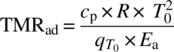

FIGURE 3.13 Example of a scanning DSC run of a highly unstable organic compound. The figure to the left shows the entire run, the figure to the right is zoomed in on the start of the exotherm.
If this calculation is performed for a number of temperatures, TMRad,24h can be determined, as shown in Table 3.11.
TABLE 3.11 Extrapolation of the Heat Rate and TMR of the DSC Signal from Figure 3.13 to Lower Temperatures
| T0 (°C) | q0 (W/kg) | TMRad (h) |
| 111 | 20 | 0.7 |
| 101 | 13.2 | 1 |
| 91 | 8.5 | 1.4 |
| 81 | 5.3 | 2.2 |
| 71 | 3.2 | 3.4 |
| 61 | 1.9 | 5.4 |
| 51 | 1.1 | 8.8 |
| 41 | 0.6 | 14.9 |
| 31 | 0.3 | 26.2 |
In this example (using a cp of 2 kJ/kgK), the TMRad,24h is estimated to be 31 °C. Another interesting point we can learn from this table is that a heat release of only 10 W/kg corresponds to a TRMad of less than one hour!
This example shows how the TMRad,24h can be extrapolated from only one DSC experiment. Because of the assumptions made, this will only be a rough estimate that can differ considerably from the true TMRad,24h. The merit of this method however lies in the fact that all assumptions are on the safe (conservative) side. If the thus obtained TMRad at the MTSR is longer than 24 hours, no further testing is needed. If it is shorter than 24 hours, a more accurate determination of the TMRad,24h might be needed, as will be discussed below.
One final remark is needed about autocatalytic reactions. Since the thermal history of a sample is so important in the characterization of autocatalytic (decomposition) reactions, their TMRad is much harder to determine. The method described here should therefore not be used for this type of reactions, and more elaborate adiabatic testing will be needed.
3.5.5.2 TMRad from 1 Adiabatic Experiment
Probably the best way to determine the TMRad,24h accurately is to perform a number of adiabatic experiments in a low‐φ test cell, each at a different starting temperature, and then determine the TMR for each of these experiments until the temperature at which this TMR is 24 hours is found. Obviously, this will be a very time‐consuming procedure, and better alternatives are to be sought for. It would be beneficial if we could extract a reliable TMRad,24h from one single adiabatic heat–wait–search experiment at a somewhat higher φ‐factor. This way, we would run an experiment under adiabatic conditions, which is closer to the real situation in a vessel during a runaway reaction than a scanning DSC experiment. Also, if we can run in HWS mode, the experimental time will be reduced significantly, and running at a higher φ‐factor (e.g. 1.5) is experimentally easier than at a φ‐factor close to unity. The question is how to extrapolate the data from this single adiabatic experiment to other temperatures and other φ‐factors.
In one of the classical papers about adiabatic calorimetry, Townsend and Tou [21] evaluated in great detail the analysis of experimental adiabatic data. In this article, they present a method to extrapolate the experimental TMR to other temperatures and other φ‐factors. A full description of the kinetic evaluation made in the original paper is out of scope here, but the general concepts and the practical use of this approach are discussed below.
We start from an adiabatic experiment, where we can determine the TMR at the onset temperature directly from the temperature versus time plot. The first extrapolation to be made is from the experimental φ‐factor (i.e. >1) to the “ideal” case of φ = 1. Townsend and Tou state that for most relevant decomposition reaction with a high activation energy, the TMR scales linearly with φ (Eq. 3.12):
Moreover, a method is described to extrapolate TMR data to lower temperatures as well. Assuming the reaction follows zero‐order kinetics, it can be shown that there is a linear correlation between the logarithm of the TMR and the inverse temperature according to Eq. 3.13:
Hence plotting the logarithm of the TMR versus the inverse temperature will yield a straight line with a slope proportional to the activation energy and the intercept being equal to the logarithm of the frequency factor.
Using these two equations, the TMRad,24h can be determined if the TMRad is known at a number of different temperatures. Since the approach is partly based on zero‐order assumptions, it is important to focus on the early part of the exotherm, since the influence of a decrease in concentration due to conversion can be neglected there. This way, the experimentally obtained TMRad at the onset temperature and at a couple of temperatures that are slightly higher are determined. These values are then corrected for the experimental φ‐factor according to Eq. (3.12). Finally a straight line is fitted through the plot of ln(TMRad) versus 1/T, and the point at which the TMRad is equal to 24 hours can be read from the graph. This approach is illustrated in the example below.
Let us consider the adiabatic experiment as represented in Figure 3.12. The φ‐factor used in this experiment was 1.5. The onset of the exothermicity is detected at 58 °C, 146 minutes after the start of the experiment. The maximum rate is reached after 429 minutes; hence the TMRad at this temperature is 283 minutes. We will consider the TMR at five different points in the early part of the exotherm, i.e. at 58, 60, 62, 64, and 66 °C. The corresponding TMRad at the experimental φ‐factor and at φ = 1 are calculated, as shown in Table 3.12.
TABLE 3.12 TMR at Different Temperatures from the Experimental Adiabatic Run as Shown in Figure 3.12
| Temperature (°C) | Time (min) | TMRad (min) | |
| Φ = 1.5 | Φ = 1 | ||
| 58 | 146 | 283 | 189 |
| 60 | 189 | 240 | 160 |
| 62 | 230 | 199 | 133 |
| 64 | 265 | 164 | 109 |
| 66 | 294 | 134 | 90 |
The TMRad at φ = 1 is calculated according to Eq. (3.12).
The according plot based on these data is shown in Figure 3.14. It can be seen that the correlation is indeed linear for both experimental and φ‐corrected data points. From the graph, the TMRad,24h can be obtained directly. In this case, the TMR will be 24 hours at 38.3 °C.
FIGURE 3.14 Extrapolation of the experimentally obtained TMR to lower temperatures and to φ = 1. The triangles represent the experimentally obtained TMR data at φ = 1.5, the squares are the corresponding calculated data at φ = 1, and the TMRad,24h can be read from the graph as indicated by the arrows.
The advantage of this method over the above method based on one DSC measurement is the increased accuracy. The reason for this can be found in different aspects of this approach:
- This method is based on an adiabatic experiment that will be by definition more representative for the situation in a large‐scale reactor during a runaway reaction than a DSC experiment.
- The temperature range over which the extrapolation takes place is fairly limited: in our example the difference between the experimental onset temperature and the finally obtained TMRad,24h is only 20 °C (as compared with 80 °C in the DSC example).
- The extrapolation for the φ‐correction is also limited (from φ = 1.5 to φ = 1).
- By using only data points in the early part of the reaction, the error introduced by assuming zero‐order kinetics is limited. Indeed, in this early stage with low conversion, the concentration of the reagents can be assumed to be constant.
Also for this method of determining TMRad,24h, a word of caution is needed. Only the data points in the early part of the exotherm are used; consequently we are dealing with very low heat rates at that moment. This poses high demands on the quality of the experimental data: a small amount of drift in the temperature stability of the instrument (either positive or negative drift) can have a profound effect on the final result. It is our experience that a well‐operated adiabatic calorimeter should be able to deliver reliable results, provided that regular drift checks on empty test cells are performed to confirm the stability of the instrument.
Here as well, extra attention is needed when dealing with strongly autocatalytic reactions, since this method might overestimate the TMRad for that kind of reactions, leading to unsafe extrapolations. When a very sudden and sharp temperature increase is noticed in an adiabatic experiment, autocatalysis should be suspected, and more testing will be appropriate. When in doubt, an iso‐aging experiment at a temperature close to the calculated TMRad,24h should be conducted to check the validity of the calculations.
3.5.5.3 Kinetic Modeling
Both of the abovementioned methods make it possible to extract the TMRad,24h from one single experiment but with a limited accuracy due to the assumptions made. There are more advanced methods available as well, which ask for a larger number of experiments and more advanced mathematical models, but which lead to more accurate description of the reaction and allow for a broader range of simulations.
One possible approach to kinetic modeling is the fully mechanistic description of the reaction, which implies a complete understanding of the (decomposition) reaction at a molecular level. The reaction is therefore split up into its elementary reactions, and for each of those the frequency factor, reaction order and activation energy are determined. It goes without saying that not only is this method quite elaborate from an experimental and computational point of view, but it also enables the widest range of process conditions that can be simulated (different concentrations, temperatures, φ‐factor, etc.) [22, 23]. This type of modeling is usually applied to the desired chemical reaction and less often to the undesired decomposition reactions.
Another possibility is the so‐called nonparametric kinetic modeling. In this approach, a general kinetic model of the (decomposition) reaction is constructed based on a number (usually 5) of DSC experiments with different heating rates [24, 25]. This kinetic description is said to be model free, meaning that there are no explicit assumptions being made about the reaction type. This type of modeling can lead to an accurate description of the reaction and enables the simulation of any temperature profile for the sample studied. With advancements both in readily available computing power and in fundamental understanding of the underlying theoretical kinetic models, this type of modeling is becoming more widespread and has even reached a point where some large companies tend to prefer modeling over adiabatic testing. It is worth pointing out however that, in order to guarantee a safe process development, the combination of data from different sources (modeling and experimental isothermal, non‐isothermal, and adiabatic data) is the preferred way to get to a fundamental understanding of a process during intended, non‐intended, and storage conditions.
The reader is referred to the literature for a more detailed discussion of the different possibilities of kinetic modeling for both safety studies and process development [23, 24, 26–28].
3.6 REACTIVE WASTE
In the past decades, knowledge and awareness with regard to reactive chemistry hazards have increased considerably both in industry and academia. One aspect of chemical reactive hazards that is still often overlooked and causes incidents on a regular basis is related to waste streams. When designing a chemical process, be it in the lab or in a production plant, one has to keep the reactivity of all chemicals in mind “from cradle to grave.” When using excess reagents, reactivity does not magically disappear once poured into the waste container.
There are several reasons why waste streams can cause unexpected safety issues:
- Incomplete understanding of the mass balance of the process and waste streams. When considering process safety, one has to keep in mind the entire mass balance of all products, including waste streams. By‐products that are formed should always be kept in mind (e.g. triethylammonium hydrochloride when capturing HCl formed in the process) since they may cause compatibility issues further downstream. The same holds for any excess reagents being used. An exact knowledge of the content of all streams involved in the process is key to assure a safe execution in the plant.
- Variability in storage conditions. During the reactive phase of a process, important factors like temperature and reaction time are usually very well known and controlled, and the safe limits are described and analyzed. For waste streams, this is very often not the case. The time during which a certain waste stream is stored (either on‐site or off‐site at the waste treatment facility) is usually ill‐defined. Storage conditions can vary as well, with temperatures ranging from as low as −10 °C in wintertime to 40 °C or more in summertime. To complicate things even further, these storage conditions are usually not being monitored or logged. These varying conditions make it more challenging to assure the safe handling of these waste streams.
- Mixing with other streams. In many cases, waste streams from one process are mixed with those of other processes. Generally speaking, it is very hard to know in advance which other chemicals a certain waste stream may be exposed to. Therefore, one has to consider all reactivity left in a certain waste stream and neutralize those where it is appropriate.
- Transfer between sites. Most companies send their waste streams to other companies for final disposal and/or treatment. Therefore the knowledge of the exact composition is very limited at the receiving end of this process, making it difficult to anticipate any reactivity hazards.
It is clear that the points above should be a warning to have a closer look at the waste streams involved in each process. Some examples of possible reactive waste incidents are briefly discussed:
- Water reactive chemicals. As a basic rule, all waste streams containing water reactive reagents should be decomposed in a controlled manner before further mixing. Certainly when the reaction with water gives rise to gas generation (which is often the case, like with thionyl chloride, oxalyl chloride, isocyanates, hydrides, etc.), since the presence of water in mixed waste streams can never be ruled out completely. Even a stoichiometric excess of as little as a couple of mole percent should always be decomposed under controlled conditions, since relatively small and slow gas release rates can lead to dangerous pressure buildup in a closed container. Also when the reaction with water does not give rise to gas generation, care is needed. When using acetic anhydride as a solvent, one has to keep in mind that it will react in an autocatalytic manner with water and alcohols, releasing a significant amount of heat during this process. Therefore even this relatively common solvent deserves further attention when dealing with waste streams. It is also noteworthy that most water‐reactive chemicals also react with alcohols, adding further to the risk of encountering unwanted side reactions when poured down the waste.
- Strong acids. Many synthetic reactions are acid catalyzed, so a multitude of unwanted reactions can be expected when adding strong acids to a waste stream. Most chemical waste treatment facilities do not accept strongly acidic waste streams to start with, so in many cases they should be neutralized before mixing with other streams or be collected and disposed of separately.
- Nitric acid. Nitric acid deserves a special place, as the description in Bretherick's justifies [9]: “…Nitric acid is the common chemical most frequently involved in reactive incidents, and this is a reflection of its exceptional ability to function as an effective oxidant even under fairly dilute conditions (unlike sulfuric acid) or an ambient temperature (unlike perchloric acid). Its other notable ability to oxidize most organic compounds to gaseous carbon dioxide, coupled with its own reduction to gaseous ‘nitrous fume’ has been involved in many incidents in which closed, or nearly closed reaction vessels or storage cabinets have failed from internal gas pressure.” Chemical reactivity incidents involving nitric acid still occur all too frequently, in a study from Etchells et al., and it was shown that from the 142 incidents reported to HSE between 1989 and 2005, 14% of them were related to nitric acid reactivity [29].
- Intrinsically unstable reagents. Some reagents are inherently unstable and can therefore pose a safety risk when ending up in waste streams. Typical examples are hydrogen peroxide (gas formation upon thermal decomposition) or hydroxylamines (exothermic decomposition, strongly influenced by contamination with metal ions). When such reagents are used in a process, a neutralization procedure is needed to ensure a complete removal of the reactivity before addition to the general waste stream. Also in this case, extra care is needed when the decomposition of the reagent is accompanied by gas generation. Very slow decomposition rates can lead to significant pressure buildup in drums, so attention is needed to follow up on the shelf life of these reagents under storage conditions in order to avoid bulging drums or even rupture and spills.
- Catalysts. Special care is needed when catalysts are used in chemical processes. By nature, these catalysts tend to accelerate reactions not necessarily limited to the desired synthetic reaction. Catalysts used for hydrogenations may be pyrophoric as well, so extra attention is needed for the treatment of the spent catalyst. An example of reactive waste incident involving platinum black is described in the literature [30].
These are just some examples of reactive hazards that may cause problems in waste streams. In any case, any excess reagents or reactive and/or unstable products should be accounted for in the entire process, including the waste streams.
3.7 CONTINUOUS PROCESSING
In the description above, we have always considered batch processing, since it is still the most widespread method of chemical manufacturing in the pharmaceutical industry. In recent years, however, continuous processing (or flow chemistry) has come to a point where the first GMP‐approved processes are being introduced at a commercial scale. One of the main drivers to consider continuous processing rather than batch processing is the inherent safety benefits of the former. There are several reasons why continuous processing can lead to an intrinsically safer process; some of them are briefly touched upon underneath. For a more in‐depth overview, some elaborate review articles about the benefits of flow chemistry can be found in the literature [31, 32]:
- Better temperature control. For highly exothermic reactions, batch reactors are fairly limited with regard to temperature control. This has mainly to do with the modest surface to volume ratio of large‐scale reactors: in a reactor of 6000 L this ratio is approximately 2 m2/m3. In a microreactor with 1 mm channels, this ratio is approximately 4000 m2/m3. This ensures a much better heat transfer, making it easier to control even highly exothermic reactions. This was demonstrated by DSM, who introduced a continuous nitration reaction at full production scale under GMP conditions in 2009 [31]. Since then, many reports have been made in the literature on the successful transfer of highly exothermic reactions from batch to continuous on the lab scale [33]. Because of intellectual property reasons, the number of disclosed large‐scale commercial continuous processes remains limited however.
- Short reaction times. Related to the previous point, the very efficient heat transfer implies that very rapid heating, and cooling is feasible when using flow chemistry. This way, a short reaction time at a high temperature can be used, making it possible to deal with unstable compounds at higher temperatures for very short time periods.
- Small reactor volume. Continuous flow reactors are typically a lot smaller than batch reactors; usually the reactive volume is limited to a few liters at most. This means that even in case a runaway reaction would take place inside the reactor, the consequences will be far less severe. Another consequence of this is that working at more extreme reaction conditions (high or low temperature, high pressure, etc.) is easier and requires less engineering effort.
- No free headspace. In flow reactors (apart from continuously stirred tank reactors), there is no free headspace above the reaction mixture. E.g. in the case of azide chemistry, this is a significant safety advantage. When running a batch process using azides, one of the many safety issues during scale‐up involves the control of shock sensitive and explosive hydrazoic acid that may accumulate in the headspace above the reaction mixture [34]. When running this type of chemistry in flow, all hydrazoic acid being formed will remain in the solution phase, with an immediate quench with sodium nitrite at the end. This way, a significant gain in process safety can be achieved [35].
- In situ generation of reagents. Many highly reactive chemicals are very attractive to use in production processes because of their intrinsic reactivity and atom efficiency but are used only reluctantly because of the severe safety precautions they require. Examples of such reagents are hydrazoic acid, diazomethane, hydrogen cyanide, and phosgene. Several flow processes have been developed where these reagents are generated in situ [36, 37], starting from more benign chemicals. This way of processing can add significantly not only to the overall process safety but also to the sustainability of a process since more atom efficient routes can be explored.
These points clearly illustrate that many processes can benefit from continuous processing when it comes to process safety, but making such a shift in technology implies that other factors should be accounted for instead.
- Accuracy of pumping. In batch chemistry, the actual stoichiometry of the reagents is mostly controlled gravimetrically at the endpoint. The total amount of all reagents being fed to the reactor is usually very well known. In flow chemistry, however, the actual stoichiometry of the process will depend on the accuracy of the flow rates being used. This is less straightforward to control with sufficient precision, and care is needed to make sure that there is no unwanted accumulation of excess reagents due to fluctuations in the flow speeds used. If one of the streams stops entirely (e.g. because of an empty feed vessel), the entire process should stop automatically in order to avoid the addition of pure unreacted reagent to the receiving vessel.
- Flow direction. Probably the worst‐case scenario for a continuous process is to end up in a situation where one of the reagent streams is pumped through the pump of another stream into the feed vessel of this latter stream. Proper flow control and non‐return valves should be in place in order to avoid this type of situations.
- Temperature control and hotspots. It was mentioned above that temperature control is usually better in continuous processing than in batch processing, but a word of caution is in its place here. In continuous processing, often the temperature of the circulation fluid is measured but not the temperature inside the reactor (which is virtually impossible when using true microreactors). This may be acceptable in many cases, since the heat transfer in continuous processing is very efficient, but one should always be aware that the actual reaction temperature may be different from the intended temperature. Certainly when dealing with strongly exothermic reactions, the formation of hotspots is very likely, and one should therefore always have a good understanding of the thermal stability of the process stream.
- Consider the workup as well. In many cases, the process stream leaving the continuous reactor will be collected in a tank or vessel prior to further workup. If excess reagents are being used, the stability and reactivity of this final mixture over a time period that is relevant for the process should be taken into account when assessing the overall process safety.
- Reactor clogging/blocking. One of the main process disturbances that can be expected in flow chemistry is reactor clogging. Proper procedures should be in place to deal with this, making sure that the flow of all reagents is either immediately shut off or diverted. Certainly when a process is being run unattended for a long period of time, these precautions become more and more important.
To conclude, one could state that continuous processing has the possibility to increase process safety significantly, but a higher degree of engineering and controlling standards will be needed.
3.8 OTHER POINTS TO CONSIDER
In the paragraphs above, we have discussed the fundamentals of process safety testing. Most of these techniques should be at least considered when developing any chemical process for scale‐up. Some other techniques or practices should be brought to the attention of the reader, but, for lack of space, we will only touch upon them very briefly and refer to the literature for more details.
3.8.1 Flammability–Explosivity
Probably the single largest source of hazards in any chemical production plant is not due to intrinsic process safety, but to the risk of fire, especially when working with highly flammable organic solvents and reagents.
For solvents and liquid reagents, the flash point should be known in order to make sure that the instrumentation being used is suited for the job (hazardous area classification, zones, and Ex protection types). The flash point usually needs to be known for regulatory reasons for storage and transportation as well.
For solids, it might be necessary to determine the dust explosion characteristics. If a finely dispersed cloud of an organic solid finds an ignition source, a dust explosion can occur. Some products are more prone to this type of explosion hazards than others, so experimental testing is often needed. This will especially be the case in situations where a cloud of finely divided product can be formed in a non‐inerted atmosphere (e.g. in fluidized bed driers, dry mills, or a reactor during charging of a solid). Since these tests require relatively large amounts of product, they are usually only conducted in a late stage of development.
3.8.2 Static Electricity
Since a flammable atmosphere can be present in a chemical production plant, it is important to exclude any type of ignition source at any time. Especially when dealing with organic compounds, static electricity discharges can become very relevant. Many organic solvents and also a lot of the organic solids have a very low conductivity and can be charged easily. If the equipment being used is insufficiently grounded, a sudden discharge might occur, leading to a spark. This spark can in turn act as an ignition source for any flammable atmosphere, either of a vapor cloud or a dust cloud. Therefore a proper understanding of static electricity is very important, and proper testing of the solvents and solids used might be needed (electrical conductivity measurements, charge decay measurements, etc.). The most obvious preventive measures against incidents related to static electricity are a proper grounding of any equipment being used (including the operator) and an appropriate inertization of reactors, driers, etc. whenever possible.
3.8.3 Vent Sizing
When a runaway reaction takes place in a reactor, the amount of gas (and vapor) being liberated can surpass the amount that can be removed through the conventional way, i.e. through the condenser and scrubber lines. Therefore, vents are placed on the reactor. They usually consist of either a bursting disc or a pressure relief valve connected to a vent line of an appropriate diameter. In case of a serious runaway reaction or an external fire leading to an overpressure inside the reactor, the vents will open, and the vent line will allow for a safe depressurization of the reactor. This obviously implies a proper design of the vent system. The amount of gas that can be removed by such a system will obviously depend on the diameter of vent lines and also on the back pressure being generated by these lines. This back pressure is mainly a function of the amount and type of bends in the vent line and its total length. Another important factor one should consider is the composition of the gas flowing through the vent lines: if there is only gas flowing through the vent line, the minimum diameter needed will differ from the case when a mixture of liquid and gas is leaving the reactor. Proper vent sizing calculations are very complex and should only be undertaken by experts with the proper experience [38–40].
3.8.4 Safety Culture and Managerial Issues
Merely having a proper technical understanding of the process hazards present is not enough to guarantee the safety in a chemical production plant. The safety culture of the entire company, from the highest management level down to the shop floor, is of utmost importance. “Nothing is that important or urgent that it should not be done safely” should not be a hollow phrase but a natural part of the everyday work.
There are also managerial systems that are very important for reaching a high level of safety. Management of change should be taken very seriously: even minor changes made to a process can turn it from a safe process into an unsafe one, so safety should be kept in mind with every change made, and a proper hazard reevaluation might be needed. Adequate systems should be in place to establish the roles and responsibilities of all involved in process safety and to guarantee a standardized framework for safety assessments like HAZOP, HAZAN, and PHA.
REFERENCES
- 1. Barton, J. and Rogers, R. (1993). Chemical Reaction Hazards. Rugby: Institution of Chemical Engineers.
- 2. Grewer, T. (1994). Thermal Hazards of Chemical Reactions, Industrial Safety Series, vol. 4. Amsterdam, New York: Elsevier.
- 3. Stoessel, F. (2008). Thermal Safety of Chemical Processes, Risk Assessment and Process Design. Weinheim: Wiley.
- 4. Stoessel, F. (1993). Chemical Engineering Progress 89 (10): 68.
- 5. Gygax, R. and IUPAC (1991). Safety in Chemical Production. Oxford: Blackwell Scientific.
- 6. Stoessel, F. (2007). Loss Prevention and Safety Performance in the Process Industries Symposium, Edinburgh (22–24 May 2007), IChemE Symposium Series no. 153, IChemE.
- 7. Cisneros, L., Rogers, W.J., and Mannan, M.S. (2004). Thermochimica Acta 414: 177.
- 8. Chervin, S., Bodman, G.T., and Barnhart, R.W. (2006). Journal of Hazardous Materials 130: 48–52.
- 9. Urben, P.G. (ed.) (2007). Bretherick's Handbook of Reactive Chemical Hazards, 7e. Oxford: Academic Press.
- 10. Weisenburger, G., Barnhart, R.W., Clark, J.D. et al. (2007). Organic Process Research and Development 11 (6): 1112–1125.
- 11. Weisenburger, G., Barnhart, R.W., and Steeno, G.S. (2008). Organic Process Research and Development 12 (6): 1299–1304.
- 12. Burli, M. (1979). Ueberpruefung einer neuen Methode zur voraussage des Waermeueberganges in Ruehrkesseln. Dissertation ETHZ, 6479.
- 13. Zufferey, B. (2006). Scale‐down approach: chemical process optimisation using reaction calorimetry for the experimental simulation of industrial reactors dynamics. Dissertation No 3464, Ecole Polytechnique Federale de Lausanne.
- 14. Wilson, E.E. (1915). The American Society of Mechanical Engineers 37: 47.
- 15. Yosida, T. (1987). Safety of Reactive Chemicals. Amsterdam: Elsevier.
- 16. Dien, J.M., Fierz, H., Stoessel, S., and Kille, G. (1994). Chimia 48: 542–550.
- 17. Dermaut, W. (2006). Organic Process Research and Development 10: 1251–1257.
- 18. Keller, A., Stark, D., Fierz, H. et al. (1997). Journal of Loss Prevention in the Process Industries 10 (1): 31–41.
- 19. McIntosh, R.D. and Waldram, S.P. (2003). Journal of Thermal Analysis and Calorimetry 73: 35–52.
- 20. Wiss, J., Stoessel, F., and Kille, G. (1993). Chimia 47 (11): 417–423.
- 21. Townsend, D.I. and Tou, J.C. (1980). Thermochimica Acta 37: 1–30.
- 22. Gigante, L., Lunghi, A., Martinelli, S. et al. (2003). Organic Process Research and Development 7: 1079–1082.
- 23. Remy, B., Brueggemeier, S., Marchut, A. et al. (2008). Organic Process Research and Development 12: 381–391.
- 24. Dermaut, W., Fannes, C., and Van Thienen, J. (2007). Organic Process Research and Development 11: 1126–1130.
- 25. Roduit, B., Dermaut, W., Lunghi, A. et al. (2008). Journal of Thermal Analysis and Calorimetry 93 (1): 163–173.
- 26. Roduit, B., Hartmann, M., Folly, P. et al. (2015). Thermochimica Acta 621: 6–24.
- 27. Abele, S., Schwaninger, M., Fierz, H. et al. (2012). Organic Process Research and Development 16 (12): 2015–2020.
- 28. Waser, M., Obermuller, R., Wiegand, J. et al. (2010). Organic Process Research and Development 14 (3): 562–567.
- 29. Etchells, J., James, H., Jones, M., and Summerfield, A. (2010). Loss Prevention Bulletin 210: 18–23.
- 30. Okada, K., Akiyoshi, M., Ishizaki, K. et al. (2014). Journal of Hazardous Materials 278: 75–81.
- 31. Braune, S., Pochlauer, P., Reintjens, R. et al. (2009). Chemistry Today 27 (1): 26.
- 32. Gutmann, B., Cantillo, D., and Kappe, O. (2015). Angewandte Chemie International Edition 54: 6688–6728.
- 33. Plutschack, M., Pieber, B., Gilmore, K., and Seeberger, P. (2017). Chemical Reviews 117 (18): 11796–11893.
- 34. Gonzales‐Bobes, F., Kopp, N., Li, L. et al. (2012). Organic Process Research and Development 16 (12): 2051–2057.
- 35. Gutmann, B., Roduit, J.‐P., Roberge, D., and Kappe, O. (2010). Angewandte Chemie International Edition 49: 7101–7105.
- 36. Fuse, S., Tanabe, N., and Takahashi, T. (2011). Chemical Communications 47: 12661.
- 37. Poechlauer, P., Braune, S., Dielemans, B. et al. Chimica Oggi 30 (4): 51–54.
- 38. CCPS (1998). Guidelines for Pressure Relief and Effluent Handling Systems. Hoboken, NJ: Wiley.
- 39. Fisher, H.G., Forrest, H.S., Grossel, S.S. et al. (1992). Emergency Relief System Design Using DIERS Technology, the Design Institute for Emergency Relief Systems (DIERS) Project Manual. New York: AICHE.
- 40. Etchells, J. and Wilday, J. (1998). Workbook for Chemical Reactor Relief System Sizing. Norwich: HSE.