
13
STIRRED VESSELS: COMPUTATIONAL MODELING OF MULTIPHASE FLOWS AND MIXING*
Avinash R. Khopkar
Reliance Industries Limited, Mumbai, MH, India
Vivek V. Ranade
School of Chemistry and Chemical Engineering, Queen's University of Belfast, Belfast, UK
Stirred vessels are widely used in pharmaceutical industry to carry out a large number of multiphase applications (reactions, precipitations, emulsions, etc.) and recipes. They offer unmatched flexibility in operation to manipulate the performance of the vessel. A skilled reactor engineer can use the offered flexibility to tailor the fluid dynamics and therefore performance of a reactor by appropriately adjusting the reactor hardware and operating parameters. Performance of stirred vessels is influenced by a variety of parameters such as the number, type, location and size of impellers, degree of baffling, sparger type, inlet/outlet locations, aspect ratio, and reactor shape. It is therefore essential to first translate the “wish list” of the reactor performance into a “wish list” of desired fluid dynamics. Despite the widespread use of these stirred vessels, the fluid dynamics in them, essentially for multiphase flows, is not well understood. This lack of understanding and the knowledge of the underlying fluid dynamics have caused reliance on empirical information [1–3]. Available empirical information is usually described in an overall/global parametric form. This practice conceals detailed localized information, which may be crucial in the successful design of the process equipment. Reliability of such empirical information and, in particular, extrapolation beyond the range of parameters studied often remains questionable. It is therefore, essential to develop and apply new tools to enhance our understanding of the fluid dynamics prevailing in stirred vessels. Such understanding will be useful in devising cost‐effective and reliable scale‐up of stirred vessels.
In last two decades, with improvement in the knowledge of numerical techniques, turbulence models and the availability of fast computational resources have made it possible to develop models based on computational fluid dynamics (CFD) and use them for “a priori” prediction of the flow field in chemical process equipment [4–6]. However, unlike single‐phase flow, which is possible to predict with reasonable confidence [4], the computational models capable of predicting real‐life turbulent multiphase flows involving complex geometries and with a wide range of space and time scales are yet to be established. The development of such models will be a significant step toward the prediction of local fluid dynamics. Such models will be useful for exploring the possibilities for performance enhancement of existing reactors, for evolving better reactor configurations, and for reliable scale‐up. In this chapter, we have critically reviewed the state of the art of computational modeling of multiphase flows in stirred vessels and discussed application of computational models to address a wide range of industrially relevant processes.
13.1 ENGINEERING OF MULTIPHASE STIRRED REACTORS
Multiphase stirred vessels are ubiquitous in pharmaceutical industry right from R&D to manufacturing. In many situations of practical interest, more than one phase need to be contacted in a stirred vessel. In several cases, phase transitions such as generation of vapors by evaporation of volatile components, precipitation of solid particles via reactions, or solidification and generation of liquid droplets via melting of solids or phase inversion occur in stirred vessels. Some examples of industrial multiphase processes carried out in stirred reactors are listed in Table 13.1. Engineering of these reactors begins with the analysis of the process requirements and evolving a preliminary configuration of the reactor. More often than not the reactor has to carry out several functions like bringing reactants into intimate contact (to allow chemical reactions to occur), providing an appropriate environment (temperature and concentration fields by facilitating mixing, heat transfer, and mass transfer) for adequate time and allowing for removal of products. Naturally, successful reactor engineering requires expertise from various fields ranging from thermodynamics, chemistry, and catalysis to reaction engineering, fluid dynamics, mixing, and heat and mass transfer. Reactor engineer has to interact with chemists to understand intricacies of the considered chemistry. Based on such understanding and proposed performance targets, reactor engineer has to abstract the information relevant for identifying the characteristics of desired fluid dynamics of the reactor. Reactor engineer has to then conceive suitable reactor hardware and operating protocol to realize this desired fluid dynamics in practice.
TABLE 13.1 Some Industrial Applications of Multiphase Stirred Reactor
Source: Reprinted with permission from Khopkar and Ranade [7]. Copyright 2011 John Wiley and Sons Inc.
| Phases Handled | Applications |
| Gas–liquid | Chlorination, oxidation, carbonylation, manufacture of adipic acid and oxamide, and so on |
| Gas–liquid–solid | Fermentation, hydrogenation, oxidation (p‐xylene), wastewater treatment, and so on |
| Liquid–liquid | Suspension and emulsion polymerization, oximations, methanolysis, extraction, and so on |
| Liquid–solid | Calcium hydroxide (from calcium oxide), anaerobic fermentation, regeneration of ion‐exchange resins, leaching, and so on |
| Gas–liquid–liquid | Biphasic hydroformylation, carbonylation |
The laboratory study and reactor engineering models, based on idealized fluid dynamics and mixing, help in this step. This step helps in defining performance targets of the reactor. The reactor engineer faces a major difficulty in translating the preliminary reactor configuration (lab or pilot scale) to the industrial reactor. Transformation of a preliminary reactor configuration to an industrial reactor proceeds through several steps. Some of these scale‐up steps that are discussed in other chapters are highlighted here:
- Scale‐down/scale‐up analysis: It is essential to analyze the possible effects of scale of the reactor on the prevailing fluid dynamics and reactor performance. Conventionally, such an analysis is carried out with certain empirical rules (for example, equal power per unit volume, equal tip speed, and so on) and prior experience. However, it was observed that these rules do not guarantee the identical performance of reactor at two different scales. This can be explained by using the case of gas–liquid stirred reactor. A small‐scale reactor provides a higher shear rate and more rapid circulations compared with a large‐scale reactor. Gas dispersion, therefore, is often breakage (dispersion) controlled in a small‐scale reactor but coalescence controlled in a large‐scale reactor. The interfacial area per unit volume of reactor for gas–liquid interphase mass transfer decreases as the scale of the reactor increases.
- Presence of conflicting process requirements: Presence of conflicting process requirements is also a major issue a reactor engineer needs to tackle in a multiphase stirred reactor. For example, the fluid dynamic characteristics required for better blending and heat transfer (flow‐controlled operations) are quite different from those required for better dispersion of a secondary phase and better mass transfer (shear‐controlled operations). Such conflicting process requirements make the task of evolving a “wish list” of desired fluid dynamics difficult. The reactor engineer needs to achieve a compromise between conflicting processes to obtain the best performance. It is therefore necessary to have a good understanding of the prevailing fluid dynamics and its relation with design parameters on one hand and with the processes of interest on the other hand.
- Designing new reactor concepts: Development of reactor technologies relies on prior experience. Testing of new reactor concepts/designs is often sidelined due to lack of resources (experimental facilities, time, funding, and so on). Experimental studies have obvious limitations regarding the extent of parameter space that can be studied and regarding the extrapolation beyond the studied parameter space.
This brief review of the modeling of multiphase stirred reactors indicates that the detailed knowledge of the prevailing fluid dynamics will allow a reactor engineer to exploit the available degrees of freedom of stirred reactors. However, obtaining the detailed information on fluid dynamics in stirred reactors for multiphase flow is challenging. The complexity in modeling the fluid dynamics increases significantly for multiphase flows. Till recent past, the complexity of fluid dynamics and multiphase processes occurring in stirred vessels was too overwhelming, and most of the practical engineering decisions were based on empirical and semiempirical analysis. Several excellent reviews and books on such design procedures are available (for example, Refs. [1, 3, 8] and so on). However the information obtainable from these methods is usually described in an overall/global parametric form. This practice conceals detailed local information about turbulence and mixing, which may ultimately determine overall performance. The conventional approach essentially relies on prior experience and trial‐and‐error method to evolve suitable reactor hardware. These tools, therefore, are being increasingly perceived to be expensive and time consuming for developing better reactor technologies. It is necessary to adapt and develop better techniques and tools for relating reactor hardware with fluid dynamics and resultant transport processes.
In recent years, chemical engineers have started using the power of CFD models to address some of these reactor engineering issues. CFD is a body of knowledge and techniques to solve mathematical models of fluid dynamics on digital computers. Considering the central role of stirred vessels in pharmaceutical industry, there is tremendous potential for applying these tools for better engineering of stirred vessels. Computational flow modeling (CFM) can make substantial contributions to scale‐up by providing quantitative information about the fluid dynamics at different scales. The computational model may offer a unique advantage for understanding the requirements of conflicting processes and their subsequent prioritization. The CFD model will allow a reactor engineer to switch on and off various processes and study interactions between different processes. Such numerical experiments can help to reduce and to resolve some of the challenges posed by conflicting demands made by different processes. CFD models can make valuable contributions to developing new reactor technologies by allowing “a priori” prediction of fluid dynamics for any configuration with just knowledge of reactor geometry and operating parameters. These simulations allow detailed analysis, at an earlier stage in the design cycle, with less cost, with lower risk, and in less time than experimental testing. It sounds almost too good to be true. Indeed, these advantages of CFD are conditional and may be realized only when the fluid dynamic equations are being solved accurately, which is quite difficult for most of the engineering flows of interest. It must be remembered that numerical simulations will always be approximate. There can be various reasons for differences between computed results and “reality” such as errors associated with fluid dynamic equations being solved, input data and boundary conditions, numerical methods and convergence, computational constraints, interpretation of results, and so on.
It is indeed necessary to develop an appropriate methodology to harness the potential of CFD for better reactor engineering, design, and scale‐up despite some of the limitations. This chapter is written with an intention of assisting practicing engineers and researchers to develop such methodology and approach.
Various aspects of CFM and its application to multiphase stirred vessels are discussed and related in a coherent way. The emphasis is not on providing a complete review but is on equipping the reader with adequate information and tips to undertake a complex flow modeling project. Modeling of single‐phase flows and mixing in stirred vessels are not discussed, and the reader is referred to chapter 10 of Ranade [9]. While CFD simulations for single‐phase systems have been widely used for designing and optimizing operation and control of existing processes, their use is limited for systems containing reactive and/or multiphase flows. The efficient design and operation of multiphase flow systems is currently limited by a number of factors. In the technology roadmap vision 2020 listed several reasons (see Table 13.2) associated with the design, operation and control, and process‐related issues for efficient design of multiphase system. Some of these are due to the lack of accurate modeling tools for multiphase flow regimes, and others result from problems inherent to specific chemical processes.
TABLE 13.2 Problems Limiting the Efficient Design and Operation of Multiphase Systems
| Design | Operation and Control | Process‐Related Issues |
| Current designs are artificially constraints Current designs are based on precedence and empirical methods Data at the macroscopic rather than microscopic level is used in current designs Not all design alternatives are explored – limited possibility thinking is the rule Steady state is often used to explain transient and segregated flows Limited ability to do real reactor design Current design simulations are based on idealized conditions (often quite different from actual) Current codes provide inaccurate predictions when extended to other flow conditions |
Lack of means for controlling product attributes Poor utilization of existing process vessels Excessive downtimes due to corrosion and erosion Limited ability to optimize existing reactors and separation units, leading to low yields and poor performance High cost of experimenting in full‐scale production facilities Poor visualization of process phenomenon |
Inefficient pneumatic handling of solids (feeds and products) resulting from poor design and reliability Problems associated with chemical containment and safety General process inefficiencies leading to unnecessary energy consumption, production of waste, and emission of pollutants Limited availability of designs and computational tools that target specific production processes or plants Mass transfer‐controlled operations Multiphase flow in channels Viscous and non‐Newtonian mass transfer operations Safety pressure relief multiphase discharge designs |
TABLE 13.3 Gross Characteristics of an Aerated Stirred Reactor
Source: Reprinted with permission from Khopkar and Ranade [17]. Copyright 2006 American Institute of Chemical Engineers.
| Operating Conditions | Total Gas Holdup (%) | Predicted Results | Influence of Gas on Power Number, NPg/NP | Influence of Gas on Pumping Number, Predicted NQg/NQ | |||||
| Predicted | Experimental [19] | NPg | NQg | Predicted by CFD | Predicted by Empirical Correlations | ||||
| Calderbank [27] | Hughmark [28] | Cui et al. [29] | |||||||
| Single‐phase flow | — | — | 4.15 | 0.66 | — | — | — | — | — |
| VC flow regime (Fl = 0.026267 and Fr = 0.6) | 2.63 | 2.20 | 2.76 | 0.615 | 0.66 | 0.67 | 0.64 | 0.61 | 0.93 |
| S33 flow regime (Fl = 0.0788 and Fr = 0.6) | 4.85 | 4.20 | 2.196 | 0.6 | 0.53 | 0.47 | 0.49 | 0.41 | 0.9 |
| L33 flow regime (Fl = 0.1114 and Fr = 0.3005) | 3.97 | 3.30 | 1.66 | 0.49 | 0.4 | 0.41 | 0.51 | 0.41 | 0.74 |
The scope of this chapter is restricted to multiphase flows and mixing. Significant efforts were made in last 15 years for improving the computational modeling of multiphase flow in process equipment. Here we critically analyze role of turbulence, multiphase flow, interphase interactions (drag, lift, virtual mass, coalescence and breakup, and so on), and flow regimes for multiphase flows in stirred vessels. The presented computational models were found to capture key features of two‐phase flows in stirred vessels reasonably well. The present work highlighted the limited applicability of direct extension of gas–liquid and solid–liquid modeling approaches for simulating three‐phase flow. The computational models were found to predict the implications of reactor hardware, flow regimes, and suspension quality on the transport and mixing process. In some conditions, the steady‐state approach may not be appropriate, and a full unsteady‐state approach may be necessary. This is especially crucial when fast reactive mixing and interaction of nozzle and impeller stream are important or in formulation processes where the rheology constantly changes either due to reaction or due to physical change in the dispersed phase.
It is indeed necessary to develop an appropriate methodology to harness the potential of CFD for better reactor engineering, design, and scale‐up despite some of the limitations. This chapter is written with an intention of assisting practicing engineers and researchers to develop such methodology and approach. Various aspects of CFM and its application to multiphase stirred vessels are discussed and related in a coherent way. The emphasis is not on providing a complete review but is on equipping the reader with adequate information and tips to undertake a complex flow modeling project. Some aspects of single‐phase mixing are also discussed for the sake of completeness. Adequate attention is provided to addressing key issues in solid–liquid flows like solid suspension in viscous liquids, solid drawdown, and solid dissolution considering the importance of crystallization in pharmaceutical industry. The basics of computational modeling and the extent of its applicability to simulating multiphase stirred reactors are discussed with various examples. After describing these, possible applications to practical problems relevant to pharmaceutical industry are briefly discussed. Overall discussion is organized in two parts: the first part deals with computational modeling of multiphase flows and the second with applications to engineering of stirred vessels. Key conclusions and some suggestions for further work are outlined at the end.
PART I: COMPUTATIONAL MODELING OF MULTIPHASE FLOWS IN STIRRED VESSELS
13.2 COMPUTATIONAL MODELING OF MULTIPHASE STIRRED REACTOR
The subject of modeling of multiphase flow processes is quite vast and covers a wide range of subtopics. It is virtually impossible to treat all the relevant issues in a single book, let alone in a single chapter. The scope here is restricted to modeling of dispersed multiphase flows in stirred reactors where continuous phase is a liquid phase and a dispersed phase may gas, liquid, or solid. There are mainly three approaches for modeling such dispersed multiphase flows:
- VOF: Volume of fluid approach (Eulerian framework for both the phases with reformulation of interface forces on volumetric basis).
- EL: Eulerian framework for the continuous phase and Lagrangian framework for all the dispersed phases.
- EE: Eulerian framework for all the phases (without explicit accounting of interface between phases).
If the shape and flow processes occurring near the interface are of interest, VOF approach should be used. This approach is, however, naturally limited to modeling the motion of only a few dispersed phase particles. The EL approach is suitable for simulating dispersed multiphase flows containing low (motion of dispersed particles is not influenced by collisions) volume fraction of the dispersed phases. For denser dispersed phase flows, it is usually necessary to use the EE approach. Considering that most of the pharmaceutical applications will involve dense dispersions, the scope here is restricted to EE approach. More information on modeling of other approaches may be found in Ranade [9] and references cited therein.
In the EE approach, the dispersed phases are also treated as continuum. All the phases “share” the domain, and they may interpenetrate as they move within it. A concept of volume fraction of phase q, αq, is used while deriving governing equations. Various averaging methods have been proposed (see Ranade [9] for more details). In this section, we will present a general form of governing equations for dispersed multiphase flows, which will be suitable for further numerical solution, without going into details of their derivation.
13.2.1 Model Equations
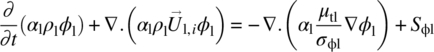
For most of the operating regimes used in practice, flows in multiphase stirred vessels are turbulent. Therefore, the mass and momentum balance equations governing such flows can be written as (Favre averaged equations for each phase without considering mass transfer)

where
-
 is the turbulent dispersion force accounting for the turbulent fluctuation in the phase volume fraction.
It is modeled as

Here, Vdr is the drift velocity, Dp and Dq are the diffusivities of the continuous and dispersed phase, respectively, and σpq is the turbulent Prandtl number. The diffusivities Dp and Dq can be calculated from the turbulent quantities following the work of Simonin and Viollet [10]. The turbulent Prandtl number σpq is usually set to 0.75–1.0. ![]() is the stress tensor in the phase q due to molecular viscosity, and
is the stress tensor in the phase q due to molecular viscosity, and ![]() is the Reynolds stress tensor of phase q (representing contributions of correlation of fluctuating velocities in momentum transfer). Boussinesq's eddy viscosity hypothesis is usually used to relate the Reynolds stresses with gradients of time‐averaged velocity as
is the Reynolds stress tensor of phase q (representing contributions of correlation of fluctuating velocities in momentum transfer). Boussinesq's eddy viscosity hypothesis is usually used to relate the Reynolds stresses with gradients of time‐averaged velocity as

Here, μtq is the turbulent viscosity of the phase q and I is the unit tensor.
The turbulent viscosity may be related to the characteristic velocity and length scales of turbulence. Several turbulence models have been proposed to devise suitable methods/equations to estimate these characteristic length and velocity scales in order to close the set of equations. Despite the known deficiencies, the overall performance of the standard k–ε turbulence model for simulating flows in stirred vessels is adequate for many engineering applications [9]. Most of the modeling attempts of complex turbulent multiphase flows mainly rely on the practices followed for the single‐phase flows, with some ad hoc modifications to account for the presence of dispersed phase particles. Here we present the standard k–ε turbulence model to estimate the turbulent viscosity of the liquid phase without going into critical review of different models and approaches. Additional details may be found in Ranade [9]. The governing equations for turbulent kinetic energy, k, and turbulent energy dissipation rate, ε, are listed below:
where
- ϕl is the turbulent kinetic energy or turbulent energy dissipation rate in the liquid phase.
The symbol σϕl denotes the turbulent Prandtl number for variable ϕ. Sϕl is the corresponding source term for ϕ in liquid phase. Note that the turbulence equations are solved only for the continuous liquid phase. Source terms for turbulent kinetic energy and dissipation can be written as

where
- Gl is generation in the liquid phase.
- Gel is extra generation (or dissipation) of turbulence in the liquid phase.
Generation due to mean velocity gradients, Gl and μtl, turbulent viscosity was calculated as
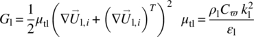
Extra generation or damping of turbulence due to the presence of dispersed phase particles is represented by Gel. Kataoka et al. [11] have analyzed the influence of the gas bubbles on liquid‐phase turbulence. Motion of larger bubbles generates extra turbulence. However, their analysis indicates that the extra dissipation due to small‐scale interfacial structures almost compensates for the extra generation of turbulence due to large bubbles. Numerical experiments on bubble columns also indicate that one may neglect the contribution of extra turbulence generation (see Ref. [12] for more details). Therefore, for stirred vessels where impeller rotation generates significantly higher turbulence than that observed in bubble columns, the contribution of the additional turbulence generation due to bubbles can be neglected.
Following the general practice, the same values of parameters proposed for single‐phase flow (C1ε = 1.44, C2ε = 1.92, C3ε = 1.3, Cμ = 0.09, σk = 1.0, and σε = 1.3) may be used to simulate the turbulence in two‐phase flow. In the dispersed k–ε turbulence model, no extra transport equations were solved for estimating the turbulent quantities for dispersed phase. Instead, a set of algebraic relations can be used to couple the dispersed phase turbulence to continuous phase turbulence using Tchen's theory [10, 13]. The turbulence of dispersed phase depends mainly on three important time scales, characteristic time of turbulent eddy ![]() , bubble relaxation time
, bubble relaxation time ![]() , and eddy–bubble interaction time
, and eddy–bubble interaction time ![]() (see Ref. [14] for more details). This approach of modeling turbulent dispersed phase is computationally less expensive and can adequately simulate the turbulence in two‐phase flow with low dispersed phase holdup (<10%). In the case of higher dispersed phase holdup, simulating turbulence equations for individual phases may be required.
(see Ref. [14] for more details). This approach of modeling turbulent dispersed phase is computationally less expensive and can adequately simulate the turbulence in two‐phase flow with low dispersed phase holdup (<10%). In the case of higher dispersed phase holdup, simulating turbulence equations for individual phases may be required.
Interphase coupling terms make multiphase flows fundamentally different from single‐phase flows. The formulation of time‐averaged ![]() , therefore, must proceed carefully. The interphase momentum exchange term consists of four different interphase forces: Basset history force, lift force, virtual mass force, and drag force [15]. Basset force arises due to the development of a boundary layer around bubbles and is relevant only for unsteady flows. The Basset force involves a history integral, which is time consuming to evaluate, and in most cases, its magnitude is much smaller than the interphase drag force. Considering this, the Basset history force is usually not considered for simulating dispersed multiphase flows in stirred vessels. The interphase momentum exchange term that included the lift, virtual mass, and drag force terms is written as
, therefore, must proceed carefully. The interphase momentum exchange term consists of four different interphase forces: Basset history force, lift force, virtual mass force, and drag force [15]. Basset force arises due to the development of a boundary layer around bubbles and is relevant only for unsteady flows. The Basset force involves a history integral, which is time consuming to evaluate, and in most cases, its magnitude is much smaller than the interphase drag force. Considering this, the Basset history force is usually not considered for simulating dispersed multiphase flows in stirred vessels. The interphase momentum exchange term that included the lift, virtual mass, and drag force terms is written as
The virtual mass term in i direction is given as

where
- CVM is virtual mass coefficient.
In the present work, the value of CVM was set to 0.5.
The lift force in i direction is given as
The interphase drag force exerted on phase 2 in i direction is given by

where
- CD is a drag coefficient.
This expression can be generalized to more than one dispersed phases in a straightforward way. It is necessary to correct the estimation of drag coefficient to account for the particle size distribution and nonspherical shapes of the particles, for the presence of other particles, and for the presence of prevailing turbulence. Specific discussion of these as well as formulation of boundary conditions related to simulations of multiphase flows in stirred vessels is included in the following sections.
Denser suspensions of gas or liquid phases within continuous liquid phase lead to issues like coalescence and breakup. It is possible to extend the approach to incorporate population balance models to account for such processes. However, this may require significantly larger computational resources as well as input data on model parameters of coalescence and breakup kernels. Presence of dense solid suspension exhibits various additional complexities and requires substantial modifications in the governing equations. The governing equations for such cases are not included here for the sake of brevity and may be found in Ranade [9]. Other conservation equations (enthalpy and species) for multiphase flows that can be written following the similar general format are also not included here. Application of these governing equations to simulate multiphase flows in stirred vessels is discussed in the following.
13.2.2 Application to Simulate Gas–Liquid Flow in Stirred Reactor
The most important step in the application of model equations to simulate a gas–liquid stirred reactor is the appropriate selection of interphase force formulations. They play a very important role while simulating gas dispersion [16]. Lane et al. [16] carried out order‐of‐magnitude analysis of all interphase forces. They observed that in the bulk region of the stirred reactor, interphase drag force dominates the total magnitude of interphase forces and hence can determine the gas dispersion pattern. There are few studies available in the literature highlighting the influence of interphase drag force on the predicted gas holdup distribution (for example, Refs. [17, 18]). However, not much information is available in the literature on the virtual mass force and lift force and their effect on the predicted gas holdup distribution. To explain the influence of different interphase forces, we reproduce some of the results obtained by Khopkar and Ranade [17]. They have carried out simulations of gas–liquid flow in a stirred vessel in an experimental setup used by Bombac et al. [19]. All the relevant dimensions like impeller diameter, impeller off‐bottom clearance, reactor height and diameter, sparger location and diameter, and so on were the same as used by Bombac et al. [19]. Considering the symmetry of the geometry, half of the reactor was considered as a solution domain (see Figure 13.1). The solution domain and details of the finite volume grid used were similar to those used by Khopkar and Ranade [17]. A QUICK discretization scheme with SUPERBEE limiter function (to avoid nonphysical oscillations) was used. Standard wall functions were used to specify wall boundary conditions. The computational results are discussed in the following section.

FIGURE 13.1 Computational grid and solution domain of stirred reactor.
Source: Reprinted with permission from Khopkar and Ranade [7], Copyright 2011 John Wiley and Sons Inc.
13.2.2.1 Interphase Forces
13.2.2.1.1 Interphase Drag Force
In stirred reactors, bubbles experience significantly higher turbulence generated by impellers. Unless the influence of this prevailing turbulence on bubble drag coefficient is accounted, the CFD model was not found to predict the pattern of gas holdup distribution adequately. Relatively few attempts (experimental as well as numerical) have been made to understand the influence of prevailing turbulence on drag coefficient (see, for example, Refs. [18, 20–23]). Bakker and van den Akker [20], Brucato et al. [21], and Lane et al. [18] have attempted to relate the influence of turbulence on drag coefficient to the characteristic spatiotemporal scales of prevailing turbulence and therefore seem to be promising. Khopkar and Ranade [17] evaluated the three alternative proposals using a two‐dimensional (2D) CFD‐based model problem. They have observed that the predicted results deviate from the trends estimated by correlation of Lane et al. [18]. However, the predicted results show reasonable agreement with estimation based on correlation Bakker and van den Akker [20] (Eq. 13.12) and Brucato et al. [21] (Eq. 13.13), with 100 times lower correlation constant (K = 6.5 × 10⁻⁶). Interestingly, in both of these correlations, they have used volume‐averaged values of the turbulent viscosity and Kolmogorov scale, respectively:


where
- CD is the drag coefficient in turbulent liquid.
- CD0 is the drag coefficient in a stagnant liquid.
- db is bubble/particle diameter.
- λ is the Kolmogorov length scale (based on volume‐averaged energy dissipation rate).
The gas–liquid flow in stirred reactor was simulated using the drag coefficients estimated with volume average values of Kolmogorov scale (Eq. 13.13) and turbulent viscosity (Eq. 13.12) for operating conditions of Fl = 0.1114 and Fr = 0.3005. This operating condition represents L33 flow regime (large 33 cavities) in stirred reactor. The quantitative comparison of the predicted gas holdup distribution with the experimental data [19] is shown in Figure 13.2. It can be seen from Figure 13.2a and b that the gas holdup distribution predicted based on Eq. (13.12) shows fairly different gas distribution from the experimental data (shown in Figure 13.2a). The major disagreement was observed in the region below the impeller. The impeller‐generated flow was not sufficient to circulate gas in a lower circulation loop. The computational model has underpredicted total gas holdup (predicted holdup was 2.55% compared to the experimental measurement of 3.3%). The predicted results based on Eq. (13.13) are closer to the experimental data (see Figure 13.2a and c). This model resulted in overprediction of total gas holdup (predicted holdup was 3.97% compared to the experimental measurement of 3.3%). Despite the overprediction, the predicted gas holdup distribution showed better agreement with the data than predicted by Eq. (13.12). Equation (13.13) can therefore be recommended for carrying out gas–liquid flow simulations in stirred tanks.

FIGURE 13.2 Comparison of experimental and predicted gas holdup distribution at mid‐baffle plane for L33 flow regime, Fl = 0.1114 and Fr = 0.3005. (a) Experimental [19]. (b) Predicted results with Bakker and van den Akker correlation (Eq. 13.12). (c) Predicted results with modified Brucato et al. correlation, (Eq. 13.13). (Contour labels denote the actual values of gas holdup in percentage).
Source: Reprinted with permission from Khopkar and Ranade [17]. Copyright 2006 American Institute of Chemical Engineers.
13.2.2.1.2 Virtual Mass and Lift Force
The other two important interphase forces are virtual mass force and lift force. The virtual mass effect is significant when the secondary phase density is much smaller than the primary phase density. The effect of the virtual mass force was first studied. The predicted gas holdup distributions obtained with and without considering virtual mass force are shown in Figure 13.3a and b. It can be seen from Figure 13.3 that the influence of the virtual mass force on the predicted pattern of gas distribution was significant only in the impeller discharge stream. However, the influence of virtual mass force was not found to be significant in the bulk of the reactor. It should be noted that the value of virtual mass coefficient used in the present study (0.5) is valid for spherical bubble and may not be appropriate for wobbling bubbles. The reported value of virtual mass coefficient is somewhat higher than 0.5 (see, for example, Ref. [24]). However, it should be noted that the predicted results are not very sensitive to the consideration of virtual mass terms. A comparison of the predicted results obtained with values of virtual mass coefficients as 0 and 0.5 did not show any significant differences (see Figure 13.3). Considering this, no specific effort was made to obtain accurate value of virtual mass coefficient.

FIGURE 13.3 Comparison of predicted gas holdup profiles for with and without virtual mass and lift force effect for L33 flow regime, Fl = 0.1114 and Fr = 0.3005. (a) Predicted, without virtual mass and lift force effect: mid‐baffle plane. (b) Predicted, with virtual mass effect: mid‐baffle plane. (c) Predicted, with lift force effect: mid‐baffle plane. (Contour labels denote the actual values of gas holdup in percentage).
Source: Reprinted with permission from Khopkar and Ranade [17]. Copyright 2006 American Institute of Chemical Engineers.
Similarly, the simulations were carried out with and without considering lift force. The predicted gas holdup distribution obtained with considering lift force is shown in Figure 13.3c. It can be seen from Figure 13.3 that the influence of lift force on the predicted pattern of gas distribution was significant in the impeller discharge stream and below impeller region. The predicted results with lift force predict a lower gas holdup in the region below impeller. In the upper impeller region of the reactor, the influence of lift force was not found to be significant. Therefore, it can be said that the modeling of lift force and virtual mass force may not be essential while simulating gas–liquid flow in stirred vessels.
13.2.2.2 Modeling Bubble Size Distribution
In a gas–liquid stirred reactor, gas bubbles of different sizes coexist. Very fine bubbles are observed in the impeller discharge stream (<1 mm), whereas bubbles of the size of few mm (~5 mm) are observed in the region away from the impeller [25]. The width of the bubble size distribution (BSD) depends upon the turbulence level and prevailing flow regime. Appropriate selection of bubble sizes is very important for the correct prediction of the slip velocity and mass transfer area. Both the slip velocity and mass transfer area can be more accurately estimated by modeling with local BSDs. Local bubble size or gas–liquid mass transfer can be estimated more accurately from local BSDs based on either a population balance [26] or by modeling the bubble number density function [18]. The bubble density function approach [18] is computationally less intensive and requires one additional equation to solve along with the two‐fluid model. This approach predicts the Sauter mean diameter at every grid node point. The predicted results of Lane et al. [18] show reasonable agreement with the experimental data of Barigou and Greaves [25]. Laakkonen et al. [26] simulated the gas–liquid flows in a stirred reactor using population balance modeling. Their simulated results are discussed here to explain the need for modeling the BSD while simulating gas–liquid flow in stirred reactors. The details of the population balance formulation, bubble breakage, and coalescence model are not discussed here and can be found in Laakkonen et al. [26]. The influence of the prevailing turbulence on the interphase drag force was modeled with a slightly modified Bakker and van den Akker [20] correlation. The comparison of the predicted BSD and the mean bubble diameter with the experimental data is shown in Figure 13.4. The following conclusions can be drawn from the comparison between predicted results and experimental data:
- The parameters of the coalescence and breakage models were tuned to fit the experimental measurements. This limits the applicability of the model for different configurations of stirred reactor.
- The tails in the predicted volume BSDs are larger compared to the experimental measurements indicating underprediction of breakage process. The rate of breakage process is dependent on the predicted values of the turbulent energy dissipation rate. The CFD model underpredicts the turbulent kinetic energy dissipation rates and hence led to lower rate of bubble breakage process.
- The enormous requirement of computational requirement for multi‐fluid model does not allow modeler to use fine mesh for simulating the turbulent multiphase flow. The use of a relatively coarse mesh significantly contributes to the underprediction of turbulent properties and hence influences the predicted breakage and coalescence rates.

FIGURE 13.4 Comparison of predicted bubble size distribution with experimental data. (a) Local bubble size distributions in the air–water dispersion, 14 L tank, N = 700 rpm, and Q = 0.7 vvm. (b) Mean diameters (mm).
Source: Reprinted with permission from Laakkonen et al. [26]. Copyright 2006 Elsevier Ltd.
The present state of understanding of the breakage and coalescence processes and the unavailability of experimental data for different reactor configurations suggest that it may not be advantageous to use population balance‐based multi‐fluid models while simulating industrial gas–liquid stirred reactors. It may be more effective to use effective combination of bubble diameter and interphase drag coefficient to get realistic results.
13.2.2.3 Gas Holdup Distribution in L33, S33, and VC Flow Regimes
Gas–liquid flows generated by the Rushton turbine in a stirred vessel were simulated for other two flow regimes representing S33 (Fl = 0.0788; Fr = 0.6) and VC (Fl = 0.026 267; Fr = 0.6). As discussed previously, Eq. (13.13), based on volume‐averaged dissipation rate and Kolmogorov scale (λ), was used to calculate effective drag coefficients. Comparisons of predicted gas holdup distributions with the experimental results at the mid‐baffle plane are shown in Figure 13.5. It can be seen from these figures that the predicted gas holdup distributions for S33 and VC flow regimes are in reasonably good agreement with the experimental data. However, the computational model overpredicted the values of total gas holdup. The predicted value of total gas holdup (4.85%) was higher than the reported experimental value (4.2%) for the S33 flow regime. Similarly, the predicted value of total gas holdup (2.63%) was higher than the experimental data (2.2%) for the VC flow regime.
FIGURE 13.5 Comparison of experimental and predicted gas holdup distribution for S33 and VC flow regimes (experimental data of Bombac et al. [19]). (a) Experimental, S33 flow regime, Fl = 0.0788 and Fr = 0.3005 (mid‐baffle). (b) Predicted, S33 flow regime, Fl = 0.0788 and Fr = 0.6 (mid‐baffle). (c) Experimental, VC flow regime, Fl = 0.026 267 and Fr = 0.6 (mid‐baffle). (d) Predicted, VC flow regime, Fl = 0.026 267 and Fr = 0.6 (mid‐baffle). (Contour labels denote the actual values of gas holdup in percentage).
Source: Reprinted with permission from Khopkar and Ranade [17]. Copyright 2006 American Institute of Chemical Engineers.
Comparisons of axial profiles of radially averaged gas holdup for all three regimes are shown in Figure 13.6. It can be seen from Figure 13.6 that the computational model overpredicts the values of gas holdup in the region above the impeller for all three regimes. The maximum value of predicted radially averaged gas holdup occurs at an axial distance of 0.117 m for L33 and 0.107 m for S33 as well as VC regimes compared with the experimentally observed distance of 0.13 m for L33 and 0.1125 m for S33 as well as VC regimes. The predicted values of gas holdups at this maximum are underpredicted (7.3% for L33, 7.94% for S33, and 3.82 for VC) compared with the experimental value (8.1% for L33, 8.8% for S33, and 4.1% for VC). Quantitative comparisons of angle‐averaged values of predicted gas holdup and experimental data at three different axial locations for all three regimes are shown in Figure 13.7. It can be seen from Figure 13.7 that comparisons of the predicted values of gas holdup and experimental data are reasonably good for all three regimes. The computational model was thus able to simulate all three regimes reasonably well.
FIGURE 13.6 Comparison of predicted axial profile of radially averaged gas holdup with experimental data for L33, S33, and VC flow regimes (symbol denotes the experimental data of Bombac et al. [19]).
Source: Reprinted with permission from Khopkar and Ranade [17]. Copyright 2006 American Institute of Chemical Engineers.

FIGURE 13.7 Comparison of predicted angle‐averaged values of gas holdup (α2) with experimental data for L33, S33, and VC flow regimes. (a) L33 flow regime, Fl = 0.1114 and Fr = 0.3005. (b) S33 flow regime, Fl = 0.0788 and Fr = 0.6. (c) VC flow regime, Fl = 0.026267 and Fr = 0.6. ● Experimental data [19]; — Predicted results.
Source: Reprinted with permission from Khopkar and Ranade [17]. Copyright 2006 American Institute of Chemical Engineers.
13.2.2.4 Gross Characteristics
Predicted influence of the gas flow rate on gross characteristics, power, and pumping numbers is also of interest. Pumping and power numbers were calculated from simulated results as


where
- B is blade height.
- Di is impeller diameter.
- N is impeller speed.
- ri is impeller radius.
- Ur is radial velocity.
The calculated values of pumping and power number from the simulated results are listed in Table 13.3. As the gas flow rate increases, impeller pumping as well as power dissipation decreases. The extent of decrease increases with an increase in the gas flow rate (or in other words, as flow regime changes from VC to S33 and further to L33). Bombac et al. [19] have not reported their experimental values of power dissipation or pumping number. In the absence of such data, the predicted values were compared with the estimates of empirical correlations proposed by Calderbank [27], Hughmark [28], and Cui et al. [29]. While demonstrating the qualitative trend, the CFD model underpredicts the decrease in power dissipation in the presence of gas compared to the estimates of these correlations. CFD model, however, could correctly capture the overall gas holdup distribution and can therefore simulate different flow regimes of gas–liquid flow in stirred reactors.
13.2.3 Application to Simulate Solid–Liquid Flow in Stirred Reactor
Suspension of solid particles in a stirred reactor either in presence or in absence of gas is commonly encountered in chemical process industry (refer to Table 13.1). All these processes involve mass transfer between the solid and liquid phases. There are various studies reported in literature, such as Nienow [30], Nienow and Miles [31], Chaudhari [32], and Conti and Sicardi [33], explaining the effect of agitation on the mass transfer coefficient, kSL. They observed that the agitation speed influences the mass transfer coefficient (see Figure 13.8). This phenomenon was explained through the two important parameters, viz. mesoscopic availability of solids in bulk vessel volume or suspension quality and the rate of renewal of the diffusional boundary layer around the solid particle. The mass transfer curve clearly explains that before complete suspension, the mass transfer coefficient linearly increases with the impeller speed and after that the rate of increase drops. This suggests that before complete suspension, both the parameters positively increase with an increase in the impeller rotational speed. However, the mesoscopic availability of solids in bulk vessel volume does not change much after complete suspension condition, and hence the rate of increase in mass transfer rate with an increase in impeller rotational speed drops after the complete suspension condition. Additional energy dissipation does not yield much benefit in mass transfer after it.

FIGURE 13.8 Influence of suspension quality on the mass transfer coefficient.
Source: Reprinted with permission from Atiemo‐Obeng et al. [34]. Copyright 2004 John Wiley and Sons Inc.
Despite significant research efforts, prediction of design parameters to ensure an adequate solid suspension is still an open problem for design engineers. Design of stirred slurry reactors relies on empirical correlations obtained from the experimental data. These correlations are prone to great uncertainty as one departs from the limited database that supports them. Moreover, for higher values of solid concentration, very few experimental data on local solid concentration is available because of the difficulties in the measurement techniques. Considering this, it would be most useful to develop computational models, which will allow “a priori” estimation of the solid concentration over the reactor volume.
The discussed two‐fluid model is applied to simulate solid–liquid flow in a stirred reactor. In addition to interphase drag force, turbulent dispersion force plays an important role while simulating solid–liquid flows. There are few studies available in the literature highlighting the influence of interphase drag force on the predicted solid holdup distribution (for example, Refs. [35–37]). To explain the influence of different interphase forces, we reproduce some of the results obtained by Khopkar et al. [37]. They have carried out simulations of solid–liquid flow in a stirred vessel in an experimental setup used by Yamazaki et al. [38]. The system investigated consists of a cylindrical flat‐bottomed reactor (of diameter, T = 0.3 m; liquid height, H = T). Four baffles of width 0.1T were mounted perpendicular to the reactor wall. The shaft of the impeller was concentric with the axis of the reactor. A standard Rushton turbine with diameter D = T/3 has been used. The impeller off‐bottom clearance has been set equal to C = T/3, measured from the bottom of the reactor to the center of the impeller blade height. Water as liquid phase and glass beads (having density equal to 2470 kg/m3 and particle diameter, dp = 264 μm) as solid phase were used in the simulations.
Considering geometrical symmetry, half of the reactor was considered as a solution domain. It is very important to use an adequate number of computational cells while numerically solving the governing equations over the solution domain. The prediction of the turbulence quantities is especially sensitive to the number of grid nodes and grid distribution within the solution domain. In the present work, the numerical simulations for solid–liquid flows in stirred reactor have been carried out with grid size of 298 905 (r × θ × z: 57 × 93 × 57). The details of computational grid used in the present work are shown in Figure 13.9. In the present work, the standard wall functions were used to specify wall boundary conditions.

FIGURE 13.9 Computational grid and solution domain of stirred reactor.
Source: Reprinted with permission from Khopkar et al. [37]. Copyright 2006 American Chemical Society.
13.2.3.1 Interphase Drag Force
In stirred reactors, particles experience significantly higher turbulence generated by impellers. Similar to the discussion included in previous subsection, unless the influence of this prevailing turbulence on particle drag coefficient is accounted, the CFD model will not predict the solid suspension adequately. Khopkar et al. [37] evaluated the two alternative proposals [21, 39] using a 2D CFD‐based model problem. They have observed that the predicted results deviate from the trends estimated by correlation of Pinelli et al. [39]. However, the predicted results show reasonable agreement with estimation based on correlation by Brucato et al. [21]. They correlated the predicted results by considering the sole dependence on dp/λ for a range of solid holdup values (5 < α < 25%). They observed that the predicted results require ten times lower proportionality constant (K = 8.76 × 10⁻⁵) in Eq. (13.13) as compared with that proposed by Brucato et al. [21].
Solid–liquid flow generated by the Rushton turbine has been simulated for a solid volume fraction equal to 10.0%, dp = 264 μm, and at an impeller rotation speed N = 20 rps. Both the formulation of drag coefficient and actual Brucato et al. [21] (K = 8.76 × 10⁻⁴) and the modified Brucato correlation (K = 8.76 × 10⁻⁵) were used for the evaluation of the interphase drag force formulation. The value of dispersion Prandtl number, σpq, has been set to the default value of 0.75. The predicted solid holdup distributions by using both drag coefficient formulation at the mid‐baffle plane are shown in Figure 13.10a and b. It can be seen from Figure 13.10a that with actual Brucato et al. [21] correlation, the computational model has predicted almost complete suspension of the solid particles. However, the simulated solid holdup distribution using modified Brucato et al. [21] did not capture the complete suspension of solid particles in stirred reactor (see Figure 13.10b). The simulated solid holdup distribution shows the presence of solid accumulation at the bottom and near the axis of the reactor. For quantitative comparison the predicted solid concentrations/holdups were compared with the experimental data of Yamazaki et al. [38]. The quantitative comparison of the azimuthally averaged axial profile of solid holdup at a radial location (r/T = 0.35) is shown in Figure 13.10c. It can be seen from Figure 13.10c that the computational model with drag coefficient formulation of Brucato et al. [21] has overpredicted the solid suspension height. However, the suspension height predicted by the modified Brucato correlation is in good agreement with the experimental data. It can also be seen from Figure 13.10 that solid holdup distribution predicted with the use of modified Brucato et al. [21] correlation has captured the presence of higher solid concentration in the impeller discharge stream (a bell shaped in the concentration profile), which is a characteristic of the solid–liquid flow generated by Rushton turbine. However the prediction with Brucato et al. [21] correlation does not show any such characteristics. Overall, it can be said that the modified Brucato et al. [21] correlation predicted solid holdup distribution in stirred vessel more accurately.

FIGURE 13.10 Simulated solid holdup distribution at mid‐baffle plane, for dp = 264 μm, dp/λ ≈ 20, α = 0.1, N = 20.0 rps, and Utip = 6.283 m/s. (a) K = 8.76 × 10⁻⁴. (b) K = 8.76 × 10⁻⁵. (c) Comparison of predicted results with experimental data.
Source: Reprinted with permission from Khopkar et al. [37]. Copyright 2006 American Chemical Society.
13.2.3.2 Turbulent Dispersion Force
The developed computational model was then extended to study the influence of the turbulent dispersion force on the suspension quality in the stirred reactor. The magnitude of the turbulent dispersion force was varied by varying the value of the dispersion Prandtl number, σpq, in the range of 0.0375–3.75. Figure 13.11 shows the comparison of the predicted solid concentration distribution in the stirred reactor with the experimental data of Yamazaki et al. [38] with and without turbulent dispersion force. It can be seen from Figure 13.11 that the turbulent dispersion has a significant effect on the predicted suspension quality in the stirred reactor. The computational model predicted a more uniform suspension with a decrease in the value of dispersion Prandtl number. This is expected as the drift velocity (or turbulent dispersion force) is inversely proportional to the dispersion Prandtl number (see Eq. (13.3)). Decreasing the latter means increase in the turbulent dispersion force, which consequently results in more dispersion of the particles, resulting in more uniform suspension. Overall, it can be said that the simulations carried out with σpq = 0.375 and 0.0375 have overpredicted the suspension quality. However, for σpq = 3.75 the computational model has underpredicted the suspension quality. Therefore, CFD simulation of solid–liquid stirred reactor needs to be carried out with σpq = 0.75 for adequate prediction of suspension quality.

FIGURE 13.11 Effect of turbulent dispersion force on the predicted solid concentration, for dp = 264 μm, dp/λ ≈ 20, α = 0.1, N = 20 rps, and Utip = 6.283 m/s.
Source: Reprinted with permission from Khopkar and Ranade [7]. Copyright 2011 John Wiley and Sons Inc.
13.2.4 Application to Simulate Gas–Solid–Liquid Flow in Stirred Reactor
Suspension of solid particles in the presence of gas has various applications in the process industry. These applications include catalytic hydrogenations, oxidations, fermentations, evaporative crystallizations, and froth flotation. In a gas–liquid–solid system, the impeller plays a dual role of keeping the solids suspended in the liquid while dispersing the gas bubbles. Dyalag and Talaga [40] have found that in a gas–liquid–solid stirred reactor, the gas phase is always uniformly dispersed before the solids are completely suspended. Therefore, the formation of a completely dispersed three‐phase system depends on the condition under which the solids are suspended by the impeller action. Identification of these operating conditions is very important for operating a stirred reactor in an energy‐efficient mode. Some mass transfer studies (for example, Ref. [31]) in two‐phase solid–liquid mixing in stirred tanks have also shown that the particle–fluid mass transfer rate is comparable at the just off‐bottom suspension (JS) point, irrespective of the power input level. Any incremental power input beyond this point for improving the mass transfer coefficient is often uneconomical. Attempts to extend the above hypothesis to three‐phase systems introduce an additional complexity, as the impeller pumping efficiency changes in the presence of gas. It is also observed that the tank, impeller, and sparger geometry variations that have been proposed [41–43] are highly system specific with respect to gas–liquid and solid–liquid systems and may not be possible to directly extend to gas–liquid–solid systems. It is therefore necessary to develop tools to examine the role of reactor hardware in meeting the demands associated with the simultaneous gas dispersion and solid suspension.
Critical analysis of available literature suggests that practically no information is available in the literature on the CFD simulation of three‐phase gas–liquid–solid stirred reactor. Complex interactions between the solid particles, gas bubbles, and the liquid phase make the fluid dynamics of three‐phase stirred reactor very complex. Recently, Murthy et al. [44] made an attempt to simulate a three‐phase stirred reactor. They used the approach proposed by Khopkar and Ranade [17] for modeling gas–liquid flow and approach of Pinelli et al. [39] for simulating solid–liquid flow. Murthy et al. [44] were able to predict the critical impeller speed required for solid suspension. However, their study was limited to very low solids loading (maximum solids loading is <10 wt %). The applicability of the same computational model to simulate solid suspension at higher solids loading (>20 wt % or 10% by volume fraction) is not known. In this work, a CFD model was developed to simulate solid suspension in a three‐phase stirred reactor. The approaches discussed in the last two subsections were used to model the gas–liquid and solid–liquid interactions in the three‐phase stirred reactor.
Experimental setup of Pantula and Ahmed [45] was used to simulate gas–liquid–solid flows in a stirred reactor. The system investigated consists of a cylindrical flat‐bottomed reactor (of diameter, T = 0.4 m; liquid height, H = T). Four baffles of width 0.1T were mounted perpendicular to the reactor wall. The shaft of the impeller was concentric with the axis of the reactor. A standard Rushton turbine with diameter D = T/3 has been used. The impeller off‐bottom clearance has been set equal to C = T/4, measured from the bottom of the reactor to the center of the impeller blade height. A ring sparger of diameter Ds = 2D/3 with evenly spaced holes at a clearance (Cs) of T/6 was provided for gas input. Water as liquid phase, air as gas phase, and glass beads (having density equal to 2500 kg/m3 and particle diameter dp = 174 μm) as solid phase were used in the simulations. Simulations were carried out with solid‐phase volume fraction equal to 12% (i.e. 30 wt %).
Considering the geometrical symmetry, half of the reactor was considered as a solution domain. In the present work, the numerical simulations for gas–liquid–solid flows in stirred reactor have been carried out with grid size of 436 170 (r × θ × z: 70 × 93 × 67). The details of computational grid used in the present work are shown in Figure 13.12. In the present work, the standard wall functions were used to specify wall boundary conditions.

FIGURE 13.12 Computational grid and solution domain of stirred reactor.
Source: Reprinted with permission from Khopkar and Ranade [7]. Copyright 2011 John Wiley and Sons Inc.
13.2.4.1 Solid Suspension in an Aerated Stirred Vessel
Minimum speed for JS is a very important hydrodynamic parameter for designing gas–liquid–solid stirred reactor. Experimental studies so far on gas–liquid–solid suspensions have clearly indicated the requirement of increased suspension speed, thereby more power input, on the introduction of gas [40–43]. This is because of a decrease in impeller pumping efficiency and power draw due to the formation of ventilated cavities behind the impeller blades on gassing [46]. Recently, Zhu and Wu [47] carried out experimental measurements in a three‐phase stirred reactor to determine the JS speed for a variety of solid sizes, solids loading, impeller sizes, and tank sizes. They suggested the possibility of relating relative just off‐bottom suspension speed (RJSS) with just suspension aeration number (based on just suspension speed for solid–liquid system). They also observed that the proposed relation was independent of impeller size, solid size, solids loading, and tank size and can be used to scale up laboratory data to full‐scale vessel. The same definition (Eq. 13.16) was used in the present study to identify the JS speed for different gas flow rates:

where
- m and n are constants.
For the Rushton turbine, the values of m and n are 2.6 and 0.7, respectively. The simulations were carried out for three just suspension aeration numbers: 0, 0.025, and 0.05. The impeller rotational speeds (Njsg) for the three aeration numbers are 9.30, 11.16, and 12.27 rps, respectively.
The predicted solid holdup distribution at mid‐baffle plane for all three aeration numbers is shown in Figure 13.13. It can be seen from Figure 13.13 that for three‐phase system the computational model has predicted more accumulation of solids at the bottom of reactor near the central axis in comparison with the two‐phase system. The predicted cloud height values were also found to drop in the presence of gas. The predicted solid volume fraction values were then used to describe the suspension quality in the reactor. The criterion based on the standard deviation value, calculated using Eq. (13.17), was used to describe suspension quality for all three cases. It was observed that the computational model predicted standard deviation value (σ) equal to 0.45 for two‐phase flow. However, for three‐phase flow, computational model predicted σ equal to 0.82 and 0.90 for Najs equal to 0.025 and 0.05, respectively. Overall, it can be said that the computational model has predicted JS condition for two‐phase flow (σ < 0.8), but incomplete suspension for three‐phase system (σ > 0.8):


FIGURE 13.13 Simulated solid holdup distribution at mid‐baffle plane, for dp = 174 μm and αs = 0.12. (a) Najs = 0 and N = 9.3 rps. (b) Najs = 0.025 and N = 11.16 rps. (c) Najs = 0.05 and N = 12.27 rps.
Source: Reprinted with permission from Khopkar and Ranade [7]. Copyright 2011 John Wiley and Sons Inc.
The predicted gas holdup distribution at mid‐baffle plane for two suspension aeration numbers is shown in Figure 13.14. It can be seen from Figure 13.14 that for both conditions, the computational model has predicted higher values of gas holdup in both circulation loops of flow. This indicates that the computational model predicted complete dispersion condition of gas phase in the vessel. These predicted results also support the experimental observations made by Dyalag and Talaga [40] on quality of gas dispersion.

FIGURE 13.14 Simulated gas holdup distribution at mid‐baffle plane, for dp = 174 μm and αs = 0.12. (a) Najs = 0.025. (b) Najs = 0.05.
Source: Reprinted with permission from Khopkar and Ranade [7]. Copyright 2011 John Wiley and Sons Inc.
13.2.4.2 Gross Characteristics
Predicted influence of the gas flow rate on gross characteristics, power number, gas holdup, and suspension quality is also of interest. The calculated values of power number, gas holdup, and standard deviation from the simulated results are listed in Table 13.4. Few conclusions can be drawn from Table 13.4. First, the computational model has predicted the drop in impeller power number value in the presence of gas. While demonstrating the qualitative trend, the CFD model has underpredicted the actual power number value (predicted value of power number for single‐phase flow equal to 3.85). Second, the CFD model was able to predict just suspension condition for solid–liquid flows. However, the model failed to predict just suspension condition in the presence of gas. The standard deviation value (describing suspension quality) increases with an increase in gas flow rate. For lower aeration rate the model has predicted the total gas holdup values reasonably well. However, model has underpredicted total gas holdup value for higher aeration rate. Overall, CFD model with the presented modeling approach could reasonably predict gas–liquid–solid flow in a stirred reactor at low aeration rates. Further work is needed to develop adequately accurate model capable of simulating gas–liquid–solid flow in stirred reactor at higher aeration rates.
TABLE 13.4 Gross Characteristics of a Gas–Liquid–Solid Stirred Reactor
Source: Reprinted with permission from Khopkar and Ranade [7]. Copyright 2011 John Wiley and Sons Inc.
| Just Suspension Aeration Number, Najs | Predicted Total Gas Holdup (%), εg | Estimated Gas Holdup (%), [45] | Standard Deviation, σ | Predicted Power Number, NP |
| 0 | — | — | 0.45 | 3.95 |
| 0.025 | 5.33 | 4.80 | 0.81 | 2.61 |
| 0.05 | 6.45 | 9.55 | 0.90 | 2.54 |
13.2.5 Application to Simulate Liquid–Liquid Flows in Stirred Reactor
Stirred tanks represent the most popular reactors and mixers that are widely used in carrying out operations involving liquid–liquid dispersions. Drop size distributions and dynamics of their evolution are important characteristics of such dispersions as they are related to the rate of mass transfer and chemical reactions that may occur in a process. In some cases the drops are stabilized against coalescence by the addition of stabilizers to have drops sized by agitation before chemical reaction begins (suspension polymerization). In other areas the breakup and coalescence processes can affect directly a reaction in the dispersed phase. It is well known that other than physical chemistry, fluid dynamic interaction between the two phases plays a significant role in determining the features of the dispersion, but it is far from being fully understood. Average properties over the whole vessel are usually considered for system description and for scale‐up. The following main aspects have been studied: minimum agitation speed for complete liquid–liquid dispersion [48], correlation of mean drop size and DSD to energy dissipation rate and mixer geometric parameters [49] as well as to energy dissipation rate and flow in the vessel [50], the influence of various impellers on the dispersion features [50–52], and description of the interaction between the liquid phases in terms of intermittent turbulence [53–56].
CFD modeling of these systems has also been attempted in recent years by using the Eulerian–Eulerian approach coupled with breakup and coalescence models (see, for example, [57–61]). All these efforts are analogous to the efforts made for simulating gas–liquid stirred reactor. In spite of the highly complex system and significant simplifications, the first results are encouraging [57]. To explain the CFD modeling of liquid–liquid stirred reactor, we have reproduced some of the results obtained by Alopaeus et al. [57] here.
Alopaeus et al. [57] simulated liquid–liquid dispersion in a stirred vessel coupled with population balance equations (PBE). Readers are requested to refer to Alopaeus et al. [57] for the working equation of population balance simulation. The general PBE call for the drop rate functions and convection terms before it can be used for simulating drop size distributions. In liquid–liquid dispersion the dispersed drops first deform and then break. The magnitude of deformation and breakage depends on the flow pattern around the drop. Most often the systems characterized were having low dispersed phase viscosity. Such drops break up, provided that the local instantaneous turbulent stresses exceed the stabilizing forces due to the interfacial tension. Therefore, the earlier drop breakage models were only function of turbulence present in the continuous phase. In most of the practical applications, dispersion of high viscosity drops is commonly encountered. In such situations, contribution of the local turbulence on the drop breakage is not sufficient for modeling drop breakage. A viscous drop exposed to the pressure fluctuations causing its deformation tries to return to spherical shape by the action of stabilizing stresses. Therefore, stabilizing effect is found to be dominant in high viscosity dispersed phase. One can assume that for the breakage of drop, normal turbulent stress outside the drop has to be greater than the sum of viscous stresses developed within the drop due to deformation and stress due to interfacial tension. Narsimhan et al. [62] used both viscous and interfacial forces for estimating breakage frequency. Alopaeus et al. [57] used the same model for simulating breakage frequency in PBE.
Coalescence of two drops depends on two subprocesses, viz. collision between two drops and drainage of film between two drops. Alopaeus et al. [57] used frequency of both these processes to estimate coalescence efficiency. They carried out preliminary simulations with multi‐block model (see Ref. [57]) for fitting the parameters of breakage and coalescence efficiency for dense dispersion. Alopaeus et al. [57] simulated dispersion of Exxsol in water in a 50 L stirred reactor equipped with Rushton turbine. Twenty drop size groups were used in the population balance model, with constant viscosity and density for both of the phases. Each group was introduced as mass fraction using user‐defined scalars. The conservation equations for user‐defined scalars are solved for each cell. Thus, only the source terms for drop breakage and coalescence had to be introduced. Alopaeus et al. [57] did not model the effects of drop size distribution and the volume fraction of the dispersed phase on the prevailing turbulence. They only modeled the effect of the population balance model on velocity, and turbulence calculation is through density. The predicted distribution of Sauter mean drop diameter and turbulent kinetic energy distribution is shown in Figure 13.15. The comparison of the predicted local Sauter mean drop diameter with experimentally measured data at three different locations is shown in Table 13.5. It can be seen from Table 13.5 that the CFD model was able to predict local Sauter mean drop diameters reasonably well. Overall, CFD model with discussed modeling approach could reasonably predict dense liquid–liquid flow in a stirred reactor. Further work is needed to evaluate CFD model for simulating dispersion of high viscosity drops in a stirred reactor.

FIGURE 13.15 Predicted distribution of Sauter mean diameter and turbulent kinetic energy dissipation rate, at heights of 0.03, 0.133, 0.25, and 0.4 m. (a) Sauter mean diameter, μm. (b) Turbulent kinetic energy dissipation rate (W/kg).
Source: Reprinted with permission from Alopaeus et al. [57]. Copyright 2002 Elsevier Science Ltd.
TABLE 13.5 Comparison of Predicted Values of Sauter Mean Diameter with Experimental Data
Source: Reprinted with Permission from Alopaeus et al. [57]. Copyright 2002 Elsevier Science Ltd.
| Point | Measured Value (μm) | Predicted Tangential Distribution (μm) | Predicted Value (μm) |
| 1 | 93.2 | 93.3–94.3 | 93.8 |
| 2 | 91.1 | 93.2–94.1 | 94.1 |
| 3 | 88.7 | 89.7–91.8 | 90.5 |
PART II: APPLICATION TO MIXING IN STIRRED VESSELS
13.3 APPLICATION TO ENGINEERING OF STIRRED VESSELS
Engineering of stirred vessels involves designing of vessel configuration and operating protocols to realize desired chemical and physical transformations. A reactor engineer has to ensure that the evolved reactor hardware and operating protocol satisfies various process demands without compromising safety, environment, and economics. Engineering of stirred reactors essentially begins with the analysis of process requirements. This step is usually based on laboratory study and on reactor models based on idealized fluid dynamics and mixing. In most of the industrial cases, this step itself may involve several iterations, especially for multiphase systems. Converting this understanding of process requirements to configuration and operating protocols for industrial reactor proceeds through several steps, such as examining sensitivity of reactor performance with various flow and mixing related issues (short circuiting, bypass, residence/circulation time distribution) and resolving conflicting process requirements and scale‐up.
Not much progress can be made without better understanding of the underlying fluid dynamics of stirred reactors and its relation with the variety of design parameters on one hand and with the processes of interest on the other. Experimental investigations have contributed significantly to the better understanding of the complex hydrodynamics of stirred vessels in the recent years. However, computational models offer unique advantages for understanding conflicting requirements of different processes and their subsequent prioritization. Using a computation model, one can switch on and off various processes, which otherwise is not possible while carrying out experiments. Such numerical experiments can give useful insight into interactions between different processes and can help to resolve the conflicting requirements.
It is essential to analyze possible influence of scale of reactor on its fluid dynamics and performance. It should be noted that small‐scale reactor would invariably have higher shear and more rapid circulation than large‐scale reactor. Multiphase processes, therefore, are often dispersion controlled in small scale and are coalescence controlled in large‐scale reactor. The interfacial area per unit volume of reactor normally reduces as the scale of reactor increases. Scale‐up/scale‐down analysis is important to plan useful laboratory and pilot plant tests. It may be often necessary to use pilot reactor configuration, which is not geometrically similar to the large‐scale reactor in order to maintain the similarity of the desired process. Conventionally such analysis is carried out based on certain empirical scaling rules and prior experience. CFM can make substantial contributions to this step by providing quantitative information about the fluid dynamics. Computational flow models, which allow “a priori” predictions of the flow generated in a stirred reactor of any configuration (impellers of any shape), with just the knowledge of geometry and operating parameters, can make valuable contributions in evolving optimum reactor designs.
Recent advances in physics of flows, numerical methods, and computing resources open up new avenues of harnessing power of CFM for engineering of stirred vessels. It is however important to use this power judiciously. Conventional reaction engineering models and accumulated empirical knowledge about the hydrodynamics of stirred vessels must be used to get whatever useful information that can be obtained before undertaking rigorous CFD modeling. Distinguishing the “simple” (keeping the essential aspects intact and ignoring nonessential aspects) and “simpler” (ignoring some of the crucial issues along with the nonessential issues) formulations is a very important step toward finding useful solutions to practical problems. More often than not CFM projects are likely to overrun the budget (of time and other resources) due to inadequate attention paid to this initial step of the overall project.
Another important point is that it is beneficial and more efficient to develop computational flow models in several stages rather than directly working with and developing a one‐stage comprehensive model. For example, even if the objective is to simulate non‐isothermal reactive multiphase flows, it is always useful to undertake a stagewise development. Such stages could be like (i) simulating isothermal single‐phase flow; (ii) evaluating isothermal turbulent simulations, verifying existence of key flow features, and using the simulations to extract useful quantities such as circulation time distributions; (iii) including non‐isothermal effects (without reactions); (iv) including multiphase models; and (v) including reactive mixing models. Such a multistage development process also greatly reduces various numerical problems, as the results from each stage serve as a convenient starting point for the next stage. The stagewise process also provides insight about relative importance of different processes, which helps to make judicious choice between “simple” and “simpler” representations.
More often than not, in many practical situations, models and results obtained at intermediate stages of such a stepwise process can provide useful support for decision making and continuous improvements without waiting for complete development of a comprehensive model. In this section, we illustrate application of computational flow models discussed in previous section to obtain useful information to some of the industrially relevant cases. It may not be possible to present actual case studies for various reasons. The presented examples may however be useful to indicate power and methodology of applying CFM to address industrially relevant multiphase mixing issues.
There are various practical multiphase problems whose solutions can be obtained by solving them with simplification of single‐phase flow. For example, in slurry polymerization, residence time of catalyst particle in stirred vessel determines the final product particle size distribution. It is not necessary to include whole complex multiphase reactive system for simulating the particle size distribution. A smart process engineer would simulate the residence time distributions (RTD) of the feed stream for various operating conditions and/or reactor design modifications and then relate them to the product particle size distribution. Right definition of the problem with correct simplification will definitely help process engineer getting solution in a very short time. These simulations can help in optimizing mesoscale flow properties essential for determining convective transport processes and its implication on the process performance. In the following subsection, some examples on single‐phase mixing are discussed, which has potential to be extended to multiphase flow.
13.3.1 Single‐Phase Mixing
13.3.1.1 Shortstop of Runaway Reaction Through Reaction Inhibition
Classical reactor analysis and design engineering commonly assume one of two idealized flow patterns: plug flow or completely back‐mixed flow. Real reactors may approach one of these; however, it is often the nonidealities and their interaction with chemical kinetics that lead to poor reactor design and performance [63]. For well‐designed batch stirred tank with simple reaction schemes and kinetics that are slow relative to the mixing time, the completely mixed flow (CMF) works well. But in many practical situations, the kinetics is relatively faster than the mixing process. In such situations, addition location of reactant or additive and prevailing fluid dynamics plays very important role. Validated computational models play a very important role not only in elucidating the implications of reaction kinetics, mixing time, and additive addition or inlet/outlet locations but also in designing effective operating protocols or desired design modifications for meeting the process requirement. To explain the influence of addition location and amount of additive on the mixing‐controlled reaction performance, we reproduce some results obtained by Dakshinamoorthy et al. [64].
Dakshinamoorthy et al. [64] used CFD‐based model to understand the role of imperfect mixing on shortstopping of a runaway reaction in a fully baffled stirred reactor. The propylene oxide (PO) polymerization runaway reaction in a stirred vessel was considered as a model problem. The polymerization of PO is catalyzed by potassium hydroxide. The reaction rate is proportional to temperature and concentrations of the monomer and catalyst. Adding an acid to neutralize the basic catalyst inhibits the runaway reaction.
A CMF model is conventionally used in practice to study the runaway and inhibition of runaway reactions. The application of a CMF model for developing operating protocols may be adequate when the characteristic runaway time is much greater than the mixing time of the reactor. When the characteristic runaway time is smaller or comparable to the mixing time, the CMF model cannot give reliable and useful information on the shortstopping process. To demonstrate this, they simulated a case with an operational constraint such as late detection of the runaway and hence delayed addition of inhibitor. The predicted temperatures from the CMF model for this case indicated that the late detection of the runaway at an average reactor temperature 450 K allows a design engineer only 60 seconds to control the reactor by inhibiting the runaway reaction. The time available (60 seconds) compared with the vessel mixing time of 450 seconds is very small and makes it more difficult and challenging to shortstop, due to imperfect mixing of the inhibitor present in the reactor. In such situations, the addition location of inhibitor and its quantity play important role.
Dakshinamoorthy et al. [64] investigated the influence of three different addition locations on the performance. Figure 13.16 shows the inhibitor addition locations considered in their study. For the first inhibitor addition location, the inhibitor was added just below the top surface of the liquid (see Figure 13.16a). For second addition location, the inhibitor was added in the impeller discharge stream to facilitate faster mixing of the inhibitor (Figure 13.16b). The selection of the third location was chosen after the analysis of the predicted temperature distributions of the first two addition locations. In this case, the inhibitor is distributed to both of the addition location: 75% of the inhibitor is added in the impeller discharge stream, and the remaining 25% is added at the top surface (see Figure 13.16c). The total quantity of inhibitor added in the reactor was first kept constant for all three additions and was added in the reactor when the reactor temperature reached to 450 K (delayed addition) due to runaway reaction.

FIGURE 13.16 Different inhibitor addition locations. (a) First addition location. (b) Second addition location. (c) Third addition location.
Source: Reprinted with permission from Dakshinamoorthy et al. [64]. Copyright 2004 Elsevier Ltd.
The computational model was then used to simulate the inhibition of the runaway reaction for all three addition locations. They recorded the average reactor temperature for all the three cases and compared with the average reactor temperature predicted using CMF model (see Figure 13.17). They observed that the addition location has significant impact on the predicted reactor temperature and the average reactor temperature approaches to the CMF model predictions for the third addition location.

FIGURE 13.17 Predicted evolution of average reactor temperature for different inhibitor addition locations.
Source: Reprinted with permission from Dakshinamoorthy et al. [64]. Copyright 2004 Elsevier Ltd.
The simulated contour plot of temperature for all the three cases was then used for identifying the implications of addition location. Figure 13.18 shows the comparison of the predicted temperature distributions. They observed quite different distributions of the high temperature zones for the first and second inhibitor addition locations. The first location showed a high temperature zone in the bulk volume of the vessel, but no hotspots were predicted near the impeller shaft. Also the highest temperature predicted near the top surface was found to be lower than the temperature predicted for the second location. For the third inhibitor addition location, the final reactor temperature (475 K) was found to be slightly higher than the CMF results (470 K). The predicted temperature distribution at the mid‐baffle plane shows the advantage of adding the inhibitor at both locations with substantial reduction in the hotspot volumes compared with the addition at a single location.

FIGURE 13.18 Predicted temperature distribution after 200 seconds for different inhibitor addition locations. (a) First addition location. (b) Second addition location. (c) Third addition location. (d) Two and half times of inhibitor (10 uniform contour levels between 450 and 550 K and iso‐surface of temperature: iso‐value = 500 K).
Source: Reprinted with permission from Dakshinamoorthy et al. [64]. Copyright 2004 Elsevier Ltd.
The performance of the inhibition process was substantially improved for the third addition location. However, some part of reactor was still showing high temperature regions with temperatures greater than 500 K. In order to avoid such high temperature regions, they simulated an additional case of excess inhibitor addition for third addition location. The predicted average reactor temperature, as the reaction proceeds, with an inhibitor amount corresponding to two and half times that of the initial simulations is shown in Figure 13.17. For this addition they found out that the reactor behaved almost like a completely mixed reactor with a final average temperature of 465 K similar to the temperature predicted by CMF model. The predicted temperature distribution shown in Figure 13.18d demonstrated almost uniform temperature distribution within the vessel.
13.3.1.2 Continuous Flow Stirred Vessel
In many practical applications, continuous flow system is used. Measurement of RTD is the only mixing tool covered in the undergraduate studies. It is a well‐known method for assessing the nonideality of continuous process equipment. RTD is a concept first developed by Danckwerts in his classic 1953 paper [65]. In RTD analysis, a tracer is injected into the flow, and the concentration of tracer in the outlet line is recorded over time. From the concentration history, the distribution of fluid residence times in the vessel can be extracted. Information on the mixing nonidealities such as channeling, bypassing, and dead zones are then extracted from the measured RTD curve.
Usually, continuous operation of a stirred vessel is considered as almost ideal when the ratio of residence time to mixing time is about 10. But in many instances, the performance of stirred vessel deviates from the ideal. The mixing performance of the vessel is function of complex interaction between hardware, operating conditions, and the prevailing fluid dynamics. Experimental testing of different configurations of these interactions will be time consuming and expensive. In addition to that, the other weakness of experimental measurement of RTD analysis is that from the diagnostic perspective, an RTD study is based on the injection of a single tracer feed, whereas real reactors often employ the injection of multiple feed streams. In real reactors the mixing of separate feed streams can have a profound influence on the reaction. It is possible to avoid such limitations by using computational models. The computational models provide an opportunity to mathematically simulate mixing of multiple species entering into the reactor through multiple inlets. Such simulations can also help in simulating inlet plume interaction and their influence on the process and product yield.
Khopkar et al. [66] used CFD‐based model for simulating RTD in a continuous flow stirred vessel equipped with Mixel TT impeller. The simulated geometry is shown in Figure 13.19. They simulated the flow in a continuous flow reactor having residence time to mixing time ratio equal to 9.6 (N = 360 rpm and Ql = 2.016 67 × 10−4 m3/s) closer to the standard value of 10 commonly used in practice for determining the ideal performance behavior. The predicted exit age distribution is shown in Figure 13.20. From the overshoot in tracer concentration observed at the outlet, it appears that the high velocity inlet jet may be interacting directly with the outlet. This was further confirmed by the lower slope of predicted RTD curve compared with that of ideal CSTR. The combination of overshoot at the beginning and lower slope at later stage indicates that part of the incoming fluid bypasses stirred vessel and flows effectively through a small volume plug flow reactor and the remaining part of the incoming fluid flows through a stirred vessel with much larger effective residence time than that calculated from the total incoming flow (Figure 13.20b). The nature of predicted exit age distribution they modeled was a combination of ideal stirred reactor and plug flow reactor operating in parallel. The analysis indicated that the effective residence time of the ideal CSTR part is about 68 seconds (this means only about 36% of the incoming liquid flows through a vessel and about 64% of the incoming fluid short‐circuits to the outlet). They further studied the influence of impeller speed on the exit age distribution. They found significant influence of impeller speed on the RTD. Even at very high ratio of residence time to mixing time (=19.2), they found 31% of feed getting bypassed in the selected vessel configuration.
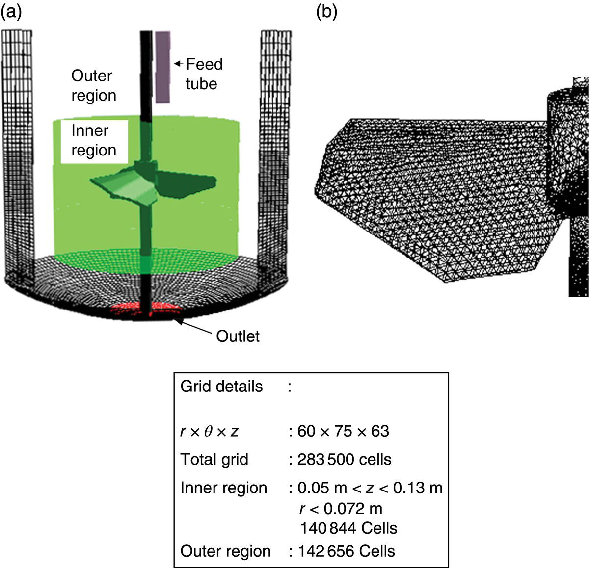
FIGURE 13.19 Solution domain and computational grid. (a) Solution domain. (b) Grid distribution on impeller blade.
Source: Reprinted with permission from Khopkar et al. [66]. Copyright 2004 The Institution of Chemical Engineers, Published by Elsevier B.V.

FIGURE 13.20 Comparison of predicted exit age distribution with ideal CSTR.
Source: Reprinted with permission from Khopkar et al. [66]. Copyright 2004 The Institution of Chemical Engineers, Published by Elsevier B.V.
Khopkar et al. [66] then numerically simulated various inlet and outlet configurations of the same vessel. Particle streak lines were simulated by releasing neutrally buoyant tracer particles from the inlet pipe. The simulated particle streak lines (for a flow time of five seconds) for different configurations are shown in Figure 13.21. Particle streak lines shown in Figure 13.21 help in understanding the complex interaction of incoming feed with impeller‐generated flow and outlet.

FIGURE 13.21 Streak lines for incoming liquid feed for different inlet/outlet configurations. (a) Inlet at the top and outlet at the bottom, N = 360 rpm. (b) Inlet at the top and outlet as overflow, N = 360 rpm. (c) Inlet at the bottom and outlet as overflow, N = 360 rpm. (d) Inlet at the bottom and outlet as overflow, N = 720 rpm.
Source: Reprinted with permission from Khopkar et al. [66]. Copyright 2004 The Institution of Chemical Engineers, Published by Elsevier B.V.
Khopkar et al. [66] used quasi‐steady‐state approach with multiple snapshots for simulating the flow in an industrial continuous flow stirred tank reactor. They observed that multiple numbers of snapshots are needed to adequately represent the flow generated by an impeller and the interaction of the incoming liquid jet with the impeller would depend on the design of the impeller. They further recommended that after establishing the flow, detailed species transport equations with any one of the snapshots could be used for simulating RTD at the outlet. However, the mixing simulation with quasi‐steady‐state approach does not accurately capture the interaction of the incoming jet with the rotating impeller, but the obtained results are found to be sufficient for the “a priori” suggestion for the evaluation of the different design configuration.
13.3.1.3 Viscous Mixing
Formulations are widely used in pharmaceutical, paint, food, polymer, and personal care products. Some of the most difficult mixing problems do get encountered in making these formulations. In many situations these formulations exhibit highly viscous, non‐Newtonian, and viscoelastic fluids. With all non‐Newtonian fluids, the potential exists that a portion of a tank will remain unmixed because of inadequate fluid motion. Because of both the high viscosity and non‐Newtonian behavior, special equipment is often required for mixing.
Mixing can be brought about in viscous systems only by mechanical action or by the forced shear or by elongational flow of the matrix. Mixing achieved through the history of deformation imparted to the fluid is called distributive mixing. In distributive mixing the homogeneity of the mixture can be quantified through the scale of segregation [67], whereas in dispersive mixing a consequence of the history of the fluid mechanical stresses is imposed on the mixture for breakup of agglomerates and drops. A dispersive mixing index can be quantified through strength of the pure elongational flow. The interrelationship between dispersive and distributive mixing is illustrated in Figure 13.22. In general, viscous mixing operations require some combination of dispersive and distributive actions. Before explaining some examples of viscous mixing, basic definitions of distributive and dispersive mixing are explained in the following subsection. These definitions will help in quantifying mixing in the process equipment.

FIGURE 13.22 Schematic illustration of distributive and dispersive mixing. (a) Bad dispersion and bad distribution. (b) Bad dispersion and good distribution. (c) Good dispersion and bad distribution. (d) Good dispersion and good distribution.
13.3.1.3.1 Measures of Distributive and Dispersive Mixing
As said earlier the purpose of the distributive mixing is to create uniform macrostructure. It is created due to the presence of chaotic motion in the deterministic laminar flows [68]. A variety of tools have been developed to examine and characterize chaotic flows including Poincare sections, periodic point analysis [69], and stretching distributions [70]. These tools do provide rich insight into the nature of chaotic flows and reveal the mechanism of chaotic mixing, but do not provide tools to quantify the distributive mixing behavior. Tucker III and Peters [71] numerically simulated mixing in a 2D time‐periodic flows in a rectangular cavity with upper and lower moving walls (see Figure 13.23). The mixing pattern was simulated using mapping method, which has a finite spatial resolution and certain amount of numerical diffusion. A variety of protocols involving time‐periodic sliding motions of the upper and lower cavity surfaces were studied. For quantifying distributive mixing, two measures of distributive mixing were proposed and examined: the standard deviation among samples σ and the maximum sample error E. Both these measures are closely related to the distributive mixing and small value of either means that the cell concentrations are nearly uniform:


where
- Vavg is the averaging volume.
- cavg is the final uniform concentration.
- L is the length scale of the averaging volume.
- M is the number of points in the mixer separated by the distance L.

FIGURE 13.23 Eight example mixtures simulated by Tucker III and Peters [71] using mapping method. (a) A8. (b) B8. (c) D2. (d) C8. (e) D4. (f) C16. (g) E8. (h) B16.
Source: Reprinted with permission from Tucker and Peters [71]. Copyright 2003 Korean Society of Rheology and Australian Society of Rheology.
Tucker III and Peters [71] observed that E and σ both provide the ability to compare the mixture patterns that may be quite different in appearance and to say which mixture is better distributed.
Dispersive mixing is usually more difficult to achieve than the distributive mixing. Dispersive mixing involves breakup of agglomerates and droplets in flow, caused by stresses large enough to overcome the cohesive or interfacial forces that tend to keep the agglomerates or the droplets intact. Two main mechanisms are responsible for dispersive mixing, viz. shear flow and elongational or extensional flow. Quantitative studies of droplet breakup in simple shear and pure elongational flows have shown that the elongational flow is more effective than the simple shear flow especially in the case of high viscosity ratios and low interfacial tensions. This is been clearly explained in Figure 13.24 where the Weber or capillary number is plotted again the viscosity ratio. Based on Figure 13.24, the minimum dispersed phase drop radius can be achieved where the viscosity p is close to unity, but the dispersion by shear flow is not possible if p exceeds 4. This limit could be different for viscoelastic fluids.
FIGURE 13.24 Critical Weber number versus viscosity ratio.
Source: Reprinted with permission from Grace [72]. Copyright 1982 Gordon and Breach Science Publisher Inc.
Accurate estimation of dispersive mixing efficiency would involve tracking of the dispersed phase during their entire residence time in the equipment and following the dynamics of their breakup and coalescence. However, such approach is numerically very expensive. A simpler global approach is required, which will help in discriminating between various designs and processing conditions for effective mixing equipment selection. A flow field characteristic relevant to dispersive mixing is known as flow strength [73, 74]. The flow strength is function of rate of deformation tensor and Jaumann time derivative of rate of deformation tensor. The flow strength parameter ranges from zero for pure rotational fluid to infinity for pure elongational flow; its value is unity for simple shear flow. However, numerically determining flow strength for complex geometry is difficult. Yang and Manas‐Zloczower [75] defined dispersive mixing index λ that quantifies the relative strength of the pure elongational flow component:
where
- |D| and |ω| are the magnitudes of the rate of strain and vorticity tensors, respectively.
The above parameter assumes values between 0 for pure rotation and 1 for pure elongation, with a value of 0.5 for simple shear. This mixing index is not frame invariant, but still can be used as first approximation to discriminate between various equipment designs and processing conditions [75, 76].
13.3.1.3.2 Examples of Viscous Mixing
It has been well established that the chaos is necessary for achieving efficient mixing in laminar stirred vessel [77]. Chaotic mixing is characterized by the exponential rate of stretching and folding of fluid elements. To illustrate this, Arratia et al. [78] used the planar laser‐induced fluorescence (PLIF) snapshot through the axis of the mixing tank filled with Newtonian fluid and stirred with concentric disks and Rushton turbines. Figure 13.25a demonstrates that the fluid does not mix down to a very small length scale. No sign of chaotic mixing was observed. Flow was characterized by a linear rate of stretching. Later, they induced chaos in the system by replacing the disk by Rushton turbines. They found out that the passage of blades periodically perturbed the flow and triggered the stretching and folding of fluid material, which helped in achieving efficient mixing (Figure 13.25b).

FIGURE 13.25 Chaotic mixing in stirred tank. (a) Flow generated by axisymmetric disk. (b) Flow generated by Rushton turbine.
Source: Reprinted with permission from Arratia et al. [78]. Copyright 2006 American Institute of Chemical Engineers.
Zalc et al. [79, 80] used the computational model for simulating the chaotic mixing in the stirred vessel equipped with multiple Rushton turbines. They computed flow field using the ORCA software (Fujitsu, Campbell, CA). Extensive comparison of simulated results was done with the PIV and PLIF measurements. Figure 13.26 shows the comparison of experimentally measured flow field with numerical results. CFD results accurately predicted size and location of the poorly mixed regions in the stirred vessel. Zalc et al. [79, 80] carried out quantitative measure of mixing intensities in chaotic flows by computing the accumulated stretching of small fluid filaments. These simulations were performed by placing small vectors in the flow. The deformation of each infinitesimal vector by the instantaneous velocity gradient along its trajectory while being convected throughout the flow domain was calculated for quantifying stretching value (λ). Figure 13.27 illustrates the stretching field for the different Reynolds number values 20, 40, and 160 after 20 revolutions. The contour maps reveal the heterogeneity of stretching and subsequently help in identifying poor mixing regions in the stirred vessel. The contour plot also shows the change in the poor mixing region structure with impeller Reynolds number. A priori knowledge of such stretching distribution pattern not only helps in identifying the poor mixing regions but also provides guideline in deciding the injection point for additives to achieve optimum distribution.
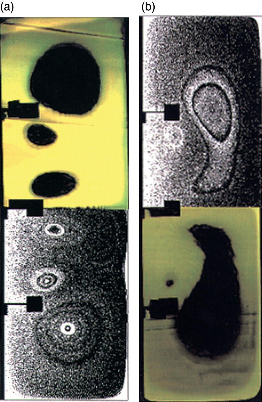
FIGURE 13.26 Comparison of experimental and simulated flow field results in stirred vessel equipped with three Rushton turbines. (a) Re = 20. (b) Re = 40.
Source: Reprinted with permission from Zalc et al. [80]. Copyright 2002 American Institute of Chemical Engineers.
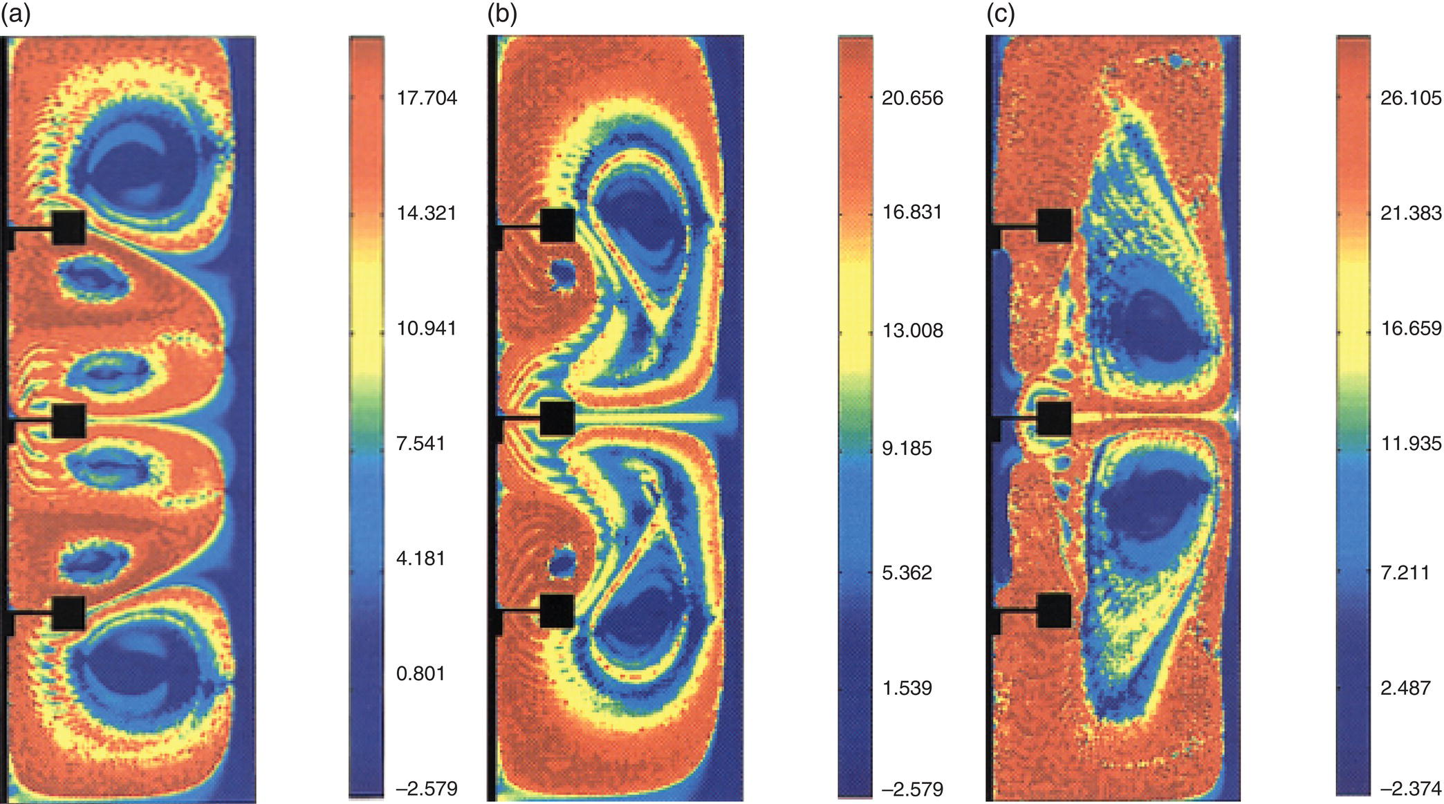
FIGURE 13.27 Simulated stretching field at 20 seconds for different Reynolds numbers. (a) Re = 20. (b) Re = 40. (c) Re = 160.
Source: Reprinted with permission from Zalc et al. [80]. Copyright 2002 American Institute of Chemical Engineers.
In order to improve the chaotic mixing, few approaches were suggested in literature, viz. using variable agitation speed instead of constant agitation by Szalai et al. [81], using eccentrically mounted impellers [77, 78, 82], and using dual shaft mixers [83]. Cabaret et al. [83] experimentally studied the mixing kinetics in a laminar flow stirred vessel equipped with multiple Rushton turbines. They used color discoloration method for quantifying the mixing in vessel. They observed that the mixing in a dual shaft stirred vessel is more efficient in comparison with centrally mounted shaft and off‐centered shaft systems (see Figure 13.28 for details). Dual shaft system also provides an additional degree of freedom, i.e. direction of rotation for influencing prevailing fluid dynamics. Cabaret et al. [83] observed better mixing in counterrotating mode as compared with corotating mode of operation.

FIGURE 13.28 Mixing analysis of stirred vessel. Mixing systems (a) single shaft configuration. (b) Dual shaft configuration. (c) Mixing analysis for various configurations.
Source: Reprinted with permission from Cabaret et al. [83]. Copyright 2007 The Institution of Chemical Engineers, Published by Elsevier B.V.
Nowadays, the industry needs impellers that can work in laminar, transitional, or turbulent regimes with minimum modifications. Standard agitators like close‐clearance and open impellers exhibit some limitations with this aspect. On one hand, close‐clearance impellers such as helical ribbons have a good distributive mixing performance in laminar regime. However, this situation is completely reversed when the condition changes from laminar to transitional or turbulent. Also, they do not generate sufficient dispersive mixing that is essential for improving mixing on smaller scale. On the other hand, open impellers like the Rushton turbine or pitched blade turbine are known to be very efficient at high Reynolds number, but in laminar regime, segregated zones are produced. The situation becomes critical if along the process time the phases to be mixed develop non‐Newtonian rheological properties such as shear thinning.
Recently, several innovative strategies have been proposed to tackle this problem. Multi‐shaft mixers with bulk flow impeller mounted on one shaft and open impeller or high‐shear mixer mounted on second shaft provide freedom in achieving desired level of mixing (see, for example, Refs. [84–87] and so on). The main idea is simple – association of different classes of agitators rotating at different speeds. In this way it is possible to create a mixer that achieves the process objectives – “blending” the capabilities of several agitators. At the end, a dynamic mixing unit that adapts with the process necessities is obtained. Scaling up of these equipments is still a challenge as not sufficient experimental data is available in the literature. Also, the available data does not cover all the possible degrees of freedom available with the designs of the multi‐shaft mixers. Validated CFD model can help us in filling these gaps with the experiments. Rivera et al. [86] simulated flow in a coaxial mixer using POLY3DTM (Rheosoft, Inc.). They simulated the flow generated in a coaxial mixer equipped with anchor impeller on one shaft and Rushton turbine on second shaft. They correlated the quality of distributive and dispersive mixing with the ratio of flow number Nq and head number Nh. Their results suggest that the corotating mode has better distributive mixing than counterrotating mode for both Newtonian and non‐Newtonian fluids (see Figure 13.29). They also observed that the predicted value of ratio Nh/Nq is smaller for corotating mode as compared with counterrotating mode (see Ref. [86] for more details).
FIGURE 13.29 Simulated viscosity profile for non‐Newtonian fluid in coaxial mixer. (a) Corotating mode. (b) Counterrotating mode. (c) Single Rushton turbine.
Source: Reprinted with permission from Rivera et al. [86]. Copyright 2005 Elsevier Ltd.
13.3.2 Solid–Liquid Mixing
In the manufacturing process of pharmaceutical intermediates, often handling of slurry will occur at some point. Typical solid–liquid mixing operations in the pharmaceutical industry are crystallization, dispersion, and dissolution. The process requirements of all these processes are different, and they have different challenges. Dispersion of solids is a physical process where solid particles or aggregates are suspended and dispersed by the action of an agitator in a fluid to achieve a uniform suspension or slurry. In dissolution process, solid particles are reduced in size and ultimately disappear as they are incorporated as solute in the liquid. However, in leaching process, a soluble component of the solid dissolves and left with particles of having different size, density, and/or porosity. The density and viscosity of the resulting liquid may differ considerably from the original liquid for some systems. In both dispersion and in some dissolution application, incorporation of solids is very challenging. However, crystallization and precipitation start with a solid‐free liquid phase if unseeded, and the solid particles form during the operation. The solids grow in size as well as in population. The viscosity and density of the slurry thus formed usually changes. The process goals include control of the rate of nucleation and growth of the particles as well as the minimization of particle breakage or attrition. Both the average size and the particle size distribution are important properties. Liquid‐phase mixing to achieve uniformity of supersaturation or to avoid local high concentration regions is important in achieving particle size control. In the following subsections, computational modeling of stirred slurry reactor is explained in detail with context to crystallization, dispersion, and dissolution processes.
13.3.2.1 Crystallization in Stirred Vessel
In pharmaceutical industry, crystallization and precipitation are widely used processes in manufacturing of various drug molecules. Precipitation and crystallization refer to unit operations that generate a solid from a supersaturated solution. The nonequilibrium supersaturated condition can be induced in a variety of ways such as removal of solvent by evaporation, addition of another solvent, changes of temperature or pressure, addition of other solutes, oxidation–reduction reactions, or even combinations of these. The distinction between precipitation and crystallization is quite often based on the speed of the process and the size of the solid particles produced. The term precipitation commonly refers to a process that results in rapid solid formation that can give small crystals that may not appear crystalline to the eye, but still may give very distinct X‐ray diffraction peaks. Amorphous solids (at least as indicated by X‐ray diffraction) may also be produced through precipitation. The term precipitation also tends to be applied to a relatively irreversible reaction between an added reagent and other species in solution, whereas crystallization products can usually be redissolved using simple means such as heating or dilution. Precipitation processes usually begin at high supersaturation where rapid nucleation and growth of solid phases occur. In both precipitation and crystallization processes, the same basic steps occur: supersaturation, nucleation, and growth.
Supersaturation affects both crystal growth and nucleation rates, which in turn impact the particle size distribution. A higher level of nucleation leads to smaller particles and vice versa. Also, a high degree of nucleation rate over crystal growth rate due to a high degree of supersaturation can lead to poorer rejection of impurities [88]. Nucleation does not necessarily begin immediately on reaching a supersaturated condition, except at very high supersaturation, and there may be an induction period before detection of the first crystals or solid particles.
Tung [88] used these time scales with the liquid‐phase mixing time for explaining complexity of the process. He defined two dimensionless numbers, viz. Danucleation and Dacrystallization:
where
- τmixing is the mixing time.
- τinduction is the induction time for primary nucleation.
- τrelease of supersaturation is the time required to release the supersaturation.
Danucleation ≪ 1 means a complete mixing before the nucleation is achieved. Similarly, Dacrystallization ≪ 1 means a complete mixing is achieved before the supersaturation is released. This would be the case for crystallization with relatively slow crystallization kinetics in releasing the supersaturation. Since the order of mixing time in a crystallizer is generally available, it is straightforward to learn if the crystallization system could be sensitive to mixing by comparing the induction time for nucleation or time for release of supersaturation. This suggests that the liquid‐phase mixing time plays a very important role in the crystallization.
It is important to recognize the influence of mixing on the product characteristics. In general mixing is defined at three scales, viz. macromixing, mesomixing, and micromixing. Macromixing is defined on the scale of the vessel, mesomixing is defined in context of dispersion of the antisolvent plume at the feed point, and micromixing determines the mixing at the molecular level and influences the induction time. Micromixing is influenced by the impeller type and speed plus relative location of the antisolvent feed pipe with respect to impeller. Thus, feed pipe location, pipe diameter, and antisolvent flow can impact both micromixing and mesomixing times. For example, when the antisolvent feed rate is faster than the local mixing rate, resulting in a plume of highly concentrated antisolvent that is not mixed at the molecular level. This can yield a high localized nucleation rate. This will present scale‐up difficulties, requiring a thorough engineering analysis for success.
The modeling of well‐mixed crystallizers involves the computation of the PBE together with the material balance equations for each species in solution. Numerous numerical techniques that compute the full crystal size distribution (CSD) have been used to model well‐mixed batch, semi‐batch, or continuous crystallizers. In most of the studies, the actual prevailing mixing condition was not simulated and is approximated with ideal mixing behaviors. For a more realistic simulation, it is necessary to solve the standard momentum and mass transport equations together with the PBE coupled flow simulation. Rielly and Marquis [89] provided an explanation on the pivotal role of fluid dynamics on the kinetics of crystallization and resulting CSD. Figure 13.30 explains how different scales of crystallizer fluid dynamics influence the crystallization process. Rielly and Marquis [89] built a computational model where particle or crystal motion was simulated in Lagrangian framework. They observed that the crystal particle experiences region with very different micro‐flow properties and it can be explained through the variation in the distribution of instantaneous slip velocities. They also concluded that the distribution of the variation in slip velocities experienced by the crystals is strongly dependent on the particle microscale and macroscale Stokes number defined by the two flow time scales, viz. lifetime of turbulent eddy and circulation time or mixing time. They also observed that neglecting the effects of microscale flow properties significantly reduces the variance of the macroscale time scale.

FIGURE 13.30 Suspension fluid dynamics effect on the crystallizer kinetics.
Source: Reprinted with permission from Rielly and Marquis [89]. Copyright 2001 Elsevier Science Ltd.
In all the studies available on the CFD modeling of crystallizer, the presence of solids is modeled by treating the slurry as a pseudo‐homogeneous fluid with a spatial distribution of effective viscosity that depends on the local solid fraction. Thus, they do not exactly simulate the flow essential for estimating accurate microscale flow properties that will further influence the macroscale flow time scales. There are multiple reasons for not yet development of a comprehensive computational model for simulating whole crystallization process. First, the computational model for simulating hydrodynamics of slurry is not yet fully validated. Second, although certain progress has been made in simulating micromixing effect on the crystallization kinetics, other mechanisms such as secondary nucleation, agglomeration, and breakage are yet to be modeled and validated. Third, most important reason is huge computational requirement for coupling algorithms of multiphase flow and crystallization kinetics. It is therefore necessary to validate these models separately and develop an innovative approach for combining the results of these models for effective design of crystallization process.
13.3.2.2 CFD Simulation of Solid Suspension in Stirred Vessel
In the previous section a detailed discussion on the computational modeling of stirred slurry reactor is presented. The developed model was evaluated by comparing results for solid volume fraction profiles averaged over reactor cross section. A close look at the prevailing fluid dynamics in the crystallizer shows very complex behavior. The average density and viscosity continuously changes due to formation and growth of solids. There is a possibility of solid suspension mechanism demonstrating various transient phenomena in crystallizer. These transients will definitely influence the transport processes. It is therefore necessary that the computational model must predict the transients associated with the slurry suspension and its implications on the liquid‐phase mixing. Sardeshpande et al. [90] observed the hysteresis in the suspension quality with respect to impeller speed. Figure 13.31 shows the visual observation of hysteresis observed by Sardeshpande et al. [90]. Their data also suggest that the observed hysteresis is more profound at higher solids loading.
FIGURE 13.31 Visually observed cloud height hysteresis.
Source: Reprinted with permission from Sardeshpande et al. [90]. Copyright 2010 American Institute of Chemical Engineers.
Sardeshpande et al. [90] used computational model with different interphase drag force formulations for simulating the sudden hysteresis observed in cloud or suspension height. Figure 13.32 shows the comparison of the cloud height predicted using Brucato et al. [21] drag law and modified Brucato's drag law recommended by Khopkar et al. [38]. They observed that for both increasing and decreasing impeller rotational speed, the computational model with Brucato's drag law overpredicted the cloud height. However, the computational model recommended by Khopkar et al. [37] reasonably captured the cloud height for both increasing and decreasing impeller rotational speed conditions. Ability of computational model to predict hysteresis enhances the capability of process engineer for a priori controlling the performance of slurry reactor, where small deviation in the suspension quality could influence the final product properties through different rates of transport and mixing rates as well as different particle–particle interaction.

FIGURE 13.32 Predicted cloud height hysteresis using two drag formulations. (a) Brucato's drag coefficient. (b) Modified Brucato's drag coefficient suggested by Khopkar et al.
Source: Reprinted with permission from Sardeshpande et al. [90]. Copyright 2010 American Institute of Chemical Engineers.
13.3.2.3 Solid Suspension and Mixing in Stirred Reactor
Liquid‐phase mixing is quite important in many solid–liquid reactions as well. It not only affects the selectivity of reactions but also controls the temperature distribution inside the reactor for exothermic reactions. In many cases, stirred reactors are operated with higher solids loading (solid volume fraction >5.0%). In such situations, the liquid‐phase mixing process was found to show a complex interaction with the suspension quality (for example, Ref. [91]). A computational model, which is able to predict suspension quality and its influence of liquid‐phase mixing, will definitely help reactor engineers to obtain optimum performance of stirred slurry reactors. Recently, Kasat et al. [92] simulated liquid‐phase mixing in a stirred reactor for different operating conditions. Their simulations are reproduced here to explain the liquid‐phase mixing in a stirred slurry reactor.
The simulations are carried out in the experimental setup of Yamazaki et al. [38] with solid volume fraction equal to 10.0% and particle diameter equal to 264 μm. The simulations are carried out for 10 different impeller rotational speeds starting from 2 to 40 rps. The completely converged solid–liquid flow simulations were used to simulate liquid‐phase mixing. Mixing simulations were carried out with 1.0% (by volume) of tracer, having same physical properties of liquid in the vessel. The tracer history was recorded at eight different locations. In stirred slurry reactor, delayed mixing was usually observed near the top surface of the liquid. Therefore, tracer history was recorded at four different locations close to top surface (Ref. [92] for more details). The mixing time in the present work is defined as the time required for the tracer concentration at these locations to lie within ±5.0% of the final concentration (C∞).
It will be very helpful to first shed light on the predicted suspension quality before discussing the influence of suspension quality on the mixing process. In a stirred slurry reactor, the critical impeller speed for complete off‐bottom suspension Ncs and complete suspension Ns are two very important design parameters. The concepts of critical impeller speed were introduced more than 40 years ago and are primary design parameters used even today by reactor engineers for scale‐up and design of stirred slurry reactor. The predicted suspension quality was analyzed to estimate the Ncs and Ns. Several criteria are available in the literature to determine the values of Ncs and Ns. However, those criteria are applicable for experimental measurements and cannot be extended directly to the CFD simulations with the EE approach. Bohnet and Niesmak [93] have proposed alternative criteria based on the standard deviation σ of solid concentration to describe the suspension quality (see Eq. (13.17)). The same criterion is used in the present work to describe the suspension quality. The decrease in standard deviation value is manifested as an increase in the quality of the suspension. Based on the range of the standard deviation, the quality of the suspension is broadly divided into three regimes: homogeneous suspension, where the value of the standard deviation is smaller than 0.2 (σ < 0.2); complete off‐bottom suspension, where the value of the standard deviation lies between 0.2 and 0.8 (0.2 < σ < 0.8); and incomplete suspension, where the standard deviation value was found to be higher than 0.8 (σ > 0.8). This criterion enables the prediction of Ncs and Ns and also gives the information on quality of suspension prevailing in the vessel.
The standard deviation values were estimated from the predicted solid volume fraction for all the 10 simulations carried out at different impeller rotational speeds. It must be noted that solid volume fraction values at all computational cells were used to estimate the standard deviation value. The predicted variation of standard deviation values with respect to impeller speed is shown in Figure 13.33. It can be seen from Figure 13.33 that three distinctly different suspension conditions, viz. incomplete suspension, complete off‐bottom suspension, and homogeneous suspension, can be identified in the vessel. At a lower impeller speed, the computational model predicted very high values of the standard deviation (σ > 0.8), indicating incomplete suspension in the vessel. It is also observed that the standard deviation values drop sharply with an increase in the impeller rotational speed until complete off‐bottom condition is achieved. The computational model predicted standard deviation value equal to 0.7 for 15 rps. This indicates the presence of a critical impeller speed for complete off‐bottom suspension (σ = 0.8) close to 15 rps. This is in good agreement with the Ncs (= 13.4 rps) estimated using correlation proposed by Zwietering [94] for the experimental setup of Yamazaki et al. [38]. With further increase in the impeller rotational speed, the values of standard deviation drop slowly till the system achieves homogeneous suspension condition. The predicted results suggest that the homogeneous suspension condition for the experimental condition of Yamazaki et al. [38] is achieved at impeller speed Ns equal to 40 rps (σ = 0.17).
FIGURE 13.33 Predicted influence of impeller rotational speed on suspension quality, for dp = 264 μm and α = 0.1.
Source: Reprinted with permission from Kasat et al. [92]. Copyright 2008 Elsevier Ltd.
The species transport simulations are then carried out to understand the mixing process in the experimental setup of Yamazaki et al. [38]. The variation of predicted dimensionless mixing time (Ntmix) with impeller rotational speed is shown in Figure 13.34. It can be seen from Figure 13.34 that the dimensionless mixing time first increases sharply with increase in the impeller rotational speed and then drops slowly with further increase in impeller speed. Figure 13.34 shows minimum value of dimensionless mixing time for lowest impeller speed (2 rps). The predicted liquid velocity vector plot was studied to understand the possible reason behind the observance of a minimum mixing time. The predicted flow characteristics for an impeller rotational speed equal to 2 rps are shown in Figure 13.35. It can be seen from Figure 13.35a that the computational model predicted single‐loop velocity pattern in the vessel. It is possible that for such a low impeller speed, impeller action is not sufficient to lift the particles from the vessel bottom (see Figure 13.35b). The solid bed present at the bottom of the reactor might offer apparent low off‐bottom clearance to the impeller‐generated flow and therefore lead to single‐loop flow pattern for Rushton turbine. In such a scenario, all the energy dissipated by the impeller becomes available for generating liquid circulations in the vessel and for fluid mixing. Therefore, it is possible to have faster mixing in the reactor at low impeller rotational speed.

FIGURE 13.34 Predicted influence of impeller rotational speed on the dimensionless mixing time, for dp = 264 μm and α = 0.1.
Source: Reprinted with permission from Kasat et al. [92]. Copyright 2008 Elsevier Ltd.

FIGURE 13.35 Predicted influence of impeller rotational speed on the liquid‐phase flow field, for dp = 264 μm and α = 0.1. (a) N = 2 rps. (b) N = 5 rps.
Source: Reprinted with permission from Kasat et al. [92]. Copyright 2008 Elsevier Ltd.
With increase in impeller rotational speed, the dimensionless mixing time increases, reaches maxima, and then drops slowly (see Figure 13.34). In the present work, the maximum in the mixing time was found to happen at around 5 rps. At 5 rps the impeller‐generated flow becomes sufficient to start suspending solids into the bulk volume of the reactor. The energy dissipated by the impeller is now distributed for generating liquid circulations and fluid mixing and suspending the solids. The single‐loop flow pattern changes to the classical two‐loop structure for the Rushton turbine. The part of the energy dissipation for solid suspension and the rate of exchange between the two loops contribute to the slower mixing in the vessel for the 5 rps condition. A further increase in the impeller rotational speed leads to a reduction in the mixing time (increase in the mixing efficiency). This observed reduction in the mixing time continues till the system achieves the complete off‐bottom suspension condition (i.e. Ncs = 15 rps). The operating conditions (impeller rotational speed) after Ncs show a gradual decrease in the mixing time with an increase in impeller rotational speed. The present simulations also supported the operating range at which maxima of mixing time occur, i.e. N = Ncs/3 [91].
The simulated results are further analyzed to understand the mixing in the stirred slurry reactor. The predicted tracer histories in the bulk volume of reactor (more close to impeller) and near the top surface of vessel were compared. The comparison of predicted tracer histories is shown in Figure 13.36. It can be seen from Figure 13.36 that the homogenization process is much faster in the region close to impeller compared with the region near the top surface. It was also observed that the difference between the top region and the impeller region is strongly dependent on the suspension quality present in the vessel. Figure 13.36 shows that in incomplete suspension and in complete off‐bottom suspension conditions, the time required for the homogenization near the top surface is significantly high compared with the time required for homogenization close to the impeller. The difference decreases as the system approaches the homogeneous suspension condition. Kasat et al. [92] showed that the lower liquid velocities present in the clear liquid layer above the solid cloud is responsible for the slower mixing process.

FIGURE 13.36 Predicted influence of suspension quality on delayed mixing in the top clear liquid layer, for dp = 264 μm and α = 0.1.
Source: Reprinted with permission from Kasat et al. [92]. Copyright 2008 Elsevier Ltd.
Preceding subsections discuss mixing issues in gas–liquid and solid–liquid systems. Similar approach can be used for addressing issues in other systems like liquid–liquid or gas–liquid–solid stirred vessels. Apart from predicting dispersion or suspension quality and mixing time, CFD models allow estimation of circulation time distribution, different zones in stirred vessels with different prevailing shear rates, interaction of impeller stream with inlet and outlet nozzles, and so on. It is possible to creatively use information obtainable from CFD to gain better insight and support engineering decision making. For example, information on different shear zones and RTD in these different zones often provides used clues for quantifying influence of scale on “breakup” and “coalescence” dominated zones. It is not possible to discuss actual industrial cases here for the sake of protecting confidential information. It is however hoped that information provided here will allow resourceful engineer to develop appropriate computational flow models and use the simulated results for addressing practical design and scale‐up issues.
13.3.2.4 CFD Simulation of Antisolvent Crystallization
Pharmaceutical and fine chemical makers frequently rely on antisolvent crystallization, also known as precipitation for generating solid from a solution in which the product has high solubility. This technique is used for a variety of applications such as polymorph control, purification from a reaction mixture, and yield improvement. Antisolvent crystallization achieves supersaturation and solidification by exposing a solution of the product to another solvent (or multiple ones) in which the product is sparingly soluble. Although this technique has the potential to achieve a controlled and scalable size distribution, it is not without problems. The product requires purification or separation steps to remove the antisolvent(s).
Woo et al. [95] discussed the model development in the framework of CFD for simulating the effect of mixing on the antisolvent crystallization process. In the CFD model they included PBE for the evolution of the CSD and the PDF of the local turbulent fluctuations. In addition to that, they used separate sub‐models for nucleation and growth kinetics and Einstein equation for modeling effect of solid concentration on the rheology. For detail model equations and its implementation, please refer to Woo et al. [95]. Computational model was then used to predict the evolution of volume‐averaged antisolvent, mass percent, supersaturation, nucleation rate, and mean growth rate. While comparing with the earlier published experimental observations, Woo et al. [95] found that the computational model was able to simulate temporal evolution of nucleation and growth rates at the inlet. They also predicted higher growth rates at the impeller region due to higher turbulence (Figure 13.37). They attributed this to improved mass transfer. This improved mass transfer at higher impeller rotational speed consequently led to faster desupersaturation, which resulted in lowering overall nucleation rate. Its impact on the overall crystallization process is explained through predicted final CSD. Figure 13.38 shows the predicted CSD at the end of one hour for three different rotational speeds. The predicted results show that fewer and slightly larger crystals were obtained for higher agitation rate. These results are qualitatively in agreement with the experimental findings.

FIGURE 13.37 Simulated spatial distributions of process parameters for antisolvent crystallization at different time intervals. (a) Spatial distribution of the antisolvent mass fraction. (b) Spatial distribution of the supersaturation. (c) Spatial distribution of the nucleation rate. (d) Spatial distribution of the mean growth rate.
Source: Reprinted with permission from Woo et al. [95]. Copyright 2006 American Chemical Society.

FIGURE 13.38 Simulated volume‐averaged crystal size distribution for different impeller rotational speed.
Source: Reprinted with permission from Woo et al. [95]. Copyright 2006 American Chemical Society.
Woo et al. [95] then used the computational model for simulating antisolvent crystallization with reverse mode of addition. Figure 13.39a shows the predicted final volume‐averaged CSD. As anticipated, the computational model predicted finer particle size with reverse mode of addition in comparison with the normal mode of addition. They also used computational model for predicting influence of scale of the equipment on the CSD. Figure 13.39b shows the comparison of the predicted CSD for different scale and different scale‐up criteria. The computational model predicted nonsignificant impact of scale of operation on the predicted CSD for constant power per unit volume that is consistent with the experimental findings by Torbacke and Rasmuson [96].

FIGURE 13.39 Simulated volume‐averaged crystal size distribution. (a) Predicted CSD for different addition mode. (b) Predicted influence of scale‐up on the CSD.
Source: Reprinted with permission from Woo et al. [95]. Copyright 2006 American Chemical Society.
13.3.2.5 Process Innovation in Crystallization
It is been known that by reducing drug particle size to the absolute minimum may lead to significantly improving drugs' wettability and bioavailability. This will require a small mean crystal size and a narrow size distribution. Normally, pharmaceutical powders are polydisperse, i.e. consisting particles of different sizes. Polydisperse powders create considerable difficulties in the production of dosage forms. Particles of monosize (equal size) may be ideal for pharmaceutical purposes. In practice, powders with narrow range of size distribution can obviate the problems in processing them further. Making such products demand continuous processing either through an in‐line mixer or via conducting milling on finished product [97]. At times milling technique can cause negative results such as dusting, caking, electrostatic charges, and in some times a polymorphic transformation. Process intensification by combining impinging jet reactor with stirred vessel (see Figure 13.40) provides an opportunity to control the final product particle size. It is been observed that uniform or nearly homogeneous nucleation happens in the impinging jet reactor [99]. These uniformly formed nucleates then feed into a stirred vessel where crystal growth or ripening will happen. Validated computational model not only will help in designing new innovative such systems but also will help in optimizing the operating parameters and mixing and transport processes for achieving desired process and product requirements.

FIGURE 13.40 Conceptual process intensification of antisolvent crystallization.
Source: Reprinted with permission from Genck [98]. Copyright Genck International.
13.3.2.6 Solid Suspension in Viscous Medium
There are several pharmaceutical suspensions available in the market. In these suspensions therapeutically active ingredients are uniformly dispersed in the medium. The solid particles used in these suspensions are smaller than 5 μm but have a tendency to settle. These suspensions are broadly differentiated into dilute suspensions (2–10% w/w) or concentrated suspensions (up to 50% w/w). It is imperative from the perspective of product specification to have uniform suspension in order to have the administration of a measured dose. Formulation experts avoid or minimize the settling either by reducing particle size or by increasing the viscosity of the continuous phase. Increasing the viscosity of the continuous phase is more predominantly used in formulations of these suspensions. The influence of rheology on solid suspension has received relatively less attention in the literature. Ibrahim and Nienow [100] showed that at higher viscosity, the Zwietering equation is likely to fail, with an error as large as 90%. The possible reason could be noninclusion of complex rheology behavior in the equation. It is known that in laminar condition, the presence of fine solids in the liquid produces shear‐thinning non‐Newtonian behavior [101].
Wu et al. [102] experimentally studied the influence of non‐Newtonian rheology on the characteristics of solid suspension in a mechanically agitated vessel. They studied the suspension of glass beads in water and Carbopol solution. Their experimental results are presented in Figure 13.41. Very interesting observations were made by Wu et al. [102]. They observed that adding 0.04% Carbopol in water resulted in the reduction in the just suspension speed of impeller (Njs) by 15%. They attributed this drop to the reduction in the settling velocity of the solids. They also observed that above 0.09% of Carbopol in water, the Njs sharply reduced to zero (Figure 13.41b). To explain this, the variation of settling velocity is plotted in Figure 13.41c for different viscosity values for glass beads having 100 μm diameter. It is seen that the settling velocity approaches to the few tens of μm/s for 0.09% Carbopol solution and hence will not see settling for longer time. In such situations, the definition of Njs becomes irrelevant in defining impeller operating conditions, and definition of effective dispersion becomes more relevant.

FIGURE 13.41 Influence of liquid‐phase viscosity on the suspension. (a) Bed height versus impeller rotational speed for water and 0.04% Carbopol solution. (b) Bed height versus impeller rotational speed for water and 0.04% Carbopol solution. (c) Effect of continuous phase viscosity on the settling velocity of glass particle, ρ = 2250 kg/m3 and dp = 100 μm.
Source: Reprinted with permission from Wu et al. [102]. Copyright 2001 John Wiley and Sons.
Handling solid dispersion in viscous medium is not an easy task. A complication that arises is that the fine particles (microscopic in size) maintain electrical and molecular attraction. These fine particles tend to lump together and form agglomerates that no amount of mixing will break. An aggregate (or agglomerate) is composed of a group of particles that are strongly adherent and can be broken down only by the application of relatively strong mechanical forces. In the days before the advancement of disperser, different mills were used in practice for reducing the size of the product. However, the processing was very time consuming and led to very long batch time. With the advent of the disperser, the de‐agglomeration process could be accomplished much more rapidly within the same vessel while mixing, resulting in a smoother, more uniform end product. The disperser is an impeller having thin disk with carefully designed teeth distributed radially about the circumference. Its action tears particles apart and disperses them uniformly throughout the product. This work is done with two actions: firstly, particles hitting the impeller are broken apart, or de‐agglomerated, and secondly, the intense turbulence surrounding the impeller causes particles to hit each other with great momentum and inertia. The energy of this impact physically breaks apart agglomerates. Figure 13.42 shows the commonly used disperser in the industry.

FIGURE 13.42 Different types of dispersers used in process industry. (a) Hi‐Vane impeller®, Morehouse Cowles. (b) R500® from Lightnin.
Disperser has very limited pumping capacity, and hence in a larger mixing vessel, it is imperative to use other flow impeller to continuously feed disperser for achieving better product results. In many industrial applications having high viscosity mixing, multi‐shaft impellers are widely used. In these systems, a close‐clearance impeller such as Anchor, Paravisc, or helical ribbon is mounted on the one shaft for facilitating distributive mixing, and single or multiple dispersers are mounted on the other shafts for dispersive mixing. Barar Pour et al. [103] studied the slurry blending in a dual shaft impeller system having continuous phase viscosity of 1 Pa·s and solid holdup of 10%. Figure 13.43 shows experimental setup of Barar Pour et al. [103]. They observed that the final particle size distribution is function of the disperser speed (see Figure 13.43b).

FIGURE 13.43 Slurry blending in a dual shaft stirred vessel. (a) Experimental setup. (b) Influence of deflo speed on the particle size distribution.
Source: Reprinted with permission from Barar Pour et al. [103]. Copyright 2007 The Institution of Chemical Engineers, Published by Elsevier B.V.
Empirical approach based on the experimental observation is still used in the designing of the mixing system for dispersing powdered solids in the viscous fluids. The dispersion process is itself very complicated and involves several stages – wetting, incorporation, agglomeration, and rupture. The current level of understanding on each of these stages is not sufficient. The experimental results of Barar Pour et al. [103] show different behavior of torque experienced by Paravisc impeller for different solids. The actual reason for this variation is not very clear. Also, the current level of understanding on agglomerate formation and its breakup in a complex flow is not up to the level of understanding of bubble and/or droplet coalescence and breakage. There are few studies reported in literature mainly by Manas‐Zloczower and coworkers [104–106], and Hansen et al. [107] presented models for simulating agglomerate breakup. Zeidan et al. [108] simulated the evolution of aggregates subjected to simple shear flow using a combined continuum and discrete model (CCDM). They solved the motion of discrete particles using Newton's second law of motion (DEM), and the continuum fluid flow was solved using locally averaged Navier–Stokes equations (CFD). This allowed Zeidan et al. [108] to study fully coupled aggregate deformation and breakup in a simple shear flow. They studied the breakage for aggregate having different cohesive strength. Figure 13.44 shows the simulated aggregate breakage for two different cohesive strengths. It can be seen that two different aggregate mechanisms exist. Weak aggregates rupture and at higher shear rate produce smaller and more uniform‐sized aggregates. However, erosion mechanism is dominant in breakage of strong aggregates, and it results in wider distribution.

FIGURE 13.44 Simulated aggregate rupture for different cohesive strengths. (a) Rupture of weak aggregates. (b) Erosion of strong aggregates.
Source: Reprinted with permission from Zeidan et al. [108]. Copyright 2007 The Institution of Chemical Engineers, Published by Elsevier B.V.
Cong and Gupta [109] used PELDOMTM software for simulating solid dispersion in a corotating twin‐screw extruder. The screws were rotated at 60 rpm, and 200 blue and 200 red segregated agglomerates were placed in the two halves of the twin‐screw extruder entrance. Quality of distributive mixing in a corotating twin‐screw extruder was evaluated by finding the change in the spatial distribution of initially segregated particles. Shannon entropy of mixture was first estimated, and then it was used for estimating color homogeneity index (CHI). CHI value lies between 0 and 1. Zero corresponds to completely segregated system, whereas one corresponds to completely mixed system. For the same twin‐screw extruder, quality of dispersive mixing was determined by using the erosion model of Scurati et al. [105]. In this model the rate of agglomerate size reduction is proportional to the shear rate and the difference between hydrodynamic (Fh) and cohesive (Fc) forces:
Please refer to Cong and Gupta [109] for more details on the definition of hydrodynamic and cohesive forces. Particle tracing scheme is used for the simulating particle motion. The change in the spatial distribution was determined by following the particle path lines to the desired axial location of the extruder. The predicted CHI for distributed and dispersive mixing is shown in Figure 13.45. It can be seen from Figure 13.45a that starting with completely segregated red and blue particles in each lobes, at z = 30 mm, the distribution of the particles in both the lobes is nonhomogeneous and the homogeneity improves with distance. At z = 90 mm, the particle distribution in the twin‐screw extruder is quite uniform. Initial guess of agglomerate and fragment radii determines the number of fragments erodes from the single agglomerate. For 0.5 and 0.11 mm for agglomerate and fragment radii, respectively, Alemaskin et al. [110] observed 93 fragments from a single agglomerate. Very high number of particles negatively influences the computational efficiency, and hence Cong and Gupta [109] in their simulations used 0.3 and 0.1 mm as the agglomerate and fragment radii, respectively. This led to 26 number of fragments resulting from erosion of single agglomerate. Figure 13.45b shows the spatial distribution of agglomerates and eroded fragments at three different locations of twin‐screw extruder. It shows that with only 400 agglomerates at entrance, the population of the fragments increases substantially with extruder length. They also observed that the CHI, which determines the mixing efficiency, improves significantly due to dispersive mixing. This suggests that alone simulating distributive mixing will not be sufficient for quantifying mixing efficiency in such applications.

FIGURE 13.45 Change in spatial distribution of solids due to distributive and dispersive mixing in a twin‐screw extruder. (a) With only distributive mixing. (b) Combined distributive and dispersive mixing.
Source: Reprinted with permission from Cong and Gupta [109]. Copyright 2008 Society of Plastics Engineers.
13.3.2.7 Solid Drawdown in a Stirred Vessel
In many practical applications, low density solids, more particularly powders, are added into the liquid. Powder addition is usually accompanied with a variety of problems, irrespective of whether powder is soluble or insoluble. Typical changes do happen during hydration of solids in liquid and are explained schematically in Figure 13.46. The first case is simpler case compared with rest of the three. The challenge in first case is to wet the surface of solids and incorporate them in the liquid if required without entraining air. However, in the remaining three cases, rheological challenges do crop up. For example, if the rate of dissolution is faster than the rate of surface wetting, then there is a possibility of having a high viscosity layer of liquid near the top surface. This layer will eventually cover the dry solids and may delay the further dissolution. If the liquid develops Bingham behavior, i.e. a yield stress, wetting will stop completely. Swelling of particles always results in a slower rate of wetting, which may even approach zero. Many food ingredients like starch and some proteins tend to swell in water; in general the particles may swell and/or dissolve in the liquid to various degrees (Figure 13.46). It is impossible to predict in general whether or not such behavior leads to a faster or slower rate of wetting, as compared with an unchanged bulk material.

FIGURE 13.46 Schematic illustration of typical changes taking place during hydration of powders. (a) Unchanged. (b) Dissolving. (c) Swelling. (d) Dissolving and swelling.
Source: Reprinted with permission from Schubert [111]. Copyright 1990 VCH Verlagsgesellschaft GmbH.
The rate of addition and surface motion can either worsen or improve powder addition. Many powders need to be added slowly enough that they do get sufficient time for wetting their surface and their incorporation into the liquid. Some hydrating thickeners such as cellulosic polymers need to be added quickly, while the fluid is still low viscosity and prevailing turbulence is there to provide aid in the addition and dispersion of the powder. This suggests that there is a specific rate of addition exists based on the wetting characteristics of the powders. Different mechanisms are recommended in the open literature for incorporating low density solids into the liquid in turbulent condition. Khazam and Kresta [112] identified three mechanisms of solid drawdown in stirred tanks: (1) Formation of stable single vortex (with no baffles or single baffle system) causes downward axial velocities at the surface responsible for drawdown. (2) Turbulent fluctuations form mesoscale eddies/vortices on the surface, which intermittently pull particles in the liquid. (3) Mean drag produced by the liquid circulation loops draw particles into the liquid where the downward axial velocities are greater than the particle slip velocity.
Most commonly used mechanism is generating a strong single vortex for incorporating solids (mechanism 1). The strong vortex can be generated using either no or partial baffling. Joosten et al. [113] used single baffle, Hemrajani et al. [114] used four baffles of width 1/50 tank diameter, and Siddiqui [115] recommended three partially immersed baffles 90° apart. Edwards and Ellis [116] found three‐blade marine propeller without any baffles to be the most energy‐efficient design. In this mechanism, during operation, headspace gas/air also gets entrained in the liquid. It is possible that in many practical applications, gas entrainment in the liquid needs to be avoided. This definitely puts challenge on the process engineer in designing the vessel and its operating conditions for efficient drawdown of the solids.
Several works have been reported in the past explaining the different baffling concepts and its implications on the drawdown of solids. It is well known that baffling suppresses the stable surface vortex formation and increases the intensity of mean drag and turbulence at the surface. This generates strong top‐to‐bottom liquid circulation. However, this circulation rapidly brings particles back to the surface. Hence researchers have recommended the partial or nonstandard baffling. Khazam and Kresta [112] experimentally and computationally studied the drawdown of the floating solids in a stirred vessel for two different baffle designs, viz. half baffles and surface baffles. Schematics of the different baffling configurations used by them are shown in Figure 13.47. The objective was to maintain a high level of turbulence at the surface while reducing the return circulation from the bottom of the tank. The performance of the baffle configurations was compared using the just drawdown speed, Njd, and cloud depth, CD, for the PBTD, PBTU, and A340 impellers. CFD simulations and measurements of the power number for the fully baffled and the surface baffled configurations were also reported. They found out that the drawdown speed for all the impellers was very similar for full and half baffles (see Figure 13.48). But with surface baffles, they found advantage in significant reduction in the drawdown speed Njd. They also observed that a more robust performance at large submergences and a better distribution of solids was obtained for the surface baffles.
FIGURE 13.47 Schematic of different baffle configurations studied.
Source: Reprinted with permission from Khazam and Kresta [112]. Copyright 2008 The Institution of Chemical Engineers, Published by Elsevier B.V.

FIGURE 13.48 Effect of baffle configuration on the Njd. (a) Up‐pumping pitched blade turbine. (b) Down‐pumping pitched blade turbine. (c) A340.
Source: Reprinted with permission from Khazam and Kresta [112]. Copyright 2008 The Institution of Chemical Engineers, Published by Elsevier B.V.
Atibeni et al. [117] used the PIV technique for elucidating the effect of baffle design on the drawdown of the floating particles. They observed that for the standard baffle system, just drawdown speed reduces by placing impeller off‐center. They observed more than 50% reduction in impeller power by this modification. They also found that around 50% impeller power reduces by modifying standard baffles with down triangle baffles. Hsu et al. [118] used both visual observations and CFD model for simulating the effect of impeller clearance and baffle design on the drawdown of the floating particles. They also observed positive impact of new baffle designs on the drawdown process over the standard baffles.
13.3.2.8 Solid Dissolution in Stirred Vessel
Solid dissolution is a common process unit operation during liquid mixing in the pharmaceutical industry. Incomplete dissolution can result in subpotent batches, resulting in batch failure. Competing elements such as the time required for dissolution versus the potential of microbial contamination over an extended mixing period may also be in play in a manufacturing setting. Dissolution in a stirred tank is influenced by many parameters. Khinast and coworkers [119, 120] provided an Ishikawa diagram (Figure 13.49) for explaining the various parameters that influence the operation. Many of these parameters cannot be changed in a pharmaceutical manufacturing setting. For example, most of the physicochemical properties of a raw material are fixed, although variations do occur due to the batch‐to‐batch variability of APIs. The process engineer has to work with process parameters, human environment, and equipment for improving the dissolution rate or time required for achieving complete dissolution. Other than the particle properties, the dissolution kinetics depend on the local mass transfer coefficient (which in turn is a function of suspension state and the local turbulence level), on the thermodynamics of the crystal, and on the equilibrium solubility at the fluid temperature.

FIGURE 13.49 Ishikawa diagram of mixing and dissolution of solids in liquid.
Source: Reprinted with permission from Adam et al. [119]. Copyright 2010 Elsevier B.V.
A key fluid dynamic parameter that will govern the dissolution time is the solid–liquid mass transfer coefficient. The rate of mass transfer is defined as
where
- k is the solid–liquid mass transfer coefficient.
- a is interfacial area.
- C* is the concentration at the interface that is saturation concentration.
- C is the concentration in the bulk liquid phase.
Thus by definition, achieving a constant mass transfer coefficient across different scales, one should achieve similar dissolution rates and hence similar dissolution times. In order to achieve constant mass transfer coefficients across different scales, it is important to know how the mass transfer coefficient is affected by different operating parameters.
Koganti et al. developed CFD model for simulating the dissolution of propylparaben in water for two different scales, viz. 2 L lab scale and 4000 L commercial scale. Their aim was to study the influence of scale‐up procedure on the dissolution process. They maintained the geometric similarity for both the scales, and operating conditions were scaled based on uniform power per volume. The predicted evolution of dissolution for both lab scale and commercial scale is shown in Figure 13.50. It shows that the difference between the laboratory scale and commercial scale is reasonably small and in order of 75–88% confidence for various operating conditions. It must be noted that the CFD simulation of dissolution process is only limited to the mass transfer where the model assumes perfectly wet condition for particles from the initial time. This is particularly because CFD models have not yet reached to the level where wetting by capillary action can be modeled with reasonable accuracy. However, they can be used for a priori predictions for evaluating influence of different design and process parameters.

FIGURE 13.50 Predicted results of solid dissolution in liquid. (a) Prediction of dissolution kinetics. (b) Comparison of time for 90% dissolution between lab and commercial scales.
Source: Reprinted with permission from Koganti et al. [121]. Copyright 2010 American Association of Pharmaceutical Scientists.
13.3.3 Tall Gas–Liquid Stirred Reactor: Flow and Mixing
In many industrial applications, tall vessels equipped with multiple impellers are used. The multiple‐impeller system provides better gas utilization, higher interfacial area, and narrower RTD in the flow system compared with a single‐impeller system. Also the multiple‐impeller systems are preferred in a bioreactor, as they offer lower average shear as compared with a single‐impeller system due to overall lower operational speed with nearly same power input. Overall, the tall stirred vessel offers more degrees of freedom for controlling the gas dispersion as well as the bulk flow of liquid phase. Different fluid dynamic characteristics can be obtained in a tall vessel depending on the equipment and the operating parameters, such as impeller design, impeller spacing, rotational speed, and volumetric gas flow rates. These different fluid dynamic characteristics lead to different rates of transport and mixing processes (see, for example, Refs. [122–126]). Khopkar et al. [126] and Khopkar and Tanguy [125] explained influence of operating conditions on mixing and influence of reactor hardware on the prevailing local fluid dynamics, respectively. In this chapter, the case of gas–liquid flow generated by three down‐pumping pitched blade turbines studied by Khopkar et al. [126] was considered to explain the implications of prevailing flow patterns generated due to different flow regimes on the mixing process.
Shewale and Pandit [123] studied gas–liquid flows generated by three down‐pumping pitched blade turbines in a stirred reactor. They varied impeller speed at a specific gas flow rate to realize different flow regimes (Fl = 0.638 and Fr = 0.028; Fl = 0.438 and Fr = 0.0597 and Fl = 0.163 and Fr = 0.430). Under these operating conditions, they had observed DFF, DDF, and DDL flow regimes, respectively, where D represents fully dispersed condition, L represents loading condition, and F represents flooding condition. The DFF flow regime that corresponds to upper impeller is in dispersed condition, and middle and bottom impellers are in flooded condition. The other two flow regimes can also be explained using the same terminology. Khopkar et al. [126] simulated these experiments using the EE approach.
The predicted liquid‐phase velocity vectors for all the three operating conditions are shown in Figure 13.51. It can be seen from Figure 13.51 that the computational model captured the significantly different flow fields for all the three conditions. For DFF (Fl = 0.638 and Fr = 0.028) flow regime, the predicted velocity field shows the presence of two‐loop structure. The predicted liquid‐phase velocity field for DDF flow regime (Fl = 0.438 and Fr = 0.0597) also shows the two‐loop structure (Figure 13.51b). However, the predicted two‐loop structure for DDF flow regime was significantly different from the two‐loop structure predicted for DFF flow regime. Along with these two primary circulation loops, the computational model has also captured a secondary circulation loop, present between both circulation loops. For the DDL flow regime (Fl = 0.163 and Fr = 0.430), simulated results show (Figure 13.51c) three separate circulation loops for each impeller. The predicted velocity field for DDL condition also captured two secondary circulation loops, one at the bottom of the reactor and another between the lower and middle impeller circulation loops. The complex interaction between the impeller‐generated flow and gas‐generated flow was responsible for the formation of these two secondary circulation loops in the reactor.

FIGURE 13.51 Predicted mean liquid velocity field at mid‐baffle plane for DFF, DDF, and DDL flow regimes. (a) DFF flow regime (Fl = 0.678 and Fr = 0.028). (b) DDF flow regime (Fl = 0.438 and Fr = 0.0597). (c) DDL flow regime (Fl = 0.163 and Fr = 0.430).
Source: Reprinted with Permissions from Khopkar et al. [126]. Copyright 2005 Elsevier Ltd.
The qualitative comparison of predicted gas holdup distributions for all the three operating conditions [Fl = 0.638 and Fr = 0.028 (DFF); Fl = 0.438 and Fr = 0.0597 (DDF) and Fl = 0.163 and Fr = 0.430 (DDL)] with experimental snapshots is shown in Figure 13.52. It can be seen from Figure 13.52a that similar to experimental condition, the simulation has captured the inefficient dispersion of gas at the bottom and middle impellers and dispersed condition of gas at the upper impeller for DFF flow regime. It can be seen from Figure 13.52b that the simulation has correctly captured the inefficient dispersion of gas by the bottom impeller and the complete dispersed conditions by the middle as well as upper impeller as observed in the case of DDF flow regime. For the DDL flow regime (Figure 13.52c), the predicted gas holdup distribution shows the fully dispersed condition for upper and middle impeller and loading condition for the bottom impeller.

FIGURE 13.52 Qualitative comparison of experimental snapshot and predicted gas holdup distribution at mid-baffle plane for DFF, DDF, and DDL flow regimes.
Source: Reprinted with Permissions from Khopkar et al. [126]. Copyright 2005 Elsevier Ltd.
One of the major interests in developing such complex flow models is to gain insight into mixing. Mixing in the reactors is significantly influenced by prevailing flow field, particularly flow regimes and interaction of internal circulation loops. Generally, mixing is characterized by “scale of segregation” and “intensity of segregation.” The scale of segregation is a measure of the size of the unmixed lumps. An intensity of segregation is a measure of the difference in concentration between neighboring lumps of fluid. The lower the intensity of segregation, the more is the extent of molecular mixing (see Ref. [9] and references cited therein for more detailed discussion). Since most of the multiphase flows in industrial reactors will be turbulent, we will limit our discussion here to turbulent mixing. The convection and turbulent dispersion by large eddies lead to macroscale mixing and do not cause any small‐scale mixing. Fluid motions in the inertial subrange reduce the scale of segregation via vortex stretching. Such a reduction in scale increases interfacial area between segregated lumps of tracer fluid and the base fluid, which increases the rate of mixing by molecular diffusion. However, increase in interfacial area by the inertial subrange eddies may not be substantial. The mixing caused by this step is typically called as “mesomixing.” Mesomixing reduces the scale of mixing substantially but does not affect intensity of mixing much. Engulfment and viscous stretching by Kolmogorov scale eddies lead to substantial increase in the interfacial area for molecular diffusion and therefore contribute significantly to molecular mixing. The last step is diffusion process through such interfacial area between layers of different fluids accompanied by chemical reactions, if any. Molecular diffusion leads to complete mixing and dissipates concentration fluctuations. Comparison of time scales of these mixing processes with characteristic reaction time scales provides useful information about possible interaction of mixing and chemical reactions. For fast chemical reactions, effective reaction rate may not be controlled by reaction kinetics but may be controlled by rate of mixing. However, for most of the industrially relevant multiphase flow processes, fast reactions may often be controlled by interphase mass transfer rather than liquid‐phase mixing. It is however often important to quantify characteristic time scale of “mixing” to understand interaction of interphase transport and mixing as well as possibility of short circuiting and channeling. Usually “mixing time” and “circulation time,” which essentially characterize macromixing in stirred tanks, are used for this purpose.
Mixing time is the time required to achieve a certain degree of homogeneity [127]. However, circulation time is the time necessary for a fluid element to complete a one circulation within the vessel (time difference between an event of fluid element exiting from the impeller swept volume and an event of its reentry into impeller swept volume). The circulation time distributions provide useful insight about possible short circuiting and channeling. The mixing time is also usually related to mean circulation time [8]. In this example of tall gas–liquid stirred tanks, computational flow models are used to estimate mean circulation time to gain better understanding of macromixing process.
Using the Eulerian flow field obtained as discussed in the previous subsection, the particle trajectories were simulated for all the three operating conditions (DFF, DDF, DDL). Based on the study of Rammohan et al. [128], neutrally buoyant particles of size less than 0.25 mm were released into the liquid at 10 randomly selected positions in the solution domain. The motion of particles in the liquid phase was simulated using the Lagrangian framework. The simulated particle trajectories were used to calculate the circulation time distribution.
The simulated circulation time distributions for all the three operating conditions are shown in Figure 13.53. It can be seen from Figure 13.53 that for DFF flow regime, significant fraction of (18%) show circulation time higher than 16 seconds. These circulations were for particles following the upper circulation loop and may lead to slower mixing in the reactor. Almost no circulations (<1%) with circulation times less than four seconds were found in the simulated circulation time distribution. For the DDF flow regime, significant fraction (~60%) show circulation time less than six seconds, indicating faster mixing. For the DDL regime, not insignificant fraction (9%) show circulation times more than 30 seconds, indicating slower mixing despite increase in the impeller speed. The predicted values of average circulation time and the experimental data are listed in Table 13.6. Figure 13.54 shows the variation in the mixing time with impeller speed as reported by Shewale and Pandit [123] and the time required for a fixed number of circulations as per the simulations in this work. It can be seen from Table 13.6 and Figure 13.54 that the predicted values of average circulation times have captured the apparently counterintuitive trend (increase in mixing time with increase in impeller speed) observed in the experimental study of Shewale and Pandit [123]. The developed computational model can thus be creatively used to address industrially important issues.

FIGURE 13.53 Predicted circulation time distribution for DFF, DDF, and DDL flow regimes.
Source: Reprinted with Permissions from Khopkar et al. [126]. Copyright 2005 Elsevier Ltd.
TABLE 13.6 Gross Characteristics of a Tall Gas–Liquid Stirred Reactor
Source: Reprinted with permissions from Khopkar et al. [126]. Copyright 2005 Elsevier Ltd.
| Flow Regime | Total Gas Holdup (%) | Power Number, NPg | Average Circulation Time, tc (Predicted) | Mixing Time, tm (Experimental) | Percentage Change | |||
| Predicted | Experimental | Predicted | Experimental | tc/tc,min | tm/tm,min | |||
| DFF (Fl = 0.6328 and Fr = 0.028) | 2.99 | 2.47 | 2.64 | 2.2 | 13.851 | 59 | 1.493 | 1.553 |
| DDF (Fl = 0.438 and Fr = 0.0597) | 3.43 | 2.79 | 2.98 | 2.55 | 9.277 | 38 | 1 | 1 |
| DDL (Fl = 0.163 and Fr = 0.430) | 5.58 | 3.65 | 4.05 | 3.45 | 11.234 | 45 | 1.211 | 1.184 |
Experimental data from Shewale and Pandit [123].

FIGURE 13.54 Comparison of the experimental data and predicted percentage change in mixing time as function of impeller speed.
Source: Reprinted with Permissions from Khopkar et al. [126]. Copyright 2005 Elsevier Ltd.
13.4 SUMMARY AND PATH FORWARD
In this chapter, we have demonstrated the extent of applicability of computational models for simulating multiphase flows in stirred vessels with some examples. Role of turbulence, multiphase flow, interphase interactions (drag, lift, virtual mass, coalescence and breakup, and so on), and flow regimes are critically analyzed for gas–liquid and solid–liquid flows. The presented computational models were found to capture key features of two‐phase flows in stirred tank reasonably well. The present work highlighted the limited applicability of direct extension of gas–liquid and solid–liquid modeling approaches for simulating three‐phase flow. Despite some of the limitations, computational models were shown to provide useful information on important flow characteristics around the impeller blades as well as in the bulk. The computational models were able to predict the implications of reactor hardware, flow regimes, and suspension quality on the transport and mixing process. Careful numerical experiments using these CFD models can be used for better understanding of the characteristics of existing reactors to enhance their performance, assess different configurations, and greatly assist the engineering decision‐making process. The approach, models, and the results discussed here will provide useful basis for practical applications as well as for further developments.
Though the models discussed here are capable of providing valuable and new insights that hitherto were unavailable, there is still significant scope to improve fidelity of these multiphase flow models. Some of the ways for improving the discussed models are listed in the following:
- The results presented here have highlighted the importance of correct modeling of interphase forces. The turbulent drag correction terms proposed by Khopkar and Ranade [17] for gas–liquid flows and Khopkar et al. [38] for solid–liquid flows were used here with reasonable success. Further improvements in these sub‐models to account for dispersed phase holdup as well as particle Reynolds number may provide more general framework to simulate industrial multiphase stirred vessels. Well‐designed experiments and quantitative data (with error bars) are needed to validate some of these interphase drag models.
- In a gas–liquid stirred reactor, the gas bubbles shear away from the tip of the gas cavities present behind the impeller blades. The size of the bubbles emanating from the cavity tip is controlled by the size of the cavity, breakage of cavity, and the turbulence level around the cavity. Unfortunately no direct experimental data for turbulent kinetic energy dissipation rate are available for validating the available cavity breakage models. More experimental data in the region around impeller is needed to improve computational models.
- All the simulations discussed in this chapter were carried out for laboratory‐ and pilot‐scale reactors. For large‐scale reactor, the ratio of characteristic length scales of impeller blades and the gas bubble is strikingly different as compared with small‐scale reactor. Therefore, the interaction of gas bubbles with the trailing vortices and the structure of the cavities might be significantly different for industrial‐scale reactor as compared to small‐scale reactor. Though some indirect evidence of this is available, no systematic study of the influence of the scale on relative performance of different newly proposed impellers for dispersing secondary phase is available.
- Solid–liquid systems with polydispersed solid phase are encountered in process industry. However, there are no reports in the literature on the experimental measurements of the concentration profiles for the polydispersed system. Experimental and computational efforts are therefore needed to study hydrodynamics of the solid–liquid stirred reactor with polydispersed solid phase.
- In a three‐phase stirred reactor, suspended solid particles will interact with the wake of gas bubble. This interaction will not only influence the drag experienced by solid particles as well as gas bubble but also influence the lift experienced by solid particles. This might be a possible reason for limited applicability of direct extensions of gas–liquid and solid–liquid modeling approaches for simulating gas–liquid–solid stirred reactor. Well‐designed experiments and computational efforts need to be undertaken for the estimation of bubble and particle interaction.
Complexity of reactive flows may greatly expand the list of issues on which further research is required. Another area that deserves mention here is modeling of unsteady flows in stirred vessels. Most of the examples discussed in this chapter used a steady‐state modeling approach for simulating flows in stirred vessels. In some conditions, the steady‐state approach may not be appropriate, and a full unsteady‐state approach may be necessary. This is especially crucial when fast reactive mixing and interaction of nozzle and impeller stream are important. Fortunately, for many multiphase stirred vessels, the overall performance is dominated by interphase transport rather than micromixing, and therefore full unsteady simulations may not be necessary.
Adequate attention to key issues mentioned in this chapter and creative use of CFM will hopefully make useful contributions to reactor engineering of multiphase stirred reactors. New advances made in modeling of multiphase flows in stirred vessels may be assimilated using the framework discussed in this chapter. We hope that this work will stimulate applications of CFM to reactor engineering in pharmaceutical industry.
13.5 NOTATIONS
| Roman Symbols | |
| C | impeller off‐bottom clearance, m |
| C1, C2 | model parameters (Eq. 13.5) |
| CD | drag coefficient |
| CD0 | drag coefficient in stagnant water |
| CVM | virtual mass coefficient |
| Cω | model parameter (Eq. 13.6) |
| D12 | turbulent diffusivity, m2/s |
| db | bubble diameter, m |
| dp | diameter of particle, m |
| ds | impeller shaft diameter, m |
| Di | impeller diameter, m |
| dsp | outer diameter of ring sparger, m |
| FD | interphase drag force, N/m3 |
| FL | lift force, N/m3 |
| Fq | interphase momentum exchange term |
| FVM | virtual mass force, N/m3 |
| g | acceleration due to gravity, m/s2 |
| H | vessel height, m |
| k | turbulent kinetic energy, m2/s2 |
| K | constant (Eq. 13.13) |
| N | impeller rotational speed, rps |
| p | pressure, N/m2 |
| Qg | volumetric gas flow rate, m3/s |
| r | radial coordinate, m |
| T | vessel diameter, m |
| t | time, s |
| Tfl | turbulent dispersion force, N/m3 |
| TL | integral time scale of turbulence, s |
| tmix | mixing time, s |
| U | velocity, m/s |
| Uslip | slip velocity, m/s |
| V | volume of vessel, m3 |
| Vdr | drift velocity, m/s |
| Greek Symbols | |
| α | secondary phase volume fraction |
| ε | turbulent kinetic energy dissipation rate, m2/s3 |
| τ | shear stress, N/m2 |
| τp | particle relaxation time, s |
| λ | Kolmogorov length scale, m |
| ρ | density, kg/m3 |
| σϕ,l | model parameter (Eq. 13.4) |
| σ | standard deviation |
| σpq | dispersion Prandtl number |
| θ | tangential coordinate |
| μ | viscosity, kg/ms |
| ϕ | variable |
| Dimensionless Numbers | |
| Eo | Eötvös number |
| Fl | gas flow number |
| Fr | Froude number |
| NP | power number |
| NQ | pumping number |
| Re | impeller Reynolds number |
| Reb | bubble Reynolds number |
| Rep | particle Reynolds number |
| Subscripts | |
| 1 | liquid |
| 2 | secondary phase |
| g | gas |
| i | direction |
| l | liquid |
| s | solid particle |
| q | phase number |
| t | turbulent |
| Superscript | |
| ‐ | time‐averaged value |
| ` | rms value |
REFERENCES
- 1. Oldshue, J.Y. (1983). Fluid Mixing Technology. New York: McGraw Hill.
- 2. Smith, J.M. (1985). Dispersion of gases in liquids. In: Mixing of Liquids by Mechanical Agitation (ed. J.J. Ulbrecht and G.K. Patterson). London: Gordon and Breach.
- 3. Tatterson, G.B. (1991). Fluid Mixing and Gas Dispersion in Agitated Tanks. London: McGraw Hill.
- 4. Joshi, J.B. and Ranade, V.V. (2003). Computational fluid dynamics for designing process equipment: expectations, current status and path forward. Ind. Eng. Chem. Res. 42: 1115–1128.
- 5. Kuipers, J.A.M. and van Swaij, W.P.M. (1997). Application of computational fluid dynamics to chemical reaction engineering. Rev. Chem. Eng. 13: 1.
- 6. Ranade, V.V. (1995). Computational fluid dynamics for reactor engineering. Rev. Chem. Eng. 11: 225.
- 7. Khopkar, A.R. and Ranade, V.V. (2010). Stirred vessels: computational modeling of multiphase flows and mixing. In: Chemical Engineering in Pharmaceutical Industry: R&D to Manufacturing (ed. D.J. am Ende), 269–297. Hoboken: Wiley.
- 8. Joshi, J.B., Pandit, A.B., and Sharma, M.M. (1982). Mechanically agitated gas‐liquid reactors. Chem. Eng. Sci. 37: 813–844.
- 9. Ranade, V.V. (2002). Computational Flow Modelling for Chemical Reactor Engineering. New York: Academic Press.
- 10. Simonin, C. and Viollet, P.L. (1998). Prediction of an oxygen droplet pulverization in a compressible subsonic conflowing hydrogen flow. Numer. Methods Multi. Flows 1: 65–82.
- 11. Kataoka, I., Besnard, D.C., and Serizawa, A. (1992). Basic equation of turbulence and modelling of interfacial terms in gas‐liquid two phase flows. Chem. Eng. Commun. 118: 221.
- 12. Ranade, V.V. (1997). Modeling of turbulent flow in a bubble column reactor. Chem. Eng. Res. Des. 75: 14.
- 13. Mudde, R. and Simonin, O. (1999). Two‐ and three‐dimensional simulations of a bubble plume using a two‐fluid model. Chem. Eng. Sci. 54: 5061–5069.
- 14. Oye, R.S., Mudde, R., and van den Akker, H.E.A. (2003). Sensitivity study on interfacial closure laws in two fluid bubbly flow simulations. AICHE J. 49: 1621–1636.
- 15. Ranade, V.V. (1992). Numerical simulation of dispersed gas‐liquid flows. Sadhana 17: 237–273.
- 16. Lane, G. L., Schwarz, M. P., and Evans, G. M. (2000). Modelling of the interaction between gas and liquid in stirred vessels. Paper presented at Proceedings of 10th European Conference on Mixing, Delft, The Netherlands (2–5 July 2000, pp. 197–204).
- 17. Khopkar, A.R. and Ranade, V.V. (2006). CFD simulation of gas‐liquid flow in stirred vessels: VC, S33 and L33 flow regimes. AICHE J. 52: 1654–1671.
- 18. Lane, G.L., Schwarz, M.P., and Evans, G.M. (2005). Computational modelling of gas‐liquid flow in mechanically stirred tanks. Chem. Eng. Sci. 60: 2203–2214.
- 19. Bombac, A., Zun, I., Filipic, B., and Zumer, M. (1997). Gas‐filled cavity structure and local void fraction distribution in aerated stirred vessel. AICHE J. 43 (11): 2921–2931.
- 20. Bakker, A. and van den Akker, H.E.A. (1994). A computational model for the gas‐liquid flow in stirred reactors. Trans. Inst. Chem. Eng. 72: 594–606.
- 21. Brucato, A., Grisafi, F., and Montante, G. (1998). Particle drag coefficient in turbulent fluids. Chem. Eng. Sci. 45: 3295–3314.
- 22. Clift, R. and Gauvin, W.H. (1971). Motion of entrained particles in gas streams. Can. J. Chem. Eng. 49: 439–448.
- 23. Pinelli, D., Montante, G., and Magelli, F. (2004). Dispersion coefficients and settling velocities of solids in slurry vessels stirred with different types of multiple impellers. Chem. Eng. Sci. 59: 3081–3089.
- 24. Tomiyama, A. (2004). Drag lift and virtual mass forces acting on a single bubble. Proceedings of the 3rd International Symposium on Two‐Phase Flow Modeling and Experimentation, Pisa, Italy (22–24 September).
- 25. Barigou, M. and Greaves, A. (1992). Bubble size distribution in a mechanically agitated gas‐liquid contactor. Chem. Eng. Sci. 47 (8): 2009–2025.
- 26. Laakkonen, M., Moilanen, P., Alopeaus, V., and Aittamaa, J. (2007). Modeling local bubble size distributions in agitated vessel. Chem. Eng. Sci. 62: 721–740.
- 27. Calderbank, P.H. (1958). Physical rate processes in industrial fermentation: part I, the interfacial area in gas‐liquid contacting with mechanical agitation. Trans. Inst. Chem. Eng. 36: 443.
- 28. Hughmark, G. (1980). Power requirements and interfacial area in gas‐liquid turbine agitated systems. Ind. Eng. Chem. Proc. Des. Dev. 19: 641–646.
- 29. Cui, Y.Q., van der Lans, R.G.J.M., and Luben, K.C.A.M. (1996). Local power uptake in gas‐liquid systems with single and multiple Rushton turbines. Chem. Eng. Sci. 51: 2631–2636.
- 30. Nienow, A.W. (1975). Agitated vessel particle–liquid mass transfer: a comparison between theories and data. Chem. Eng. J. 9: 153.
- 31. Nienow, A.W. and Miles, D. (1978). The effect of impeller/tank configurations on fluid‐particle mass transfer. Chem. Eng. J. 15: 13–24.
- 32. Chaudhari, R.V. (1980). Three phase slurry reactors. AICHE J. 26: 179.
- 33. Conti, R. and Sicardi, S. (1982). Mass transfer from freely‐suspended particles in stirred tanks. Chem. Eng. Commun. 14: 91.
- 34. Atiemo‐Obeng, V.A., Penney, W.R., and Armenante, P. (2004). Solid‐liquid mixing. In: Handbook of Industrial Mixing: Science and Practice (ed. E.L. Paul, V.A. Atiemo‐Obeng and S.M. Kresta), Chapter 10, 543–584. Hoboken: Wiley Interscience.
- 35. Angst, R., Harnack, E., Singh, M., and Kraume, M. (2003). Grid and model dependency of the solid/liquid two‐phase flow CFD simulation of stirred reactors. Proceedings of 11th European Conference of Mixing, Bamberg, Germany (14–17 October 2003).
- 36. Montante, G. and Magelli, F. (2005). Modeling of solids distribution in stirred tanks: analysis of simulation strategies and comparison with experimental data. Int. J. Comp. Fluid Dyn. 19: 253–262.
- 37. Khopkar, A.R., Kasat, G.R., Pandit, A.B., and Ranade, V.V. (2006b). CFD simulation of solid suspension in stirred slurry reactor. Ind. Eng. Chem. Res. 45: 4416–4428.
- 38. Yamazaki, H., Tojo, K., and Miyanami, K. (1986). Concentration profiles of solids suspended in a stirred tank. Powder Technol. 48: 205–216.
- 39. Pinelli, D., Nocentini, M., and Magelli, F. (2001). Solids distribution in stirred slurry reactors: influence of some mixer configurations and limits to the applicability of a simple model for predictions. Chem. Eng. Commun. 188: 91–107.
- 40. Dyalag, M. and Talaga, J. (1994). Hydrodynamics of mechanical mixing in a three‐phase liquid‐gas‐solid system. Int. Chem. Eng. 34 (4): 539–551.
- 41. Chapman, C.M., Nienow, A.W., Cook, M., and Middleton, J.C. (1983). Particle‐gas‐liquid mixing in stirred vessel. Part III: Three phase mixing. Chem. Eng. Res. Des. 61: 167–181.
- 42. Frijlink, J.J., Bakker, A., and Smith, J.M. (1990). Suspension of solid particles with gassed impellers. Chem. Eng. Sci. 45 (7): 1703–1718.
- 43. Rewatkar, V.B., Raghava Rao, K.S.M.S., and Joshi, J.B. (1991). Critical impeller speed for solid suspension in mechanically agitated three‐phase reactors: experimental part. Ind. Eng. Chem. Res. 30: 1770–1784.
- 44. Murthy, B.N., Ghadge, R.S., and Joshi, J.B. (2007). CFD Simulations of gas‐liquid‐solid stirred reactor: prediction of critical impeller speed for solid suspension. Chem. Eng. Sci. 62: 7184–7195.
- 45. Pantula, P. R. K. and Ahmed, N. (1998). Solid suspension and gas holdup in three phase mechanically agitated reactors. Presented at Chemeca 98, Paper No. 132, Port Douglas, Queensland, Australia (28–30 September 1998).
- 46. Warmoeskerken, M.M.C.G. and Smith, J.M. (1985). Flooding of disk turbines in gas‐liquid dispersions: a new description of the phenomenon. Chem. Eng. Sci. 40: 2063.
- 47. Zhu, Y. and Wu, J. (2002). Critical impeller speed for suspending solids in aerated agitation tanks. Can. J. Chem. Eng. 80: 1–6.
- 48. Armenante, P.M. and Huang, Y.T. (1992). Experimental determination of the minimum agitation speeds for complete liquid–liquid dispersion in mechanically agitated vessels. Ind. Eng. Chem. Res. 31: 1398–1406.
- 49. Calabrese, R.V., Chang, T.P.K., and Dang, P.T. (1986). Drop breakup in turbulent stirred‐tank contactors, Part I: effect of dispersed‐phase viscosity. AICHE J. 32: 657–666.
- 50. Zhou, G. and Kresta, S.M. (1998). Correlation of mean drop size and minimum drop size with the turbulence energy dissipation and the flow in an agitated tank. Chem. Eng. Sci. 53: 2063–2079.
- 51. Giapos, A., Pachatouridis, C., and Stamatoudis, M. (2005). Effect of the number of impeller blades on the drop sizes in agitated dispersions. Chem. Eng. Res. Des. 83 (A12): 1425–1430.
- 52. Pacek, A.W., Man, C.C., and Nienow, A.W. (1998). On the Sauter mean diameter and size distributions in turbulent liquid/liquid dispersions in a stirred vessel. Chem. Eng. Sci. 53: 2005–2011.
- 53. Bałdyga, J. and Bourne, J.R. (1995). Interpretation of turbulent mixing using fractals and multi‐fractals. Chem. Eng. Sci. 50: 381–400.
- 54. Bałdyga, J. and Bourne, J.R. (1999). Turbulent Mixing and Chemical Reactions. Chichester: Wiley.
- 55. Bałdyga, J. and Podgorska, W. (1998). Drop break‐up in intermittent turbulence: maximum stable and transient sizes of drops. Can. J. Chem. Eng. 76: 456–470.
- 56. Bałdyga, J., Bourne, J.R., Pacek, A.W. et al. (2001). Effects of agitation and scale‐up on drop size in turbulent dispersions: allowance for intermittency. Chem. Eng. Sci. 56: 3377–3385.
- 57. Alopaeus, V., Koskinen, J., Keskinen, K., and Majander, J. (2002). Simulation of the population balances for liquid‐liquid systems in a non‐ideal stirred tank. Part‐2: Parameter fitting and the use of the multiblock model for dense dispersions. Chem. Eng. Sci. 57: 1815–1825.
- 58. Derksen, J. and van den Akker, H.E.A. (2007). Multi‐scale simulations of stirred liquid‐liquid dispersions. Chem. Eng. Res. Des. 85 (A2): 169–179.
- 59. Laurenzi, F., Coroneo, M., Montante, G. et al. (2009). Experimental and computational analysis of immiscible liquid‐liquid dispersions in stirred vessels. Chem. Eng. Res. Des. 87: 507–514.
- 60. Wang, F., Mao, Z., Wang, Y., and Yang, C. (2006). Measurement of phase holdups in liquid–liquid–solid three‐phase stirred tanks and CFD simulations. Chem. Eng. Sci. 61: 7535–7550.
- 61. Zaccone, A., Gabler, A., Maaβ, S. et al. (2007). Drop breakup in liquid‐liquid dispersions: modeling of single drop breakage. Chem. Eng. Sci. 62: 6297–6307.
- 62. Narsimhan, G., Gupta, J.P., and Ramkrishna, D. (1979). A model for transitional breakage probability of droplets in agitated lean liquid‐liquid dispersions. Chem. Eng. Sci. 34: 257–265.
- 63. Levenspiel, O. (1998). Chemical Reaction Engineering. Hoboken, NJ: Wiley.
- 64. Dakshinamoorthy, D., Khopkar, A.R., Louvar, J.F., and Ranade, V.V. (2004). CFD simulations to study shortstopping of runaway reactions in a stirred vessel. J. Loss Prev. Process Ind. 17 (5): 355–364.
- 65. Danckwerts, P.V. (1953). Continuous flow systems: distributions of residence times. Chem. Eng. Sci. 2: 1–13.
- 66. Khopkar, A.R., Mavros, P., Ranade, V.V., and Bertrand, J. (2004). Simulation of flow generated by an axial flow impeller: batch and continuous operation. Chem. Eng. Res. Des. 82 (A6): 737–751.
- 67. Vyakaranam, K. and Kokini, J.L. (2011). Advances in 3D numerical simulation of viscous and viscoelastic mixing flows. In: Food Engineering Interfaces (ed. J.M. Aguilera, R. Simpson, J. Welti‐Chanes, et al.). New York: Springer.
- 68. Aref, H. (1984). Stirring by chaotic advection. J. Fluid Mech. 143: 1–21.
- 69. Meleshko, V.V. and Peters, G.W.M. (1996). Periodic points for two dimensional Stokes flow in a rectangular cavity. Phys. Lett. A 216: 87–96.
- 70. Muzzio, F.J., Swanson, P.D., and Ottino, J.M. (1991). The statistics of stretching and stirring in chaotic flows. Phys. Fluids A 3: 822–834.
- 71. Tucker, C.L. III and Peters, G.W.M. (2003). Global measures of distributive mixing and their behavior in chaotic flows. Korea‐Australia Rheo. J. 15 (4): 197–208.
- 72. Grace, H.P. (1982). Dispersion phenomena in high viscosity immiscible fluid systems and application of static mixers as dispersion devices in such systems. Chem. Eng. Commun. 14: 225–277.
- 73. Larsen, R.G. (1985). Constitutive relationships for polymeric materials with power law distributions of relaxation times. Rheol. Acta 24 (4): 327–334.
- 74. Tanner, R.I. and Huigol, R.R. (1975). On a classification scheme for flow fields. Rheol. Acta 14 (11): 959–962.
- 75. Yang, H.H. and Manas‐Zloczower, I. (1992). Flow field analysis of the kneading disc region in a co‐rotating twin screw extruder. Polym. Eng. Sci. 32 (19): 1411–1417.
- 76. Li, T. and Manas‐Zloczower, I. (1995). A study of distributive mixing in counter‐rotating twin screw extruders. Int. Polym. Process. 10: 314–320.
- 77. Alvarez, M.M., Zalc, J.M., Shinbrot, T. et al. (2002). Mechanisms of mixing and creation of structure in laminar stirred tanks. AICHE J. 48: 2135–2148.
- 78. Arratia, P.E., Kukura, J., Lacombe, J., and Muzzio, F.J. (2006). Mixing of shear thinning fluids with yield stress in stirred tanks. AICHE J. 52: 2310–2322.
- 79. Zalc, J.M., Alvarez, M.M., Muzzio, F.J., and Arik, B.E. (2001). Extensive validation of computed laminar flow in a stirred tank with three Rushton turbines. AICHE J. 47: 2144–2154.
- 80. Zalc, J.M., Szalai, E.S., Alvarez, M.M., and Muzzio, F.J. (2002). Using CFD to understand chaotic mixing in laminar stirred tanks. AIChE J. 48: 2124–2134.
- 81. Szalai, E.S., Arratia, P., Johnson, K., and Muzzio, F.J. (2004). Mixing analysis in a tank stirred with Ekato Intermig impellers. Chem. Eng. Sci. 59: 3793–3805.
- 82. Luan, D., Zhang, S., Wei, X., and Duan, Z. (2017). Effect of the 6 PBT stirrer eccentricity and off‐bottom clearance on mixing of pseudoplastic fluid in a stirred tank. Results Phys. 7: 1079–1085.
- 83. Cabaret, F., Rivera, C., Fradette, L. et al. (2007). Hydrodynamics performance of a dual shaft mixer with viscous Newtonian liquids. Chem. Eng. Res. Des. 85: 583–590.
- 84. Farhat, M., Rivera, C., Fradette, L. et al. (2007). Numerical and experimental study of a dual shaft coaxial mixer with viscous fluids. Ind. Eng. Chem. Res. 46: 5021–5031.
- 85. Khopkar, A.R., Fradette, L., and Tanguy, P.A. (2007). Hydrodynamic of a dual shaft mixer in the laminar regime. Chem. Eng. Res. Des. 85 (6): 863–871.
- 86. Rivera, C., Foucault, S., Heniche, M. et al. (2006). Mixing analysis in a coaxial mixer. Chem. Eng. Sci. 61: 2895–2907.
- 87. Rudolph, L., Schafer, M., Atiemo‐Obeng, V., and Kraume, M. (2007). Experimental and numerical analysis of power consumption for mixing of high viscosity fluids with coaxial mixer. Chem. Eng. Res. Des. 85 (5): 568–575.
- 88. Tung, H.‐H. (2013). Industrial perspectives of pharmaceutical crystallization. Org. Process Res. Dev. 17: 445–454.
- 89. Rielly, C.D. and Marquis, A.J. (2001). A particle's eye view of crystallizer fluid mechanics. Chem. Eng. Sci. 56: 2475–2493.
- 90. Sardeshpande, M.V., Juvekar, V.A., and Ranade, V.V. (2010). Hysteresis in a cloud heights during solid suspension in stirred tank reactor: experiments and CFD simulations. AICHE J. 56: 2795–2804.
- 91. Michelletti, M., Nikiforaki, L., Lee, K.C., and Yianneskis, M. (2003). Particle concentration and mixing characteristics of moderate‐to‐dense solid‐liquid suspensions. Ind. Eng. Chem. Res. 42: 6236–6249.
- 92. Kasat, G.R., Khopkar, A.R., Ranade, V.V., and Pandit, A.B. (2008). CFD simulation of liquid‐phase mixing in solid–liquid stirred reactor. Chem. Eng. Sci. 63: 3877–3885.
- 93. Bohnet, M. and Niesmak, G. (1980). Distribution of solids in stirred suspensions. Ger. Chem. Eng. 3: 57–65.
- 94. Zwietering, T.N. (1958). Suspending of solid particles in liquid by agitation. Chem. Eng. Sci. 8: 244–253.
- 95. Woo, X.Y., Tan, R.B.H., Chow, P.S., and Braatz, R.D. (2006). Simulation of mixing effects in antisolvent crystallization using a coupled CFD‐PDF‐PBE approach. Cryst. Growth Des. 6: 1291–1303.
- 96. Torbacke, M. and Rasmuson, A.C. (2004). Mesomixing in a semi‐batch reaction crystallization and influence of reactor size. AICHE J. 50: 3107–3119.
- 97. Loh, Z.H., Samanta, A.K., and Heng, P.W.S. (2015). Overview of milling techniques for improving the solubility of poorly water soluble drugs. Asian J. Pharm. Sci. 10: 255–274.
- 98. Genck, W. (2010). Make the most of antisolvent crystallization. Chem. Process. 73 (12): 21–25.
- 99. Gavi, E., Rivautella, L., Marchisio, D.L. et al. (2007). CFD modelling of nanoparticle precipitation in confined impinging jet reactors. Chem. Eng. Res. Des. 85 (5): 735–744.
- 100. Ibrahim, S. and Nienow, A.W. (1994). The effect of viscosity on mixing pattern and solids. Proceedings of 8th European Conference on Mixing, IChemE Symposium Series, 136 (21–23 September 1994, pp. 25–32).
- 101. Phillips, R.J., Armstrong, R.C., Brown, R.A. et al. (1992). A constitutive equation for concentrated suspensions that accounts for shear‐induced particle migration. Phys. Fluids A 4: 30.
- 102. Wu, J., Zhu, Y., and Pullum, L. (2001). The effect of impeller pumping and fluid rheology on solid suspension in a stirred vessel. Can. J. Chem. Eng. 79: 177–186.
- 103. Barar Pour, S., Fradette, L., and Tanguy, P.A. (2007). Laminar and slurry blending characteristics of a dual shaft impeller system. Chem. Eng. Res. Des. 85 (9): 1305–1313.
- 104. Manas‐Zloczower, I. and Feke, D.L. (2009), Dispersive mixing of solid additives, Mixing and Compounding of Polymers: Theory and Practice, Manas‐Zloczower I., Hanser Publication, Munich.
- 105. Scurati, A., Feke, D.L., and Manas‐Zloczower, I. (2005). Analysis of the kinetics of agglomerate erosion in a simple shear. Chem. Eng. Sci. 60: 6564–6573.
- 106. Wang, W. and Manas‐Zloczower, I. (2001). Dispersive and distributive mixing characterization in extrusion equipment. Technical Papers of the Annual Technical Conference‐ Society of Plastics Engineers Incorporated (ANTEC 2001), Dallas (6–10 May 2001).
- 107. Hansen, S., Khakhar, D.V., and Ottino, J.M. (1998). Dispersion of solids in nonhomogeneous viscous flows. Chem. Eng. Sci. 53: 1803–1817.
- 108. Zeidan, M., Xu, B.H., Jia, X., and Williams, R.A. (2007). Simulation of aggregate deformation and breakup in simple shear flows using a combined continuum and discrete model. Chem. Eng. Res. Des. 85 (12): 1645–1654.
- 109. Cong, L. and Gupta, M. (2008). Simulation of distributive and dispersive mixing in a co‐rotating twin‐screw extruder. ANTEC 2008, Philadelphia (4–8 May 2008).
- 110. Alemaskin, K., Manas‐Zloczower, I., and Kaufman, M. (2003). Simultaneous characterization of dispersive and distributive mixing in a single screw extruder. ANTEC Proceedings, Nashville (4–8 May 2003).
- 111. Schubert, H. (1990). Instantisieren pulverförmiger lebensmittel. Chem. Ing. Tech. 62 (11): 892–906.
- 112. Khazam, O. and Kresta, S.M. (2009). A novel geometry for solids drawdown in stirred tanks. Chem. Eng. Res. Des. 87: 280–290.
- 113. Joosten, G.E.H., Schilder, J.G.M., and Broere, A.M. (1977). The suspension of floating solids in stirred vessels. Trans. IChemE 55: 220–222.
- 114. Hemrajani, R. R., Smith, D. L., Koros, R. M., and Tarmy, B. L. (1988). Suspending floating solids in stirred tanks: mixer design, scale‐up and optimization. Presented at 6th European Conference on Mixing, Pavia, Italy (24–26 May 1988).
- 115. Siddiqui, H. (1993). Mixing technology for buoyant solids in a nonstandard vessel. AICHE J. 39: 505–509.
- 116. Edwards, M.F. and Ellis, D.I. (1984), The drawdown of floating solids into mechanically agitated vessels. In M F Edwards; N Harnby; J C Middleton; Fluid Mixing II: A Symposium Organised by the Yorkshire Branch and the Fluid Mixing Processes Subject Group of the Institution of Chemical Engineers and Held at Bradford University, 3–5 April 1984 Symposium Series (Institution of Chemical Engineers (Great Britain)) 89, Burlington: The Institution/Elsevier Science. 1–13, Rugby.
- 117. Atibeni, R., Gao, Z., and Bao, Y. (2013). Effect of baffles on fluid flow field in stirred tank with floating particles by using PIV. Can. J. Chem. Eng. 91: 570–578.
- 118. Hsu, R. C., Chiu, C. K., and Lin, S. C. (2016). The study of suspending floating solids in stirred vessel by using CFD. Proceedings of the 5th Asian Conference of Mixing, Tendo, Japan (September 2016).
- 119. Adam, S., Suzzi, D., Radeke, C., and Khinast, J.G. (2011). An integrated quality by design (QbD) approach towards design space definition of a blending unit operation by discrete element method (DEM) simulation. Eur. J. Pharm. Sci. 42: 106–115.
- 120. Hormann, T., Suzzi, D., and Khinast, J.G. (2011). Mixing and dissolution processes of pharmaceutical bulk materials in stirred tanks: experimental and numerical investigation. Ind. Eng. Chem. Res. 50: 2011–2025.
- 121. Koganti, V., Carrol, F., Ferraina, R. et al. (2010). Application of modeling to scale‐up dissolution in pharmaceutical manufacturing. AAPSPharmSciTech 4: 1541–1548.
- 122. Hudcova, V., Machon, V., and Nienow, A.W. (1989). Gas‐liquid dispersion with dual Rushton turbine impellers. Biotechnol. Bioeng. 34: 617–628.
- 123. Shewale, S.D. and Pandit, A.B. (2006). Studies in multiple impeller agitated gas‐liquid contactors. Chem. Eng. Sci. 61: 489–504.
- 124. Kerdouss, F., Bannari, A., and Proulx, P. (2006). CFD modeling of gas dispersion and bubble size in double stirred tank. Chem. Eng. Sci. 61: 3313–3322.
- 125. Khopkar, A.R. and Tanguy, P.A. (2008). CFD simulation of gas‐liquid flows in a stirred vessel equipped with dual Rushton turbines: influence of parallel, merging and diverging flow configurations. Chem. Eng. Sci. 63: 3810–3820.
- 126. Khopkar, A.R., Kasat, G.R., Pandit, A.B., and Ranade, V.V. (2006a). CFD simulation of mixing in tall gas‐liquid stirred vessel: role of local flow pattern. Chem. Eng. Sci. 61: 2921–2929.
- 127. Ranade, V.V., Bourne, J.R., and Joshi, J.B. (1991). Fluid mechanics and mixing in agitated tanks. Chem. Eng. Sci. 46: 1883–1893.
- 128. Rammohan, A.R., Dudukovic, M.P., and Ranade, V.V. (2003). Eulerian flow field estimation from particle trajectories: numerical experiments for stirred tank type flows. Ind. Eng. Chem. Res. 42: 2589–2601.