The Splunk command makecontinuous is used to make x-axis field continuous to plot it for visualization. This command adds empty buckets for the period where no data is available. Once the specified field is made continuous, then charts/stats/timechart commands can be used for graphical visualizations.

The syntax for the makecontinuous command is as follows:

… | makecontinous
    Field_name
    bin_options

The parameter description of the makecontinuous command is as follows:

Refer to the following example for better clarity:

| inputcsv datanse.csv |eval _time=strptime (date, "%e-%b-%y") | table _time DAX | makecontinuous span=1w DAX

The following screenshot describes the makecontinuous command:

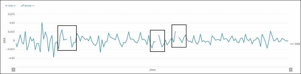
The preceding screenshot shows the output of the search result on the Splunk web console under the Visualization tab. The following screenshot shows the output of the same result under the Statistics tab:

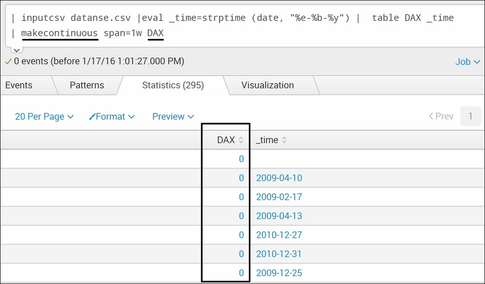
The preceding example output graph shows how there are breaks in the line chart when there is non-continuous data. So, the makecontinuous command adds empty bins for the period when no data is available, thus making the graph continuous. The second tabular image shows the time field along with the DAX field, which is specified to be made continuous and has values of 0. The span parameter is set to one week (1w), which is basically the size/range of the bin created to make the data continuous.

The Splunk addtotals command is used to compute the total of all the numeric fields or of the specified numeric fields for all the events in the result. The total value of numeric fields can either be calculated for all the rows, for all the columns, or for both of all the events.

The syntax for the addtotals command is as follows:

… | addtotals
    row=true / false
    col=true / false
    labelfield=Field_name
    label=Label_name
    fieldname=Fieldnames/ Field_list

Refer to the following list for parameter description about the options of the addtotals command:

Take a look at the following example of the addtotals command:

|inputcsv datanse.csv | table EM EU | addtotals col=true

The output of the preceding query will be similar to the following screenshot:

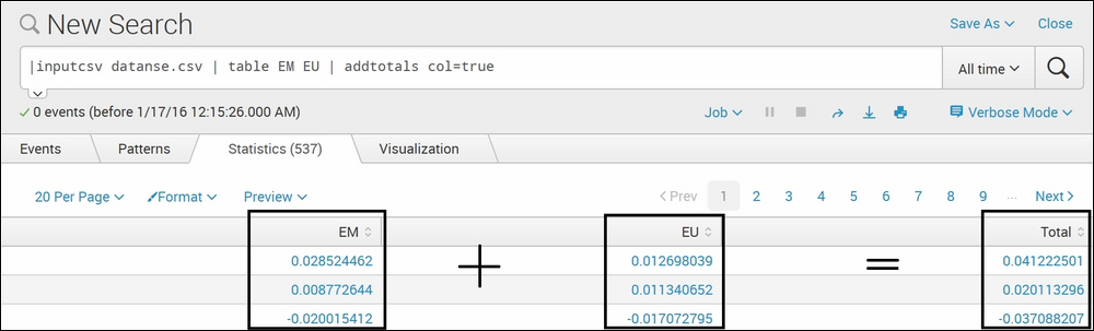
The Splunk addtotals command computed the arithmetic total of fields (EM and EU) and resulted in the fieldname Total. The parameter col is set to true, which means each column total is also calculated and resulted in the output.

The Splunk xyseries command is used to convert the data into a format that is Splunk visualization compatible. In other words, the data will be converted into a format such that the tabular data can be visualized using various visualization formats such as line chart, bar graph, area chart, pie chart, scatter chart, and so on. This command can be very useful in formatting the data to build visualizations of multiple data series.

Refer to the following query block for the syntax:

xyseries
    grouped=true / false
    x_axis_fieldname
    y_axis_fieldname
    y_axis_data_fieldname

The description of the parameters of the preceding query is as follows:

Refer to the following example for better clarity:

|inputcsvabc.csv |stats sum(Hits) AS Hits by Date UserID Transaction | eval temp=Date+"##"+UserID| table temp Transaction Hits | xyseries temp, Transaction Hits | fillnull | rex field=temp "(?<Date>.*)##(?<UserID>.*)" | fields - temp | table Date, UserID *

The output of the preceding query would look similar to the following screenshot:

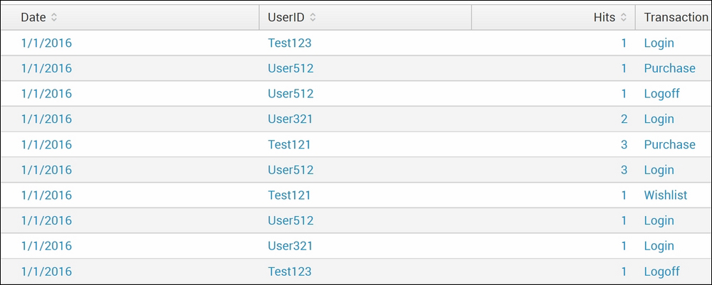
The preceding screenshot is the sample data image, which shows the data points on which we will run the xyseries command. The following screenshot shows the output of the search result on the given dataset:

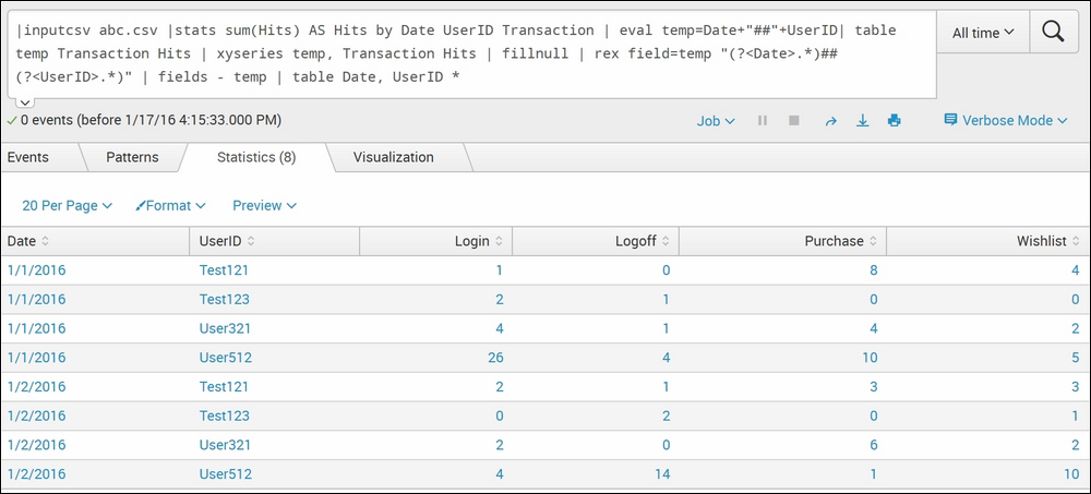
The first screenshot displays the data that is basically logging off the type of transaction and number of hits with respect to UserID and Time. In a scenario when the user wants a summary of, for example, all transactions done by each user on each date in the dataset, then the xyseries command can be used. In the example of xyseries, first, the stats command is used to create a statistical output by calculating the sum of hits based on Date, UserID and Transaction. Then, a temporary variable temp is created using the eval command to add Date and UserID into a fieldname temp. The xyseries command of Splunk is used to create a statistical output, and then, the temporary variable temp is expanded into its original variables, that is, Date and UserID. Hence, you get the result as required (shown in the second screenshot). Thus, the xyseries command can be used to plot data visualization for multiple data series.