
27
CASE STUDIES ON CRYSTALLIZATION SCALE‐UP
Nandkishor K. Nere, Moiz Diwan, Ann M. Czyzewski, James C. Marek, and Kushal Sinha
Process Research and Development, AbbVie Inc., North Chicago, IL, USA
Huayu Li
Material and Analytical Sciences, Boehringer Ingelheim Pharmaceuticals, Inc., Ridgefield, CT, USA
27.1 INTRODUCTION
Reliable scale‐up of crystallization processes requires a fundamental understanding of mixing and its impact on desired process performance attributes. The term “mixing” encompasses all aspects of hydrodynamics that dictate heat and mass transfer along with phase dispersion characteristics. In turn, hydrodynamics is governed by several equipment and process considerations, namely, (i) crystallizer geometry (size, aspect ratio), (ii) internals geometry/configuration (e.g. impeller type, size, location, number, and clearance; baffle type, size, location, and number; pump type, piping/tubing geometry, rotor–stator geometry, and configurations as applicable), (iii) physicochemical properties of fluid and solids, and (iv) operating parameters (speed of impeller, pump, and rotor–stator; fill level; feed rate/location; flow rates). Understanding and controlling hydrodynamics is a key to enabling robust process design and scale‐up; for further detailed characterization of hydrodynamics, the reader is referred to Ranade [1]. The key governing parameter characterizing the hydrodynamics of a system is the turbulent kinetic energy dissipation rate, which is defined as the rate of turbulent kinetic energy loss due to viscous forces in turbulent flow. The turbulent kinetic energy dissipation rate exhibits spatiotemporal heterogeneity. As depicted in Figure 27.1, the turbulent kinetic energy dissipation rate determines the kinetics of various underlying processes (i.e. heat and mass transfer, breakage/agglomeration, phase dispersions, etc.).
FIGURE 27.1 Scale‐up triangle showing energy dissipation rate controlling various key attributes for reliable scale‐up of crystallization processes.
In the case of crystallization processes, reliable scale‐up is heavily dependent upon the reproducibility of both local and global mixing characteristics across laboratory to pilot to commercial scale. While cooling crystallization is governed by heat transfer (hence both local and global mixing), antisolvent and reactive crystallizations are most strongly influenced by local mixing and will be the focus of this discussion. The reader is referred to Chapter 24 for in‐depth discussion related to cooling crystallization. The four case studies showcased in this discussion highlight how a thorough understanding of hydrodynamics and fundamentally the energy dissipation rate that is reflected through the micromixing time considerations led to reliable scale‐up. The first case study demonstrates that shear imparted by the impeller across scales in a given process can play a key role in not only crystal breakage and attrition but also the extent of secondary nucleation, both of which can impact crystal size distribution (henceforth referred to as particle size distribution or PSD). The second case study details an antisolvent crystallization process designed to circumvent negative impact of variability in local mixing intensities in a large batch vessel by instituting a high‐shear device outside the vessel in a recirculation loop. The third case study elaborates on the added complexity introduced when using an external mixing element in a crystallization process, namely, the need to characterize the evolution of the solvent composition of streams both in the crystallizer and in the recirculation loop. The final case study highlights the approach used to scale‐up a fed‐batch reactive crystallization in such a way to deliver product with consistent particle morphology. Taken together, these case studies demonstrate that fundamental understanding of mixing and associated considerations is imperative to developing scalable and robust crystallization processes.
27.2 CASE STUDY I: DESIGNING SHEAR EXPOSURE TO ACHIEVE SIMILAR BREAKAGE/ATTRITION ACROSS SCALES
27.2.1 Background
The example described in this section demonstrates a case in which careful design to control shear exposure had significant impact on improving particle physical properties. During laboratory‐scale development, a cooling crystallization process consistently delivered drug substance (DS) containing a significant amount of fines. Experiments were typically run at the 50 g scale in a 1L jacketed vessel with overhead stirring. Upon scale‐up to 50 gal pilot‐scale equipment, the crystallized product contained a significantly reduced amount of fines compared to laboratory batches. Scanning electron micrograph (SEM) images of the particles from both the lab scale and pilot scale demonstrate increased presence of fines in lab‐scale batches as evidenced by the increased number of fine particles observed on the surfaces of larger crystals in Figure 27.2a compared with Figure 27.2b).
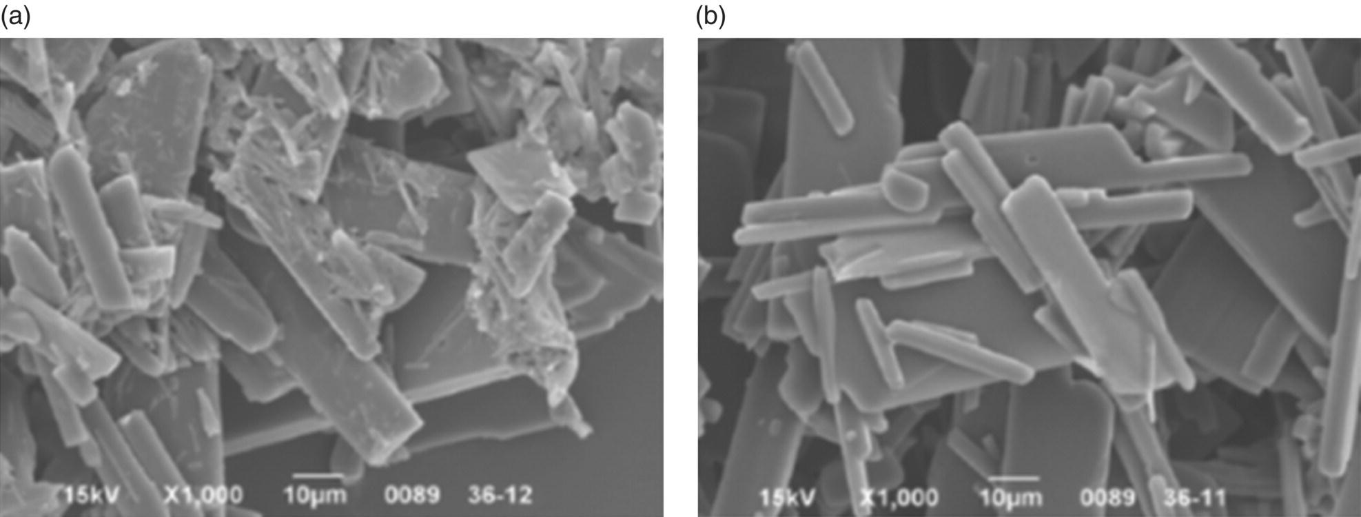
FIGURE 27.2 SEM images of crystals made from (a) lab‐scale cooling crystallization and (b) pilot‐scale cooling crystallization.
Smaller particle size crystals tend to cause slower and more operationally challenging isolations and can also negatively impact drug product processing. Therefore, ensuring control of the fines generated upon further scale‐up would ensure a more robust process, and efforts were directed at understanding and mitigating the root cause of their formation. The parabolic cooling profile employed at a supersaturation ratio (SSR) of 1.2 showed little to no evidence of causing secondary nucleation. Therefore, it was hypothesized that fines were caused primarily due to the energy input into the process via mixing. Further efforts were made to understand what aspects of the mixing may be impacting particle secondary nucleation and attrition.
27.2.2 Mixing Characterization
Breakage and attrition of crystals is primarily governed by the frequency of particle–particle, particle–wall, and particle–impeller collision as well as intensity of the impact. Both the frequency and intensity of collisions are dictated by local shear and the global convective flow pattern. The impeller region typically exhibits an order of magnitude higher shear rate compared with the global average shear. The shear imposed is directly related to the power input per unit volume, where the power is calculated as a volumetric integration of the turbulent energy dissipation rate (ε) as shown in Eq. (27.1):

where
- ρ is the average fluid/dispersion density.
In addition to the maximum shear, the cumulative time the crystallizer contents are passing through the impeller region also can impact particle physical properties. The average time particles spend passing through the impeller region can be quantified by calculating the number of turnovers (or number of passes, Npass) the slurry makes through the impeller region. A schematic depicting the direction of flow in and out of the impeller region of an agitated vessel is shown for reference in Figure 27.3.
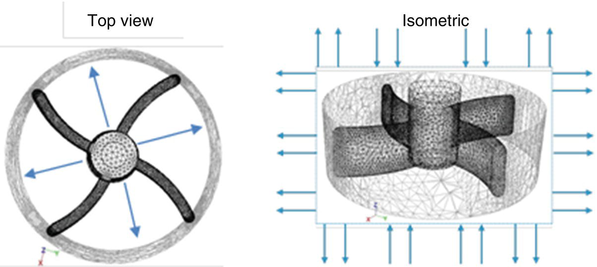
FIGURE 27.3 Top and isometric views of a rotating impeller and associated region. Arrows indicate the typical direction of fluid flow for radial flow impeller.
The number of passes through the impeller zone can be readily assessed based on parameters gleaned through computational fluid dynamics (CFD) simulations. The primary flow number (Nqd) represents the pumping capacity of the impeller and is calculated by determining the fluid flux out of the impeller region [2]. The primary flow number can be expressed as a function of the impeller speed (N), impeller diameter (D), and the radial or axial fluid velocity out of the impeller (vr or vz) as shown in Eqs. (27.2a) and (27.2b) for radial and axial flow impellers, respectively:
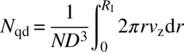

where
- RI and h are radius of the impeller for axial flow impeller and height of the blade for radial flow impeller.
The number of passes through the impeller zone (Npass) can then be calculated as a function of the flow number, impeller diameter, agitation speed, and operating solution/slurry volume (V) as shown in Eq. (27.3):
27.2.3 Results and Discussion
To understand the impact of mixing on the generation of fines, an analysis of the mixing from both the 50 g (1 L volume) and 10 kg (50 gal volume) DS crystallization processes was performed and is summarized in Table 27.1. It is notable in this example that neither the change in impeller tip speed nor the power per unit volume is consistent with the observation that a significantly greater number of fine particles were observed at the 1 L scale compared with the 50 gal scale. Looking at the number of passes through the impeller zone, however, it is clear that particles in the 1 L equipment experience higher cumulative exposure to shear, with a more than 7 times increase in the number of passes through the impeller zone compared with the same process run at the 50 gal scale. This significant increase in exposure of a crystallization mixture to the high‐shear mixing zone of the vessel can result in a greater extent of secondary nucleation as well as particle attrition, both of which contribute to more fine particles being observed in the product.
TABLE 27.1 Comparison for Mixing Characteristics in 1 L and 50 Gal Equipment
| 1 L Vessel (200 rpm) |
50 Gal Vessel (90 rpm) |
|
| Impeller tip speed (m/s) | 0.70 | 1.38 |
| Power per unit volume relative to 250 ml vessel (W/m3) | 1.05 | 0.95 |
| Passes through impeller zone (Npass, 1/h) | 1072 | 142 |
The results of CFD modeling of a more extreme change in scale for the same crystallization process are summarized in Table 27.2. Here, the mixing characteristics of a 250 ml laboratory‐scale vessel with a retreat curve agitator are compared with those of a 500 gal vessel equipped with a curved blade turbine impeller, similar to that shown in Figure 27.3. In this case, agitation speeds of the laboratory‐scale vessel (250 rpm) and the plant scale (40 rpm) were selected to deliver equivalent power per unit volume (5.8 W/m3).
TABLE 27.2 Comparison for Mixing Characteristics in 250 ml and 500 Gal Equipment
| 250 ml Vessel (250 rpm) | 500 Gal Vessel (40 rpm) | |
| Impeller tip speed (m/s) | 0.62 | 1.40 |
| Power per unit volume relative to 250 ml vessel (W/m3) | 1.08 | 1.0 |
| Passes through impeller zone (Npass, 1/h) | 1384 | 146 |
These data show that although power per unit volume is a commonly used parameter to scale‐up mixing, it may not be the only (or the most important) parameter that can significantly impact crystallization product particle size and shape distributions. In this example, while power per unit volume is relatively consistent across scales, the number of passes through the impeller zone is almost an order of magnitude greater in the 250 ml laboratory‐scale vessel compared with the 500 gal plant scale.
Since many factors can impact the success of a process scale‐up, it is important to reflect on multiple aspects of the hydrodynamic behavior that can impact product physical properties. The maximum shear imparted (reflected in the tip speed or power per unit volume) as well as cumulative shear exposure (quantified by the number of passes through the impeller zone) can both have significant impact on process outcomes in different situations. In this example, when the observed particle properties were not consistent with scale‐up based on maximum shear, deeper insight into additional contributing factors provided a context in which to understand the scale‐up outcome. In general, it is recommended that when scaling up a process for the first time, due consideration be given to potential impact of hydrodynamics in terms of both maximum and cumulative shear exposure in order to ensure robust process design.
27.3 CASE STUDY II: TAILORING MIXING TO ACHIEVE DESIRED CRYSTAL FORM AND PARTICLE SIZE DISTRIBUTION
The second case study describes a more complex crystallization process wherein control and proper scale‐up of mixing is required to achieve the desired DS crystal form in addition to appropriate physical properties. In this section, the complexity of the polymorph landscape coupled with the miscibility boundary of the ternary crystallization solvent mixture is described. The impact of mixing on the ability to deliver a product with a reproducible and scalable PSD is also discussed. Lastly, the process used to deliver quality product within both of these process design constraints is described followed by a summary of observed process performance across scales.
27.3.1 Polymorph Landscape and Basic Process Design
There are two polymorphs of the DS relevant to this case study: Form II is the desired thermodynamically stable form, and Form III is the undesired metastable crystal form. These polymorphs have distinct morphologies as shown by the polarized light microscopy (PLM) images shown in Figure 27.4.

FIGURE 27.4 Polarized light microscope images of (a) Form II and (b) Form III drug substance.
The ternary crystallization solvent system consisting of isopropyl acetate (IPAC), water, and isopropyl alcohol (IPA) was designed to deliver the desired Form II of the DS. Form competition and solubility studies (discussed in detail in Chapter 18) were used to establish understanding of the polymorph landscape and to construct the ternary phase diagram shown in Figure 27.5.

FIGURE 27.5 Ternary phase diagram (mass fraction) summarizing the thermodynamically stable crystal form at various solvent compositions relevant to the drug substance crystallization.
The circles in the phase diagram represent the solvent compositions where Form II is thermodynamically stable, and the corresponding space is marked by the dashed line on the plot. Outside of this region, particularly in IPA‐rich conditions, there is likelihood of crystallizing the undesired Form III, as indicated by the squares. The triangular markers demarcate the immiscibility boundary within which two liquid phases exist, both with and without the presence of DS.
Figure 27.6 is an alternative representation of the solvent composition space in which the water content and IPA content are normalized by the IPAC content, resulting in a two‐dimensional plot of solvent ratios (IPA/IPAC vs. water/IPAC). The solvent composition design space is enclosed within the dash‐dot boundary, and the immiscibility envelope is defined by the solid line/triangular markers. As described below, a dual‐addition crystallization was designed so that at any point during the addition, the solvent composition is maintained within a range that ensures the generation of only the thermodynamically stable Form II.

FIGURE 27.6 Two‐dimensional representation of the ternary phase diagram expressed as mass ratios of IPA/IPAC and water/IPAC.
The DS is introduced into the crystallization process as a solution in IPAC. To avoid traversing through solvent compositions within a Form III stable region of the phase diagram, the DS solution in IPAC and a premixed antisolvent mixture of IPA/H2O are added simultaneously (and at a specific ratio of addition rates) to a premixed IPAC/IPA/H2O solution in the crystallization vessel. This design, schematically represented in Figure 27.7, ensures that the entire crystallization is performed within solvent compositions in which Form II is thermodynamically stable, making the process robust for delivering the required crystal form of the DS. The modus operandi in which this basic process design was enhanced to ensure delivery of appropriate physical properties at pilot and commercial scale is discussed in the following section.
FIGURE 27.7 Schematic representation of dual‐addition antisolvent crystallization.
27.3.2 Control of Physical Properties
Because the formulation relevant to this case study is based on hot melt extrusion technology, tight control of the DS PSD is required to ensure successful drug product processing. Specifically, the formulation was found to be sensitive to the presence of agglomerates in the DS, due to the need to control residual DS crystallinity in the amorphous solid dispersion (ASD) dosage form. Following is a description on how the impact of mixing within the DS crystallization process was studied and controlled to ensure reproducible DS physical properties from pilot to commercial scale.
In the absence of a reliable method to assess intrinsic kinetics of fast crystallizations, an assessment of the relative kinetics at different mixing intensities (i.e. at different agitation speeds) was performed. While holding constant rate and location (relative to the impeller) of antisolvent addition, the observed counts per second measured by Lasentec FBRM were found to decrease with increased agitation speeds. This result suggests that the intrinsic crystallization kinetics is fast and that the overall kinetics of crystallization is mixing controlled. Therefore, local mixing must be maintained across scales to have similar overall crystallization kinetics.
Furthermore, the degree of mixing at the point in which the feed streams are added to the crystallizer was found to have significant impact on the physical properties of the crystallized DS. Adding both streams near a retreat curve agitator inside the crystallizer resulted in DS composed of loosely held agglomerated particles, as depicted in Figure 27.8. Due to the rapid nucleation and growth kinetics (compared to the micromixing time), the size of agglomerates generated was dependent on mixing efficiency during product solution addition. Once the agglomerates were formed, breaking them using dry milling or high‐shear rotor–stator (wet milling) technologies resulted in a bimodal PSD due to variability in agglomerate strength. The bimodal PSD presented two undesirable attributes. The agglomerates promoted residual crystallinity in the drug product, and the material exhibited poor flow properties, which negatively impacted manufacturability of the downstream drug product manufacturing process.
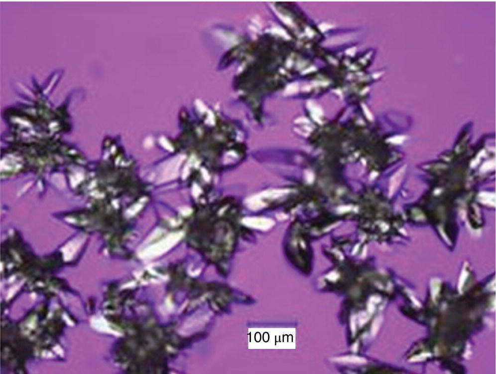
FIGURE 27.8 Polarized light microscopy image of agglomerated Form II particles crystallized from the dual addition of feed streams into the crystallizer.
Based on these observations, higher intensity, more consistently controlled mixing during crystallization was required across various scales to ensure suitable control of DS physical properties. Options for enhancing mixing outside of the crystallizer were considered. Typical mixing time within a recirculation loop, for example, with an assumed flow rate of 140 L/min and 1.5 in diameter tube (flow velocity of ~2 m/s) is on the order of 50 ms. This mixing may be slightly better compared with the mixing time obtained near the agitator of the stirred tank, but still would not be sufficient to minimize particle agglomeration.
To overcome mixing limitations at the point of addition of the DS feed stream, a high‐shear rotor–stator mixer (wet mill) was incorporated into the process, wherein the micromixing time inside the rotating elements is estimated to be less than 10 ms. The high‐shear mixer is composed of three rotor–stator pairs in series that interact with the fluid. As shown in the process flow diagram in Figure 27.9, the DS feed solution is added into a recirculation stream, followed immediately by passage of this stream through a high‐shear mixer. Ensuring the micromixing time (<10 ms) is sufficient results in DS that is predominantly primary particles, as shown by the PLM image depicted in Figure 27.10. Using the high‐shear mixer minimizes the local buildup of high supersaturation and results in a process that is independent of the design of the crystallizer while achieving consistent mixing across scales of interest.
FIGURE 27.9 Drug substance crystallization process flow diagram using high‐shear rotor–stator‐based mixing in the recirculation loop.

FIGURE 27.10 PLM image of Form II particles crystallized using high‐shear rotor–stator‐based mixing
The complete, final design of the DS crystallization process is shown schematically in Figure 27.9. As depicted in the process flow diagram, vessel 1 contains the DS solution in IPAC, and vessel 2 holds the IPA/water antisolvent mixture. A mixture of IPAC/IPA/water is prepared in the crystallizer. The next step is to generate a saturated DS solution that will sustain the charge of seed crystals. The saturated solution is created by simultaneously adding a portion of the vessel 1 solution to the tee at the inlet of the high‐shear rotor–stator mixer and a portion of the vessel 2 solution to the crystallizer at a fixed addition rate ratio (antisolvent to DS solution). Once the solution is saturated, DS Form II seeds are charged. The slurry is then circulated through the high‐speed rotor–stator‐based mixer with the simultaneous addition of a portion of vessel 1 contents and a portion of the vessel 2 contents at a fixed addition rate ratio to crystallize the product.
It is important that the ratio of the recirculation rate to the product solution addition rate is held constant during crystallization. At a given recirculation rate through high‐shear mixer, slow batch addition affords good mixing of the added streams and produces predominantly primary particles. However, a study done with fast batch addition during crystallization resulted in loosely held agglomerates (due to locally high supersaturation), which broke to a greater extent upon filtration and drying and led to a bimodal PSD.
The impact of using a high‐shear mixer as described on the DS PSD was investigated. As shown in Figure 27.11, using a conventional process (adding the DS solution inside the reactor) resulted in a broad PSD compared with the narrower distribution obtained using the high‐shear mixer.

FIGURE 27.11 Comparison of particle size distribution measured by laser diffraction analysis (Malvern®) from conventional mixing (dashed lined) and high‐shear rotor–stator‐based mixing (continuous line).
A summary of the PSD of various batches of DS made throughout the development and into commercial production is shown in Table 27.3. It is notable that the variability in PSD observed in the early pilot plant batches made without the use of the high‐shear mixer was greatly mitigated in the final crystallization process. Implementation of the high‐shear mixer delivered product of consistent particle size at both the pilot plant and commercial scales. Moreover, these data demonstrate that the PSD can be tuned by adjusting the high‐shear mixer parameters (rotor–stator configuration, recirculation rate, and rotor tip speed) to enable optimal performance in the drug product process.
TABLE 27.3 Particle Size Distribution Results Using Various Mixing Configurations
| Mixing Configuration | Lot ID | PSD (μm) | ||
| d10 | d50 | d90 | ||
| Conventional mixing Non‐reproducible PSD with traditional process |
Early Pilot Plant Lot 1 | 78 | 184 | 339 |
| Early Pilot Plant Lot 2 | 22 | 66 | 144 | |
| High‐shear rotor–stator‐based mixing in recirculation loop Consistent performance of the manufacturing process at scale using optimized mixing Ease of process transfer to commercial plant |
Pilot Plant Lot 1 | 20 | 64 | 143 |
| Pilot Plant Lot 2 | 28 | 67 | 133 | |
| Pilot Plant Lot 3 | 13 | 54 | 145 | |
| Commercial Lot 1 | 11 | 48 | 158 | |
| Commercial Lot 2 | 13 | 52 | 141 | |
| Commercial Lot 3 | 11 | 46 | 159 | |
| High‐shear mixer parameter studies Ability to tune particle size distribution (PSD) by varying process parameters for optimal drug product performance |
Very small particles | 7 | 17 | 52 |
| Large predominately primary particles | 15 | 54 | 148 | |
| Large agglomerated particles | 61 | 165 | 296 | |
27.4 CASE STUDY III: SCALE‐UP CONSIDERATIONS FOR ANTISOLVENT ADDITION INTO A RECIRCULATION LOOP
As was demonstrated in the previous case study, intense and consistent mixing is achieved by addition of antisolvent into a high shear zone. Consistent and sufficient mixing can in some cases be alternatively accessed in the impeller region of the crystallizer and/or within a recirculation loop (high velocity addition into tubing/piping or into the impeller eye of the centrifugal pump). To ensure development of a robust crystallization process, mixing in these areas needs to be appropriately scaled. Higher flow velocities naturally provide a viable means of achieving better mixing; however flow velocity cannot be increased arbitrarily without considering the relevant residence time. The ratio of the average residence time (calculated by dividing the operating volume by the recirculation flow rate) to the mixing/blend time of at the least 10 is expected to approximate a well‐mixed batch vessel (akin to the analogy of ideal CSTR behavior requirements; see Chapter 13). For practical purposes it is recommended to maintain a ratio significantly higher than 10; as the scale of crystallizer operating volume increases, more heterogeneity in the mixing is expected.
An additional consideration in the design of antisolvent crystallizations is that the solvent composition and solute concentration (and thus supersaturation) changes as a function of time. Therefore, in the design of a process in which antisolvent is added into a recirculation loop, it is important to ensure that the evolution of solvent composition and solute concentration in both the crystallizer and recirculation loop is consistent across scales. In this way, the rate of antisolvent addition and recirculation flow rate need to be chosen not only to deliver appropriate mixing characteristics but also to achieve similar temporal profiles of solvent composition and solute concentration in both the recirculation loop and the main crystallizer across various scales of operation. The following theoretical example focuses on the due considerations around these aspects.
27.4.1 Theoretical Analysis of Antisolvent Crystallization Added in the Recirculation Loop
Figure 27.12 depicts a schematic of an antisolvent crystallization configuration in which the antisolvent (solvent B) is added into the high‐shear region of the recirculation loop. The main crystallizer contains a co‐solvent (solvent A) and also contains the solute to be crystallized totaling a mass, MT. The concentration of each solvent in the loop (SA,loop and SB,loop) and solute in the loop (Ss,loop) and the corresponding concentrations in the tank (SA,T, SB,T, and SS,T) are functions of time, as shown. The flow rates into and out of the vessel are shown as ![]() and
and ![]() , respectively, and the antisolvent addition flow rate into the addition tee is designated as
, respectively, and the antisolvent addition flow rate into the addition tee is designated as ![]() . The total holdup in the recirculation loop (RT) consists of the holdup in the lines before the antisolvent addition (RB) and after the antisolvent addition (RA) and holdup in the process equipment (high‐shear mixer and the pump, Reqmt).
. The total holdup in the recirculation loop (RT) consists of the holdup in the lines before the antisolvent addition (RB) and after the antisolvent addition (RA) and holdup in the process equipment (high‐shear mixer and the pump, Reqmt).
FIGURE 27.12 Schematic of the recirculation loop along with the stream compositions of solvents and solute.
The objective of this type of evaluation is to understand how different the solute and solvent concentration profiles in the tank are from the respective concentrations in the recirculation loop over the course of the antisolvent addition. Any observed difference can then be assessed in the context of its impact on supersaturation and hence on the crystallization process. This evaluation begins with establishing the material balance as the basis for the calculations.
Concentrations of solvent A and solute S in the crystallizer change over time due to the dilution effect caused by the addition of antisolvent B. For example, the total solute concentration can readily be calculated from the Eq. (27.4), and a similar equation could be written for solvent A:

However, concentration profile of the antisolvent B in the crystallizer can be obtained by solving the following ordinary differential equation using Matlab® or Polymath® software with the known initial conditions of the total mass in the tank [MT(0)], the antisolvent mass fraction [SB, T(0) = 0], and the total mass hold in the loop for a given mass flow rate of the antisolvent, ![]() :
:
where
- RT = RA + RB + Reqmt is the total holdup volume in the recirculation loop and associated equipment.
Furthermore, based on simple mass balance around the point of addition of antisolvent in the recirculation loop, one can easily infer the concentrations of solvents and solute in the loop. For example, the concentration of solvent A in the loop would be given by

For this theoretical case study, application of the analysis described above is demonstrated in the context of a simple antisolvent addition crystallization process. The crystallization process is designed such that initially, the solute is dissolved in 0.19 kg solute/kg solution in the solvent A. Antisolvent (solvent B, 9.6 kg/kg of solute) is then added into a recirculation loop over a period of three hours to complete the crystallization. Two batch configurations are considered, including a 25 kg nominal batch size and a 175 kg batch size, representing a 7× scale‐up of the process. Relevant parameters and initial conditions for two such batches are summarized in Table 27.4.
TABLE 27.4 Process Parameters and Initial Conditions for a 25 and 175 kg Batch Size Antisolvent Addition Crystallization Process
| Batch Size (kg) | Initial Mass in the Crystallizer, MT(0), (kg) | Mass Fraction of Solvent, SA, T(0) kg Solvent/kg Solution | Mass Flow Rate of Antisolvent, |
Recirculation Flow Rate (kg/min) | Antisolvent Added (kg) | Time of Antisolvent Addition (h) |
| 25 | 137.5 | 0.81 | 1.14 | 33.14 | 240 | 3 |
| 175 | 962.5 | 0.81 | 7.98 | 115.99 | 1678 | 3 |
TABLE 27.5 Supersaturation Ratios (![]() ) and Seed Loading Used for Spike Experiments
) and Seed Loading Used for Spike Experiments
| Spike Number | SSR | Seed Concentration (mg/g) |
| 1 | 7.6 | 1.28 |
| 2 | 4.2 | 0.19 |
| 3 | 4.2 | 0 |
The temporal evolution of the ratio of solvent B (process antisolvent) to solvent A (process solvent) in both the crystallizer and the recirculation loop is shown in Figure 27.13a for the 25 kg batch size and Figure 27.13b for the 175 kg batch size. Notably, the ratio of antisolvent in the crystallizer and in the recirculation loop diverges from each other in both cases, and the difference becomes more pronounced at increased batch scales. Moreover, the difference in solvent ratio in the crystallizer and the recirculation loop grows over time in both cases, with the recirculation loop being enriched in antisolvent. While it may appear at first glance that these differences in crystallizer/recirculation loop solvent ratios over time and across scales are relatively minor, such a change may have significant impact on supersaturation, depending on the slope of the solubility curve and on the rate of crystallization kinetics. Hence, the systems that have the fastest crystallization kinetics and steepest solubility curves are expected to have the greatest impact on supersaturation. In such a case, one may anticipate the potential for a divergence in physical properties of crystals nucleated and/or grown in the crystallizer compared with the recycle loop over time.
FIGURE 27.13 Ratio of solvent B (antisolvent) to solvent A (solvent) in the crystallizer and the recirculation loop over the course of a three hour antisolvent addition for the process described in Table 27.4 at (a) 25 kg scale and (b) 175 kg scale.
By a similar analysis, the ratio of antisolvent (solvent B) to total solute was profiled over time for batches at both the 25 and 175 kg scales, as shown in Figure 27.14a and b, respectively. A similar trend is observed in this data, with a notable divergence between the crystallizer and recirculation loop concentrations of antisolvent with increased scales.
FIGURE 27.14 Ratio of solvent B (antisolvent) to total solute in the crystallizer and the recirculation loop over the course of a three hour antisolvent addition for the process described in Table 27.4 at (a) 25 kg scale and (b) 175 kg scale.
Figure 27.15 displays a profile of how the total solute concentration in both the crystallizer and recirculation loop evolves over the course of the antisolvent addition at both the 25 and 175 kg scales. The total solute concentration in the crystallizer is slightly higher than that in the recirculation loop, driving supersaturation higher in the crystallizer compared with the recirculation loop.
FIGURE 27.15 Total solute concentration in the crystallizer and the recirculation loop over the course of a three hour antisolvent addition for the process described in Table 27.4 at (a) 25 kg scale and (b) 175 kg scale.
This analysis shows that these highly interrelated measures of solvent ratios and solute concentration can impact the SSR differently in different parts of the reactor configuration. It should also be noted that these differences may get amplified in the systems involving more than two solvents, and it is therefore recommended to carry out similar analyses to inform appropriate scale‐up considerations.
27.4.2 Summary Considerations
The case study shown here elaborates possible concerns that need to be addressed for designing the scale‐up of the process involving the use of a recirculation loop meant to enhance mixing. While local mixing can be managed well in such a process design, it is also important to keep the crystallization trajectories the same in both the recirculation loop and the crystallizer to yield similar process performance. In order to ensure similar performance, it is necessary to either use recirculation equipment with appropriate capacities or limit the scale‐up to a smaller batch size to achieve similar crystallization performance across various scales. In practice, the high‐shear mixer and associated pump are available in discrete capacities (e.g. 10 GPM and 35 GPM IKA® high‐shear mixers) and do not necessarily provide appropriately scaled‐up flow rates at various batch sizes that may be of interest. Therefore, it is necessary to be cognizant of inherent scale‐up limitations due to available or limited process equipment capacities. If the equipment available for scale‐up has sufficiently large capacity, then the maximum recirculation rate should be capped by the desired maximum ratio of the mean residence time to mixing time in the crystallizer.
Due consideration must also be given to the residence time in the high‐shear mixer, which could be an important scale‐up criterion, as discussed in the first case study of this chapter. For example, if scale‐up of “breakage” in a high shear zone that occurs concurrent to antisolvent addition is important, then maintaining a consistent number of turnovers can only be achieved if the residence time in the high‐shear mixer is kept constant. Higher flow rates required to achieve good mixing may result in a lower residence time and hence may require an increased number of turnovers through the high‐shear mixer upon scale‐up.
27.5 CASE STUDY IV: MORPHOLOGY CONTROL IN A REACTIVE CRYSTALLIZATION
Fed‐batch reactive crystallizations are inherently complex in that there exists a complex interplay between the rate of reaction, kinetics of crystallization, and mixing, which in turn may impact the physical properties of the resultant product. This fourth case study describes the approach used to understand both the rate of reaction and crystallization kinetics in order to scale‐up a fed‐batch reactive crystallization process that delivers consistent DS physical properties.
27.5.1 Introduction
The process flow diagram of a reactive crystallization used to manufacture the DS of interest in this case study is shown in Figure 27.16a. The monohydrochloride salt of the DS is charged into a basic sodium carbonate (1.4 equiv.) solution at the desired pH. A seed slurry in isopropanol (IPA)/water is added to ensure control of the desired crystal form. The monohydrochloride salt immediately reacts with the base, resulting in the generation of supersaturation followed by the crystallization of DS free base.

FIGURE 27.16 (a) Crystallization process flow diagram. (b) Schematic depicting impact of mixing on reaction/crystallization at the point of addition of DS solution into the basic solution.
Figure 27.16b is a schematic that depicts the complex processes involved at the location where the DS solution contacts the base. It is at this point where both reaction and crystallization are occurring, the relative rates of which, along with the intensity of mixing, impact the local supersaturation. As described in this case study, understanding these phenomena was important to establishing a control strategy to reproducibly deliver the desired product morphology.
27.5.2 Crystallization Kinetics
The solubility of the DS free base was measured as a function of base concentration and isopropanol content at 20 °C and is summarized in Figure 27.17. The solubility decreases with increasing sodium carbonate content but is very low, ranging from 1.2 to <0.1 mg/g, throughout the range studied. Moreover, the isopropanol introduced through the seed slurry into the crystallization process does not impact the DS solubility significantly. This low solubility in the crystallization solvent system results in inherently high supersaturation of the DS free base at the point of contact between the hydrochloride salt and basic crystallization medium due to fast reaction.
FIGURE 27.17 Solubility of the DS free base as a function of sodium carbonate concentration and isopropanol content at 20 °C.
A very rapid nucleation of crystals observed under nominal processing conditions is not suitable for interrogating crystallization kinetics due to the inability to sample and monitor the process over time. White solids were observed to precipitate upon the dropwise addition of the DS HCl solution to sodium carbonate base under nominal processing conditions. The nominal condition is indicated by a large circle in the upper right corner in the plot of DS HCl concentration as a function of sodium carbonate concentration (Figure 27.18). Similar observations of rapid crystallization were noted at all conditions marked with open circles in Figure 27.18. At sufficiently lower base concentrations and/or DS HCl solution concentrations, phase separation was observed, followed by slow conversion to crystalline product. This behavior was observed at conditions marked with diamonds in Figure 27.18. The low base/low DS HCl concentration conditions (marked in the lower left corner of Figure 27.18) were selected as appropriate conditions for accessing crystallization kinetics.
FIGURE 27.18 Precipitation domain map as a function of sodium carbonate concentration and DS HCl salt concentration at 20 °C.
Three experiments were performed in which a supersaturation spike was generated to a desired level and the desupersaturation profile was monitored over time. All experiments were executed under the same agitation rate (400 rpm) and under conditions with the same thermodynamic solubility (1.16 mg/g at 20 °C). Table 27.5 lists SSR (denoted by S) along with the seed loading used for each of the spike experiments.
Desupersaturation profiles for each of these spike experiments are summarized in Figure 27.19.
FIGURE 27.19 Desupersaturation profile for crystallization kinetics studies.
These desupersaturation profiles were used in population balance modeling and parameter fitting to estimate the primary nucleation rate (B1), secondary nucleation rate (B2), and crystal growth rate (G). These parameters were modeled using the method of moments [3] and minimization of the sum of squared error (∑(csim − cexp)2) between experimental data and simulation results [4, 5]. Fitting results for the three spiking studies are shown in Figure 27.20.
FIGURE 27.20 Parameter fitting results from spiking experiments.
Equations for the primary nucleation rate, secondary nucleation rate, and growth rate are shown in Eqs. (27.7), (27.8), and (27.9), respectively. The exponent of 22.7 in Eq. (27.7) is significantly higher than the typical value of 3–4. A high value for this exponent suggests the process is dominated by primary nucleation [6]. It is likely, however, that variability in local supersaturation contributed to estimation of this extraordinarily high result. The apparent difference between the locally high supersaturation due to pockets of inhomogeneity at the point of nucleation (exacerbated by low solubility for a fast acid–base reactive crystallization), which is responsible for underlying crystallization, and the average (lower value) supersaturation used for parameter fitting might have resulted in overestimation of the primary nucleation rate exponent.
where
- ms is the mass of crystals:
The time scale (in minutes) for crystallization can be inferred from the crystallization (i.e. primary nucleation and growth) kinetics due to the change in concentration (Δc in g/g solvent) as per Eq. (27.10):
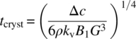
Using this relationship, crystallization time scales were calculated as a function of SSR and plotted in Figure 27.21. Over the SSR range of 5–50, the crystallization time varies from microseconds to seconds. In the event that this time scale of crystallization is similar to that of the micromixing time, it may be the case that the crystallization and mass transfer are competing phenomena. As discussed in the next section, insufficient mixing may allow DS free base to nucleate under locally high SSR.
FIGURE 27.21 Calculated time scale of crystallization as a function of supersaturation ratio.
27.5.3 Mixing Characterization
CFD simulations were performed to assess the hydrodynamics in the crystallizer and calculate the time scale of mixing. Both the micromixing time and mesomixing time (Figure 27.22a and b, respectively) were calculated throughout the fluid domain under operational conditions. While the micromixing time represents the time scale of mixing at diffusion length scales (Kolmogorov length scale), the mesomixing time is the time it takes to dissipate a feed stream into a batch by turbulent dispersion.

FIGURE 27.22 Contour plots of micromixing and mesomixing times calculated from CFD simulations in 500 L reaction vessel with the agitation speed of 100 rpm.
The mesomixing time at the liquid surface of the agitated vessel where the feed stream is introduced to the main batch during the DS mono HCl addition is of the order of hundreds of milliseconds. The relative rate of the mesomixing time compared with reaction/crystallization rate impacts physical properties of the resultant DS, as discussed in the following section.
27.5.4 Impact on Particle Morphology
As was discussed in case study II, in the absence of a reliable method to assess intrinsic kinetics of fast crystallizations, it can be informative to assess relative kinetics. In this case, experiments were performed to evaluate how variation in the reaction rate (modulated via the base concentration) and variation in the degree of mixing impact the particle morphology of the resultant product. Figure 27.23 shows scanning electron microscope (SEM) images of products obtained from (Figure 27.23a) the nominal base concentration, (Figure 27.23b) increase of the base concentration to 133% of nominal, and (Figure 27.23c) 50% of the nominal base concentration (reduced by half) while holding the mixing rate constant. At higher base concentration, the image in Figure 27.21b shows that the increased reaction rate resulted in agglomerated particles composed of fine primary particles. At reduced base concentration, the reduced reaction rate resulted in large primary particles with smooth surfaces (Figure 27.23c). The nominal base concentration resulted in a mixture of larger primary particles and fines (Figure 27.23a).

FIGURE 27.23 Scanning electron micrograph (SEM) images of products from crystallizations run at (a) nominal base concentration, (b) 133% nominal base concentration, and (c) 50% decrease from nominal base concentration while maintaining consistent agitation speed.
The ability to modulate the morphology by varying the base concentration is indicative of the crystallization being reaction rate limited. At reduced base concentrations, the slowed reaction rate leads to reduced DS free base concentrations and a low SSR, which leads to large primary particles with smooth crystal surfaces. On the other hand, increased base concentration leads to faster reaction rate and higher DS free base concentrations, resulting in a high SSR, causing rapid nucleation of fine particles, which agglomerate into irregular shapes. The nominal base concentration resulting in a mixture of both particle morphologies appears to be operating in conditions where the local supersaturation is in a transition region where both the nucleation and growth kinetics are prevalent.
The results from a similar experiment in which base concentration was held constant (nominal base concentration) and the agitation speed was varied from 50, 100, and 400 rpm are summarized in Figure 27.24. These images show that the morphology remained consistently a mixture of larger and fine primary particles agglomerated together across all agitation speeds tested. These results confirm that this crystallization is not mixing limited.
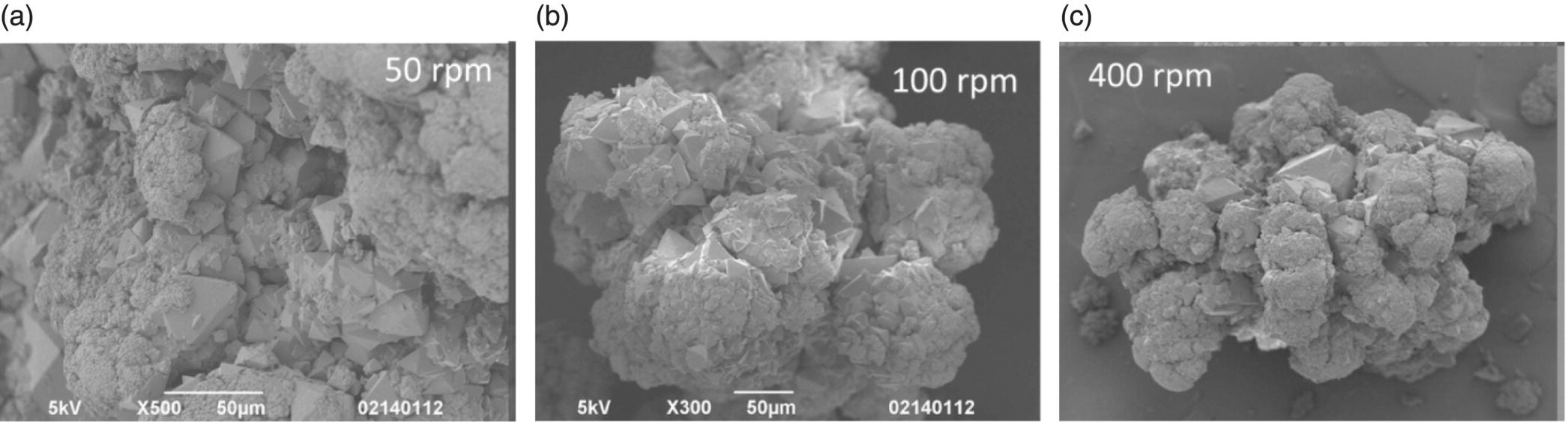
FIGURE 27.24 SEM images of products from crystallizations run at agitation rates of (a) 50 rpm, (b) 100 rpm, and (c) 400 rpm while maintaining nominal base concentration.
The understanding of how to modulate physical properties gained from this study was used to readily produce batches of DS with properties that varied over a broad range. In this case, the optimal particle morphology for downstream processing and formulation was the finer. Agglomerated particles were observed from the higher base concentrations. The process understanding was successfully scaled‐up by controlling the base addition (and thus the rate of reaction) and ensuring mixing was sufficient across all scales to maintain similar overall rates of reaction and hence the local supersaturations.
This case study demonstrates several of the complexities of characterizing and scaling up a reactive crystallization. Assessment of reaction, crystallization, and mixing using appropriately designed experiments is critical to fundamentally understanding key aspects of the process. These results should be then used as a basis for reliable scale‐up of reactive crystallization processes.
ACKNOWLEDGMENT
Authors would like to acknowledge experimental support from Rajarathnam Reddy and Alessandra Mattei and useful technical discussions and insights from Shailendra Bordawekar, Samrat Mukherjee, and Ahmad Sheikh.
REFERENCES
- 1. Ranade, V.V. (2002). Computational Flow Modelling for Chemical Reactor Engineering. New York: Academic Press.
- 2. Nere, N.K., Patwardhan, A.W., and Joshi, J.B. (2003). Liquid‐phase mixing in stirred vessels: turbulent flow regime. Industrial and Engineering Chemistry Research 42 (12): 2661–2698.
- 3. Randolph, A. (1988). Theory of Particulate Processes: Analysis and Techniques of Continuous Crystallization, 2e. San Diego, CA: Elsevier Inc.
- 4. Miller, S.M. and Rawlings, J.B. (1994). Model identification and control strategies for batch cooling crystallizers. AIChE Journal 40 (8): 1312–1327.
- 5. Togkalidou, T., Tung, H., Sun, Y. et al. (2004). Parameter estimation and optimization of a loosely bound aggregating pharmaceutical crystallization using in situ infrared and laser backscattering measurements. Industrial and Engineering Chemistry Research 43 (19): 6168–6181.
- 6. Aoun, M., Plasari, E., David, R., and Villermaux, J. (1999). A simultaneous determination of nucleation and growth rates from batch spontaneous precipitation. Chemical Engineering Science 54 (9): 1161–1180.