Motor Drives
Muhammed F. Rahman The University of New South Wales, Sydney, NSW, Australia
Dean Patterson University of Nebraska, Lincoln, LE, United States
Adrian Cheok Imagineering Institute, Nusajaya, Malaysia
Robert Betz University of Newcastle, Callaghan, NSW, Australia
Abstract
The widespread proliferation of power electronics and ancillary control circuits into motor control systems in the past several decades have led to a situation where motor drives, which process about two-thirds of the world's electric power into mechanical power, are on the threshold of processing all of this power via power electronics. The days of driving motors directly from the fixed ac or dc mains via mechanical adjustments are truly over. Table 30.1 indicates application areas where various types of power electronic converter-driven motor drives are routinely used.
Table 30.1
Typical motor, converter, and application guides
| Motor | Type of converter | Type of control | Applications |
| Brushed dc motor | Thyristor ac-dc converter | Phase control, with inner current loop | Process rolling mills, winders, locomotives, large cranes, extruders, and elevators |
| GTO/IGBT/MOSFET chopper | Pulse-width modulator (PWM) control with inner current loop | Drives for transportation, machine tools, and office equipment | |
| Induction motor (cage) | Back-back thyristor | Phase control | Pumps and compressors |
| IGBT/GTO inverter/cycloconverter | PWM V-f control | General-purpose industrial drive such as for cranes, pumps, fans, elevators, material transport and handling, extruders, and subway trains | |
| IGBT/GTO | Vector control | High-performance ac drives in transportation, motion control, and automation | |
| Induction motor (slip ring) | Thyristor ac-dc converter | Phase control with dc-link current loop | Large pumps, fans, and cement kilns |
| Synchronous motor (excited) | Thyristor ac-dc converter | DC-link current loop | Large pumps, fans, blowers, compressors, and rolling mills |
| Synchronous motor (PM) | IGBT/MOSFET inverter | PWM current control | High-performance ac servo drives for office equipment, machine tools, automotive traction drives and motion control |

Keywords:
DC motor drives; Induction motor drives; Synchronous motor drives; Switched reluctance motor drives; Stepping motor drives; Torque control; Inverter; Vector control; Synchronous reluctance motor drives
30.1 Introduction
The widespread proliferation of power electronics and ancillary control circuits into motor control systems in the past several decades have led to a situation where motor drives, which process about two-thirds of the world's electric power into mechanical power, are on the threshold of processing all of this power via power electronics. The days of driving motors directly from the fixed ac or dc mains via mechanical adjustments are truly over. Table 30.1 indicates application areas where various types of power electronic converter-driven motor drives are routinely used.
The widespread incorporation of power, control, and signal electronics in motor drives has meant that processes can now be driven much more efficiently with a much greater degree of flexibility than previously possible. Of course, certain processes are more favorable to certain types of motors, because of the more favorable match between their characteristics. Historically, this situation was brought about by the demands of the industry. Increasingly, however, power electronic devices and control hardware are easily tailoring the rigid characteristics of the motor (when driven from a fixed dc or ac supply source) to the requirements of the load. Development of novel forms of machines and control techniques therefore has not abated, as recent trends would indicate.
It should be expected that just as power electronics equipment has tremendous variety, depending on the power level of the application, motors also come in many different types, depending on the requirements of application and power level. Often, the choice of a motor and its power electronic drive circuit for application is forced by these realities, and the application engineer therefore needs to have a good understanding of the application, the available motor types, and the suitable power electronic converter and its control techniques. Table 30.1 gives a rough guide of combinations of suitable motors and power electronic converters for a few typical applications.
For many years, the brushed dc motor had been the natural choice for applications requiring high dynamic performance. Drives of up to several hundred kilowatts have used this type of motor. In contrast, the induction motor was considered for low-performance, adjustable-speed applications at low and medium power levels. At very high power levels, the slip-ring induction motor or the synchronous motor drive was the natural choice. These boundaries are increasingly becoming blurred, especially at the lower power levels, especially for AC motor drives.
Another factor for motor drives was the consideration for servo performance. The ever-increasing demand for greater productivity or throughput and higher quality of most of the industrial products that we use in our everyday lives means that all aspects of dynamic response and accuracy of motor drives have to be increased. Issues of energy efficiency and harmonic proliferation into the supply grid are also increasingly affecting the choices for motor-drive circuitry.
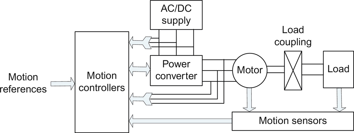
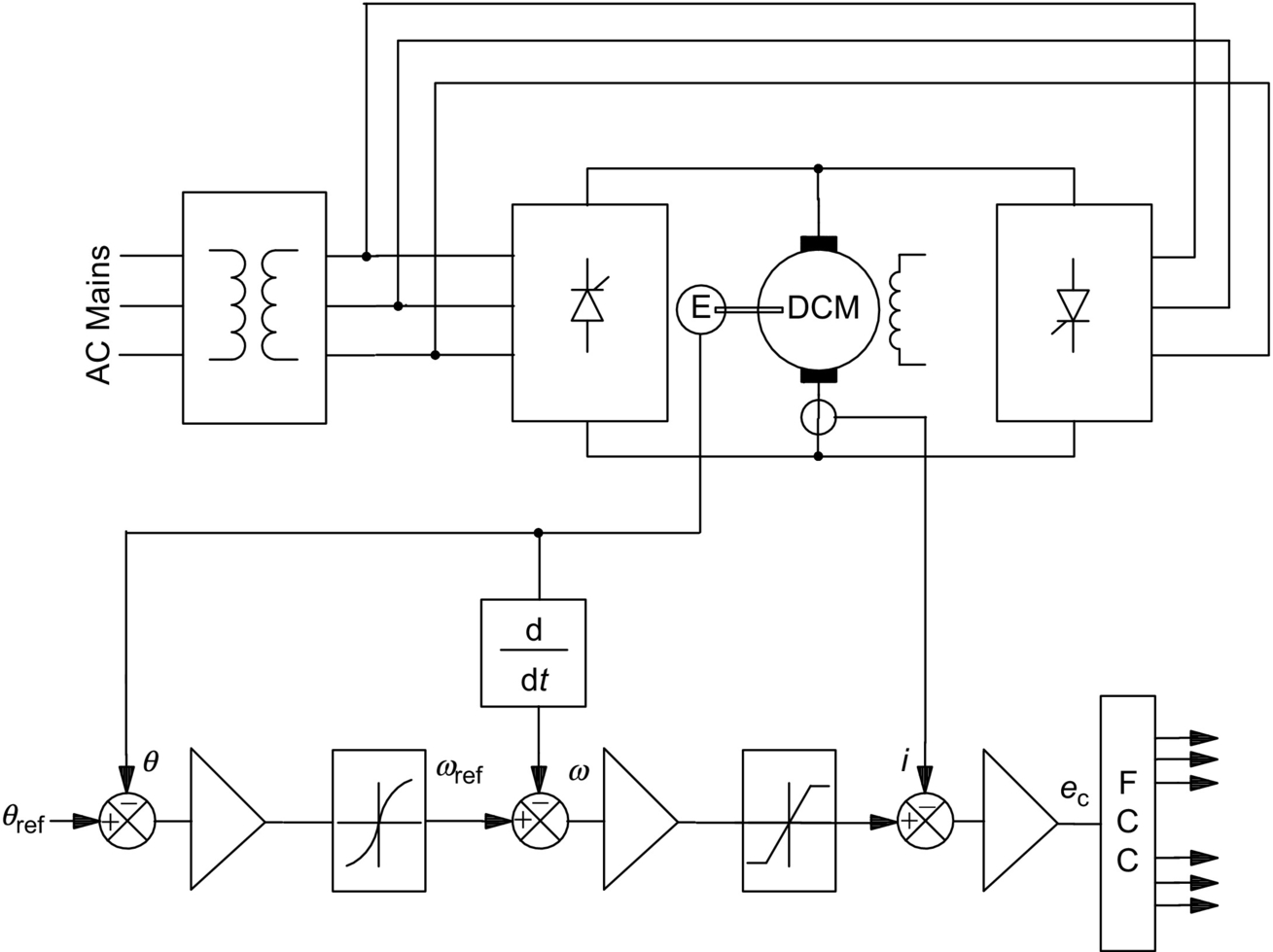
A typical motor-drive system is expected to have some of the system blocks indicated in Fig. 30.1. The load may be a conveyor system, a traction system, the rolls of a mill drive, the cutting tool of a numerically controlled machine tool, the compressor of an air conditioner, a ship propulsion system, a control valve for a boiler, a robotic arm, and so on. The power electronic converter block may use diodes, metal oxide semiconductor field-effect transistors (MOSFETS), gate turnoff thyristors (GTOs), insulated gate bipolar transistors (IGBTs), or thyristors. The controllers may consist of several control loops, for regulating voltage, current, torque, flux, speed, position, tension, or other desirable conditions of the load. Each of these may have their limiting features purposely placed in order to protect the motor, the converter, or the load. The input commands and the limiting values to these controllers would normally come from the supervisory control systems that produce the required references for a drive. This supervisory control system is normally more concerned with the overall operation of the process rather than the drive.
Consequently, a vast array of choices and technologies exist for a motor-drive application. Against this background, this chapter gives a brief description of the dominant forms of motor drives in current usage. The interested reader is expected to consult further reading material listed at the end of this chapter for more detailed coverage.
30.2 DC Motor Drives
30.2.1 Introduction
Direct-current motors are extensively used in variable-speed drives and position-control systems where good dynamic response and steady-state performance are required. Examples are in robotic drives, printers, machine tools, process rolling mills, paper and textile industries, and many others. Control of a dc motor, especially of the separately excited type, is very straightforward, mainly because of the incorporation of the commutator within the motor. The commutator brush allows the motor-developed torque to be proportional to the armature current if the field current is held constant. Classical control theories are then easily applied to the design of the torque and other motion loops of a drive system.
The mechanical commutator limits the maximum applicable voltage to about 1500 V and the maximum power capacity to a few hundred kilowatts. Series or parallel combinations of more than one motor are used, when dc motors are applied in applications that handle larger loads. The maximum armature current and its rate of change are also limited by the commutator.
30.2.2 DC Motor Representation and Characteristics
The dc motor has two separate sources of fluxes that interact to develop torque. These are the field and the armature circuits. Because of the commutator action, the developed torque is given by
T=Kifia
where if and ia are the field and the armature currents, respectively, and K is a constant relating motor dimensions and parameters of the magnetic circuits.
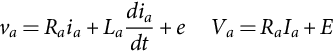
The dynamic and the steady-state responses of the motor and load are given by
DynamicSteady-state
va=Raia+Ladiadt+eVa=RaIa+E
vf=Rfif+LfdifdtVf=RfIf

e=KifωE=KIfω
T=Jdωdt+Dω+TLT=Jω+TL
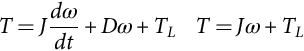
where J,D and TL are the moment of inertia, damping factor, and load torque, respectively, referred to the motor, and the subscripts a and f refer to the armature and field circuits, respectively. R, L, I, and E refer to resistance, inductance, current, and back emf of the motor in associated circuits referred by the subscripts.
Small servo-type dc motors normally have permanent-magnet (PM) excitation for the field, whereas larger size motors tend to have separate field supply, Vf, for excitation. The separately excited dc motors represented in Fig. 30.2A have fixed field excitation, and these motors are very easy to control via the armature current control, which are easily designed using classical linear control theory. Thyristor ac-dc converters with phase-angle control are popular for the larger size motors, whereas the duty-cycle-controlled pulse-width-modulated switching dc-dc converters are popular for servo-motor drives. The series-excited dc motor has its field circuit in series with the armature circuit as shown in Fig. 30.2B. Such a connection gives high torque at a low speed and low torque at a high speed—a pseudo constant-power-like characteristic that may match traction-type loads well.

Torque-speed characteristics of the separately excited and series-excited dc motors are indicated in Fig. 30.3A and B, respectively. The speed of the separately excited dc motor drops with load, the net drop being about 5%–10% of the base speed at full load. The voltage drop across the armature resistance and the armature reaction are responsible for this. Operation of the motor above the base speed at which the armature voltage reaches for the rated field excitation is by means of field weakening, whereby the field current is reduced in order to increase speed beyond the base speed. The armature voltage is now maintained at the rated value actively, by overriding the field control if required. Note that the range of field control is limited because of the magnetic nonlinearity of the field circuit and the problem of good commutation at weak field. Usually, the top speed is limited to about three times the base speed. Note also that field weakening results in reduced torque production per ampere of armature current. Depending on the type of load, the armature current, and speed change as dictated by Eqs. (30.1)–(30.5).

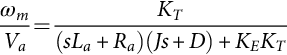
For the separately excited dc motor, assuming that the field excitation is held constant, the transfer characteristic between the shaft speed and the applied voltage to the armature can be expressed as indicated in the block diagram of Fig. 30.4. If we ignore the load torque TL, the transfer characteristic is given by
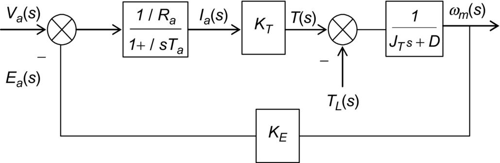
ωmVa=KT(sLa+Ra)(Js+D)+KEKT
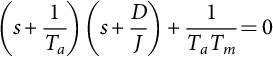
the characteristic roots of which are given by
(s+1Ta)(s+DJ)+1TaTm=0
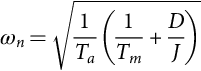
If we compare this with a standard second-order system, the undamped natural frequency and damping factor are given by
ωn=√1Ta(1Tm+DJ)
and
σ=ξωn=12[1Ta+DJ]
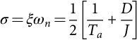
where Tm=mechanical time constant=RaJKEKT![]() in which KE=Kif=KT
in which KE=Kif=KT![]() in SI units and Ta=electric time constant=LaRa
in SI units and Ta=electric time constant=LaRa![]() .
.
The speed response of the motor around an operating speed to the application of load torque on the shaft is given by
ΔωmΔTL=1+sTa(1+sTa)(Js+D)+KEKTRa

30.2.3 Converters for DC Drives
Depending on the application requirements, the power converter for a dc motor may be chosen from a number of topologies. For example, a half-controlled thyristor converter or a single-quadrant pulse-width-modulated (PWM) switching converter may be adequate for a drive that does not require controlled deceleration with regenerative braking. On the other hand, a full four-quadrant thyristor or transistor converter for the armature circuit and a two-quadrant converter for the field circuit may be required for a high-performance drive with a wide speed range.
The frequency at which the power converter is switched, for example, 100 Hz for a single-phase thyristor bridge converter supplied from a 50 Hz ac source (or 300 Hz for a three-phase thyristor bridge converter), 20 kHz for a PWM MOSFET H-bridge converter, and so on, has a profound effect on the dynamics achievable with a motor drive. Low-power switching devices tend to have faster switching capability than high-power devices. This is convenient for low-power motors since these are normally required to be operated with high dynamic response and accuracy.
30.2.3.1 Thyristor Converter Drive
Consider the dc drive of Fig. 30.5 for which the armature supply voltage va to the motor is given by

va=2Vmaxπcosα

where Vmax is the peak value of the line-line ac supply voltage to the converter and α is the firing angle. The dc output voltage va is controllable via the firing angle α, which in turn, is controlled by the control voltage ec as the input to the firing control circuit (FCC). The FCC is synchronized with the mains ac supply and drives individual thyristors in the ac-dc converter according to the desired firing angle. Depending on the load and the speed of operation, the conduction of the current may become discontinuous as indicated in Fig. 30.6A. When this happens, the converter output voltage does not change with the control voltage as proportionately as with the continuous conduction. The motor speed now drops much more with the load as indicated by Fig. 30.6B. The consequent loss of gain of the converter may have to be avoided or compensated if good control over speed is desired.

The output voltage of the simple, two-pulse ac-dc converter of Fig. 30.5 is rich in ripples of frequency nf, where n is an even integer starting with two and f is the frequency of the ac supply. Such low-frequency ripple may derate the motor considerably. Converters with higher pulse number, such as the 6- or 12-pulse converters deliver much smoother output voltage and may be desirable for more demanding applications.
A high-performance dc drive for a rolling mill drive may consist of such converter circuits connected for bidirectional operation of the drive, as indicated in Fig. 30.7. The interfacing of the FCC to other motion-control loops, such as speed and position controllers, for the desired motion is also indicated
Two fully controlled bridge ac-dc converter circuits are used back-to-back from the same ac supply. One is for forward, and the other is for reverse driving of the motor. Since each is a two-quadrant converter, either may be used for regenerative braking of the motor. For this mode of operation, the braking converter, which operates in the inversion mode, sinks the motor current aided by the back emf of the motor. The energy of the overhauling decelerating motor now returns to the ac source.
It may be noted that the braking converter may be used to maintain the braking current at the maximum allowable level right down to zero speed. A complete acceleration-deceleration cycle of such a drive is indicated in Fig. 30.8. During braking, the firing angle is maintained at an appropriate value at all times so that the controlled and predictable deceleration takes place at all times.

The innermost control loop indicated in Fig. 30.7 is for torque, which translates to an armature current loop for a dc drive. Speed- and position-control loops are usually designed as hierarchical control loops. Operation of each loop is sufficiently decoupled from each other so that each stage can be designed in isolation and operated with its special limiting features.
30.2.3.2 PWM Switching Converter Drive
Pulse-width-modulated switching converters have traditionally been referred to as choppers in many traction and forklift-type drives. These are essentially PWM dc-dc converters operating from rectified dc or battery mains. These converters can also operate in one, two, or four quadrants, offering a few choices to meet application requirements. Servo-drive systems normally use the full four-quadrant converter of Fig. 30.9 that allows the bidirectional driving and regenerative braking capabilities.

For forward driving, the transistors T1 and T4 and diode D2 are used as a buck converter that supplies a variable voltage, va, to the armature given by
va=δVDC
where VDC is the dc supply voltage to the converter and δ is the duty cycle of the transistor T1.
The duty cycle δ is defined as the duration of the ON-time of the modulating (switching transistor) as a fraction of the switching period. The switching frequency is normally dictated by the application and the type of switching devices selected for the application.
During regenerative braking in the forward direction, transistors T2 and diode D4 are used as a boost converter that regulates the braking current through the motor by automatically adjusting the duty cycle of T2. The energy of the overhauling motor now returns to the dc supply through the diode D1, aided by the motor back emf and the dc supply. Again, note that the braking converter, comprising T2 and D1, may be used to maintain the regenerative braking current at the maximum allowable level right down to zero speed.
Fig. 30.10 shows a typical acceleration-deceleration cycle of such a drive under the action of the control loops indicated in Fig. 30.9.

Four-quadrant PWM converter drives such as that in Fig. 30.10 are widely used for motion-control equipment in the automation industry. Because of the significant development of power switching devices, switching frequencies of 10–20 kHz are easily attainable. At such frequencies, virtually, no derating of the motor is necessary.
In order to satisfy the requirements of a drive application, simpler versions of the drive circuits indicated in Figs. 30.7 and 30.9 may be used. For instance, for a unidirectional drive, half of the converter circuits indicated earlier may be used. Further simplification of the drive circuit is possible, if regenerative braking is not required.
30.2.4 Drive System Integration
A complete drive system has a torque controller (armature current controller for a dc drive) as its innermost loop, followed by a speed controller as indicated in Fig. 30.11.

The inner current loop is often regulated with a proportional-plus-integral (PI)-type controller of high gain. The rest of the inner loop consists of the converter, the motor armature, which is essentially an R-L circuit with the armature back emf as disturbance and the current sensor. The current sensor is typically an isolated circuit, such as a Hall sensor or a direct-current transformer (DCT). A well-designed torque (armature current) loop behaves essentially as a first-order lag system. Together with the mechanical inertia load, this loop can be indicated as the middle Bode plot of Fig. 30.12, in which 1/T1 represents the current-controlled system bandwidth. (Note that the damping factor D and the load torque TL indicated in Fig. 30.11 have been neglected in this description for simplicity.) The current loop is normally designed by analyzing the block diagram of Fig. 30.11, the converter and the PI controller for the current loop using Bode analysis or other control system design tools.

The next step is usually the design of the speed controller. The 0 db intercept of 1/Js(1+Tis)![]() is normally too low. Again, if a PI controller is selected for the speed loop, its Bode plot is superimposed on the current-controlled system as indicated in Fig. 30.12 to obtain the desired speed-control bandwidth.
is normally too low. Again, if a PI controller is selected for the speed loop, its Bode plot is superimposed on the current-controlled system as indicated in Fig. 30.12 to obtain the desired speed-control bandwidth.
30.2.5 Converter-DC Drive System Considerations
Several operational factors need to be considered in applying a dc drive. Some of the important ones are as follows:
1. The armature current may be rich in harmonics. This is particularly true for thyristor converters. The feedback of these current ripples into the FCC may cause overloading of individual switches and tripping. Adequate filtering is necessary to avoid such problems.
2. Since the converter is switched at regular intervals while the current controller operates continuously, current overshoot may occur because of the delay in the FCC. The current controller gains must be limited to limit this overshoot.
3. The switching frequency of the converter should be selected according to the desired motor-current ripple, supply input current harmonics, and the dynamic performance of the drive.
4. Ripple in the speed-sensor output limits the performance of the speed controller. Analog tachogenerator output is particularly noisy and defines the upper limit of the speed-control bandwidth. Digital speed sensors, such as encoders and resolvers, alleviate this limit significantly.
30.3 Induction Motor Drives
30.3.1 Introduction
The ac induction motor is by far the most widely used motor in the industry. Traditionally, it has been used in constant and variable-speed drive applications that do not cater for fast dynamic processes. Because of the recent development of several new control technologies, such as vector and direct torque controls, this situation is changing rapidly. The underlying reason for this is the fact that the cage induction motor is much cheaper and more rugged than its competitor, the dc motor, in such applications. This section starts with the induction motor drives that are based on the steady-state equivalent circuit of the motor, followed by vector-controlled drives that are based on its dynamic model.
30.3.2 Steady-State Representation
The traditional methods of variable-speed drives are based on the equivalent circuit representation of the motor referred to the stator, as shown in Fig. 30.13.

From this representation, the following power relationships in terms of motor parameters and the rotor slip can be found:
Powerintherotorcircuit,P2=3I′22R′2s=3sR′2E21R′22+(sω1L′2)2
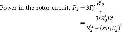
Outputpower,Po=P2−3I′22R′2=(1−s)P2=ω0T=(1−s)ω1pT

where
slip,s=ω1−ωrω1=ω1−pωoω1p=numberofpolepairsωo=2πN60rad/s;Nistherotorspeedinrev/min,ωr=rotorspeedinelectricalrad/s,
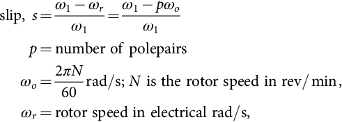
and
ω1=2πf1rad/s(electrical),f1beingthesupplyfrequency.
Thedevelopedtorque,T=P2ω1/pNm

The slip frequency, sf1, is the frequency of the rotor current and the air-gap voltage E1 is given by
E1=ω1LmIm=ω1λm
where λm is the stator flux linkage due to the air-gap flux. If the stator impedance is negligible compared with E1, which is true when f1 is near the rated frequency fo,
V1≈E1=2πf1λm
and
T=3pω1sR′2V21R′22+(sω1L′2)2=3pω1sR′2(2πf1)2λ2mR′22+(sω1L′2)2

30.3.3 Characteristics and Methods of Control
The above analysis suggests several speed-control methods. The following are the widely used methods:
2. Slip power control
3. Variable-voltage, variable-frequency (V-f) control
4. Variable-current, variable-frequency (I-f) control
These methods are sometimes called scalar controls to distinguish them from vector controls, which are described in Section 30.3.4. The torque-speed characteristics of the motor differ significantly under different types of control, as will be evident in the following sections.
30.3.3.1 Stator Voltage Control
In this method of control, back-to-back thyristors are used to supply the motor with variable ac voltage, as indicated in the converter circuit diagram of Fig. 30.14A.
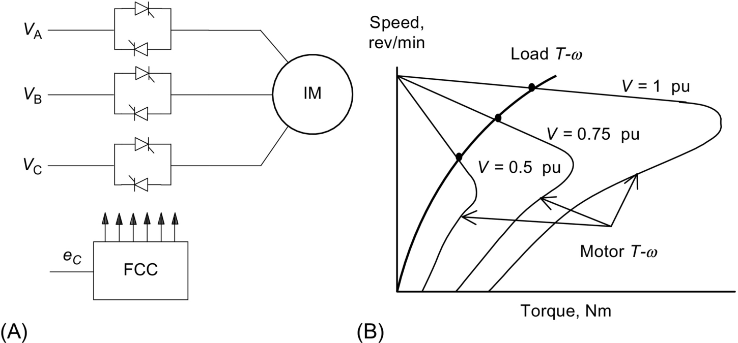
The analysis of Section 30.3.1 implies that the developed torque varies inversely as the square of the input root-mean-square (RMS) voltage to the motor, as indicated in Fig. 30.14B. This makes such a drive suitable for fan- and impeller-type loads for which the torque demand rises faster with speed. For other type of loads, the suitable speed range is very limited. Motors with high rotor resistance may offer an extended speed range. It should be noted that this type of drive with back-to-back thyristors with the firing-angle control suffers from poor power and harmonic distortion factors when operated at a low speed.
If unbalanced operation is acceptable, the thyristors in one or two supply lines to the motor may be bypassed. This offers the possibility of dynamic braking or plugging, desirable in some applications.
30.3.3.2 Slip Power Control
Variable-speed, three-phase, wound-rotor (or slip-ring) induction motor drives with slip power control may take several forms. In a passive scheme, the rotor power is rectified and dissipated in a liquid resistor or in a multitapped resistor that may be adjustable and forced cooled. In a more popular scheme, which is widely used in medium- to large-capacity pumping installations, the rectified rotor power is returned to the ac mains by a thyristor converter operating in a naturally commutated inversion mode. This static Scherbius scheme is indicated in Fig. 30.15. In this scheme, the rotor terminals are connected to a three-phase diode bridge that rectifies the rotor voltage. This rotor output is then inverted into mains frequency ac by a fully controlled thyristor converter operating from the same mains as the motor stator.
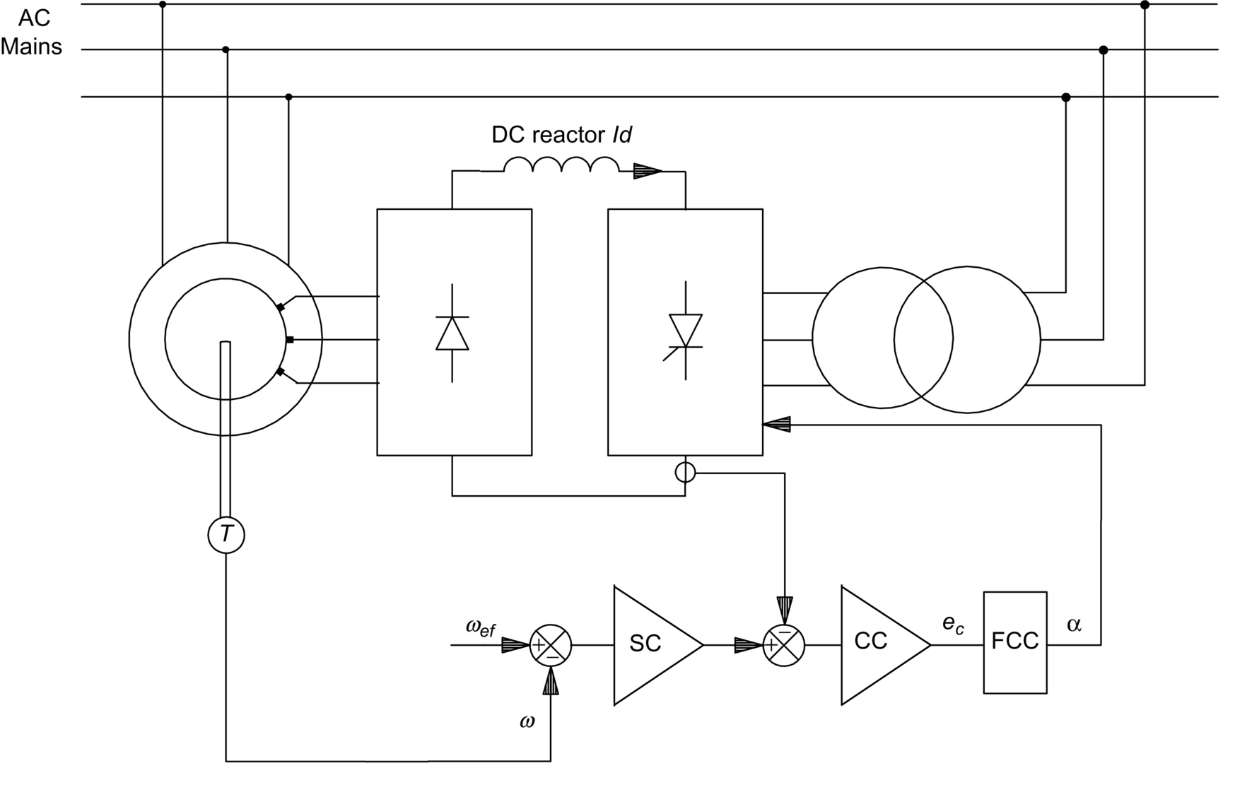
The converter in the rotor circuit handles only the rotor slip power, so that the cost of the power converter circuit can be much less than that of an equivalent inverter drive, albeit at the cost of the more expensive motor. The dc-link current, smoothed by a reactor, may be regulated by controlling the firing angle of the converter in order to maintain the developed torque at the level required by the load. The current controller (CC) and speed controller (SC) are also indicated in Fig. 30.15. The current controller output determines the converter firing angle α from the firing control circuit (FCC).
From the equivalent circuit of Fig. 30.13 and ignoring the stator impedance, the RMS voltage per phase in the rotor circuit is given by
VR=Vsnωrωs=Vsnsωsωs=Vssn

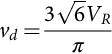
where ωs and ωr are the angular frequencies of the voltages in the stator and rotor circuits, respectively, and n is the ratio of the equivalent stator to rotor turns. The dc-link voltage at the rectifier terminals of the rotor, vd is given by
vd=3√6VRπ
Assuming that the transformer interposed between the inverter output and the ac supply has the same turns ratio n as the effective stator-to-rotor turns of the motor,
vd=−3√6πVsncosα
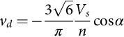
The negative sign arises because the thyristor converter develops negative dc voltage in the inverter mode of operation. The dc-link inductor is mainly to ensure continuous current through the converter so that the expression (30.21) holds for all conditions of operation. Combining the preceding three equations gives
sωs=−ωscosαsothat,s=−ncosα
and the rotor speed
ωo=1p(1−s)ωs=1pωs(1+ncosα)rad/s

Thus, the motor speed can be controlled by adjusting the firing angle α. By varying α between 180° and 90°, the speed of the motor can be varied from zero to full speed, respectively. For a motor with low rotor resistance and with the assumptions taken earlier, it can be shown that the developed torque of the motor is given by
T=3pVsωsid≈3pλmidNm

where id is the dc-link current. Thus, the inner torque-control loop of a variable-speed drive using the Scherbius scheme normally employs a dc-link current loop as the innermost torque loop. Fig. 30.16 shows the transient responses of the dc-link, rotor, and stator currents of such a drive when the motor is accelerated between two speeds.

The drive is normally started with a short-time-rated liquid resistor, and the thyristor speed controller is started when the drive reaches a certain speed.
By replacing the diode rectifier of Fig. 30.16 with another thyristor bridge, power can be made to flow to and from the rotor circuit, allowing the motor to operate at higher than synchronous speed, as is used for grid-connected generator operation in wind power conversion. For very large drives, a cycloconverter may also be used in the rotor circuit with direct conversion of frequency between the ac supply and the rotor and driving the motor above and below synchronous speed.
30.3.3.3 Variable-Voltage, Variable-Frequency (V–f) Control
SPWM inverter drive
When an induction motor is driven from an ideal ac voltage source, its normal operating speed is less than 5% below the synchronous speed, which is determined by the ac source frequency and the number of motor poles. With a sinusoidally modulated (SPWM) inverter, indicated in Fig. 30.17, the supply frequency to the motor can be easily adjusted for variable speed. Eq. (30.18) implies that, if rated air-gap flux is to be maintained at its rated value at all speeds, the supply voltage V1 to the motor should be varied in proportion to the frequency f1, when the voltage drop across the stator resistance can considered to be negligible. The block diagram of Fig. 30.18A shows how the frequency f1 and the output voltage V1 of the SPWM inverter are proportionately adjusted with the speed reference. The speed reference signal is normally passed through a filter that only allows a gradual change in the frequency f1. This type of control is widely referred to as the V-f inverter drive. Control of the stator input voltage V1 as a function of the frequency f1 is readily arranged within the inverter by modulating the switches T1−T6![]() . At a low speed, however, where the input voltage V1 is low, most of the input voltage may drop across the stator impedance, leading to a reduction in air-gap flux and loss of torque.
. At a low speed, however, where the input voltage V1 is low, most of the input voltage may drop across the stator impedance, leading to a reduction in air-gap flux and loss of torque.


Compensation for the stator resistance drop, as indicated in Fig. 30.18B, is often employed. However, if the motor becomes lightly loaded at a low speed, the air-gap flux may exceed the rated value, causing the motor to overheat.
From the equivalent circuit of Fig. 30.13 and neglecting the rotor leakage inductance, the developed torque T and the rotor current I′2 are given by
I2=E1sω1R′2ω1=λmR′2sω1A

and
T=3pR′2ωrI′22Nm

where s ω1 is the slip frequency, which is also the frequency of the voltages and currents in the rotor. Eq. (30.24) implies that by limiting the slip s, the rotor current can be limited, which in turn limits the developed torque Eq. (30.25). Consequently, a slip-limited drive is also a torque-limited drive. Note that this is true only in the steady state. A speed-control system with such a slip limiter is shown in Fig. 30.19. In this scheme, the motor speed is sensed and added to a limited speed error (or limited slip speed) to obtain the frequency (or speed reference for the V-f drive).

Many applications of the V-f controller, however, are open-loop schemes, in which any demanded variation in V1 is passed through a ramp limiter (or filter) so that sudden changes in the slip speed ωr are precluded, thereby allowing the motor to follow the change in the supply frequency without exceeding the rotor current and torque limits.
From the foregoing analyses, it is obvious that the V-f inverter drive essentially operates in all four quadrants, with rotor speed dropping slightly with the load and developing full torque at the same slip speed at all speeds. This assumes that the stator input voltage is properly compensated, so that the motor is operated with constant (or rated) air-gap flux at all speed. The motor can be operated above the base speed by keeping the input voltage V1 constant, while increasing the stator frequency above base frequency in order to run the motor at speeds higher than the base speed. The air-gap flux and hence the maximum developed torque now fall with speed, leading to constant-power-type characteristic. Fig. 30.20 depicts the T−ω![]() characteristics of such a voltage- and frequency-controlled drive for various operating frequencies. In this figure, the T−ω
characteristics of such a voltage- and frequency-controlled drive for various operating frequencies. In this figure, the T−ω![]() characteristic for base speed has been drawn in full, indicating the maximum developed torque Tmax and the rated torque. Below base speed, the V1−f1
characteristic for base speed has been drawn in full, indicating the maximum developed torque Tmax and the rated torque. Below base speed, the V1−f1![]() ratio is maintained to keep the air-gap flux constant. Above base speed, V1 is kept constant, while f1 increases with speed, thus weakening the air-gap flux. Forward driving in quadrant 1 takes place with the inverter output voltage sequence of a−b−c
ratio is maintained to keep the air-gap flux constant. Above base speed, V1 is kept constant, while f1 increases with speed, thus weakening the air-gap flux. Forward driving in quadrant 1 takes place with the inverter output voltage sequence of a−b−c![]() , whereas reverse driving in quadrant 3 takes place with the sequence a−b−c
, whereas reverse driving in quadrant 3 takes place with the sequence a−b−c![]() . Regenerative braking while forward driving takes place by adjusting the input frequency f1 in such a way that the motor operates in quadrant 2 (quadrant 4 for reverse braking) with the desired braking characteristic.
. Regenerative braking while forward driving takes place by adjusting the input frequency f1 in such a way that the motor operates in quadrant 2 (quadrant 4 for reverse braking) with the desired braking characteristic.

 characteristics of V-f drive with the input frequency f1 and voltage V1 below and above base speed.
Note that the characteristics in Fig. 30.20 are based on the steady-state equivalent circuit model of the motor. Such a drive suffers from the poor torque response during transient operation because of time-dependent interactions between the stator and rotor fluxes. Fig. 30.21 indicates the machine air-gap flux during acceleration with V-f control obtained from a dynamic model. Clearly, the air-gap flux does not remain constant during the dynamic operation.

Cycloconverter drive
For large-capacity induction motor drives, the variable-frequency supply at variable voltage is effectively obtained from a cycloconverter in which a back-to-back thyristor converter pairs are used, one for each phase of the motor, as indicated in Fig. 30.22. Each thyristor block in this figure represents a fully controlled thyristor ac-dc converter. The maximum output frequency of such a converter can be as high as about 40% of the supply frequency. In view of the large number of thyristor switches required, cycloconverter drives are suitable for large-capacity but low-speed applications.

30.3.3.4 Variable Current–Variable Frequency (I–f) Control
In this scheme, medium- to large-capacity induction motors are driven from a variable but stiff current supply that may be obtained from a thyristor converter and a dc-link inductor as indicated in Fig. 30.23. The frequency of the current supply to the motor is adjusted by a thyristor converter with auxiliary diodes and capacitors. The diodes in each inverter leg and the capacitors across them are needed for turning off the thyristors when current is to be commutated from one to the next in sequence. The motor-current waveforms are normally six-step, or quasi-square, as indicated in Fig. 30.24. The switching states of the inverter thyristors are also indicated in this figure. The motor voltage waveforms are determined by the load. These waveforms are more nearly sinusoidal than the current waveforms.
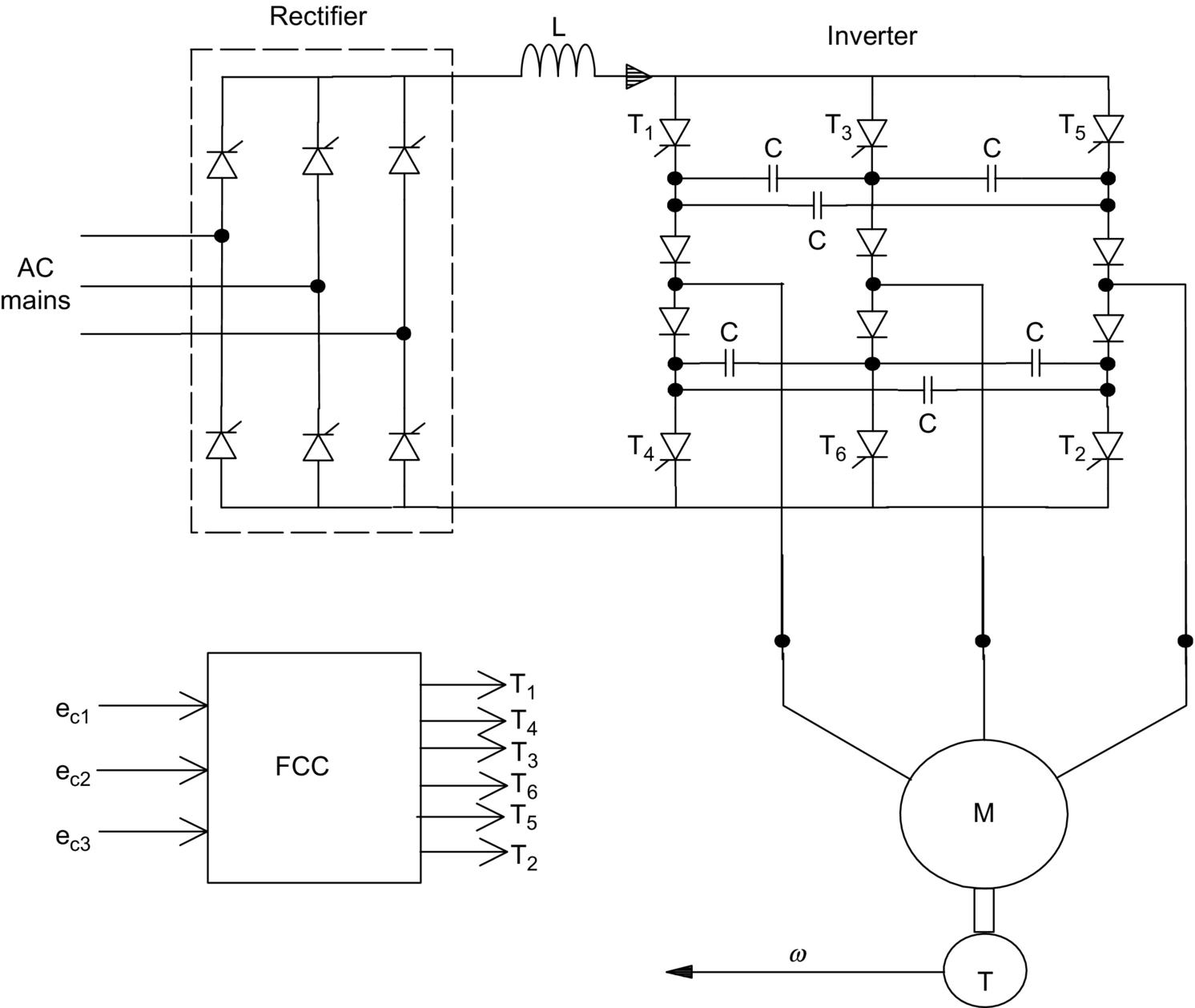

The thyristor converter supplying the quasi-square current waveforms to the motor has firing-angle control, in order to regulate the dc-link current to the inverter. The dynamics of the dc-link current control is such that this current may be considered to be constant during the time the inverter switches commutate the dc-link current from one switch to the next. Such a current-source drive offers four-quadrant operation, with independent control of the dc-link current and output frequency. One drawback is that the motor voltage waveforms have voltage spikes due to commutation.
From the analysis of Section 30.3.2, if the higher order harmonics of the current waveforms in Fig. 30.24 are neglected and it is assumed that the motor voltage and current waveforms are sinusoidal, the magnetizing current Im in Fig. 30.13 can be kept constant (for constant air-gap flux operation) if the RMS value of the stator supply current I1 is defined according to Eq. (30.26). This relationship is also shown in graphic form in Fig. 30.25.

Im=I1[R′22+(2πf1sL′2)2R′22+2πf1(L′2+Lm)2]1/2=constant

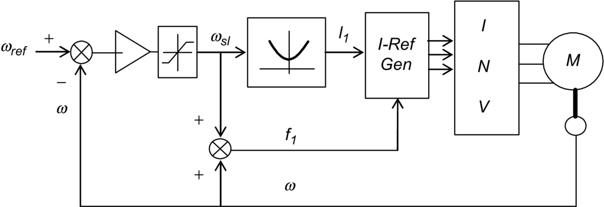
The control scheme for variable-speed operation with a current-source drive is indicated in the block diagram of Fig. 30.26. The speed reference defines the stator current reference according to Eq. (30.26), and the frequency reference is obtained by adding the rotor frequency to the actual speed of the motor. The inverter drive may consist of the thyristor current source and the inverter of Fig. 30.23 or a diode rectifier supplied SPWM transistor inverter of Fig. 30.17 with independent current regulators, one for each phase.
The dynamic performance of such current-controlled induction motor drives is not very satisfactory, just as for the voltage-source inverters. Furthermore, the current-source inverter drive cannot normally be operated open loop, like the V-f inverter drive. For high dynamic performance, vector-controlled drives are becoming popular.
30.3.4 Vector Controls
The foregoing scalar control methods are only suitable for adjustable-speed applications in which the load speed or position is not controlled like in a servo system. Instantaneous frequency control with a view to control motor speed or position cannot be defined, and therefore, instantaneous torque control cannot be addressed by scalar control methods. Vector control technique allows a squirrel-cage induction motor to be driven with high dynamic performance, comparable with that of a dc motor. In vector control, machine dynamic model rather than steady-state model (on which scalar controllers are based on) is used to design the controller. For this, the controller needs to know the rotor speed (in the indirect method) or the air-gap flux vector (in the direct method) accurately, using sensors. The latter method is not practical because of the requirement of attaching air-gap flux sensors. The indirect method, which is being widely accepted in recent years, requires the controller to be matched with the motor being driven. This is because the controller also needs to know some rotor parameter(s), which may vary according to the conditions of operation, continuously.
30.3.4.1 Basic Principles
The methods of vector control are based on the dynamic equivalent circuit of the induction motor. There are at least three fluxes (rotor, air gap, and stator) and three currents or mmfs (stator, rotor, and magnetizing) in an induction motor. For high dynamic response, interactions among current, fluxes, and speed, must be taken into account in determining appropriate control strategies. These interactions are understood only via the dynamic model of the motor.
All fluxes rotate at synchronous speed. The three-phase currents create mmfs (stator and rotor) that also rotate at synchronous speed. Vector control aligns axes of an mmf and a flux orthogonally at all times. It is easier to align the stator current mmf orthogonally to the rotor flux.
Any three-phase sinusoidal set of quantities in the stator can be transformed to an orthogonal reference frame by
[fαsfβsfo]=23[cosθcos(θ−2π3)cos(θ−4π3)sinθsin(θ−2π3)sin(θ−4π3)121212][fasfbsfcs]

where θ is the angle of the orthogonal set α−β−0![]() with respect to any arbitrary reference. If the α−β−0
with respect to any arbitrary reference. If the α−β−0![]() axes are stationary and the α-axis is aligned with the stator α-axis, then θ=0
axes are stationary and the α-axis is aligned with the stator α-axis, then θ=0![]() at all times. Thus,
at all times. Thus,
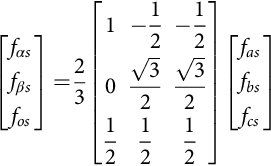
[fαsfβsfos]=23[1−12−120√32√32121212][fasfbsfcs]
If the orthogonal set of reference rotates at the synchronous speed ω1, its angular position at any instant is given by
θ=∫t0ω1t+θo

The orthogonal set is then referred to as d−q−0![]() axes. The three-phase rotor variables, transformed to the synchronously rotating frame, are
axes. The three-phase rotor variables, transformed to the synchronously rotating frame, are
[fdrfqrfo]=23[cos(ωe−ωr)tcos((ωe−ωr)t−2π3)cos((ωe−ωr)t−4π3)sin(ωe−ωr)tsin((ωe−ωr)t−2π3)sin((ωe−ωr)t−4π3)121212]×[farfbrfcr]
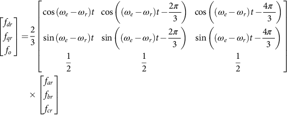
It should be noted that the difference ωe−ωr![]() is the relative speed between the synchronously rotating reference frame and the frame attached to the rotor. This difference is also the slip frequency, ωsl, which is the frequency of the rotor variables. By applying these transformations, voltage equations of the motor in the synchronously rotating frame reduce to
is the relative speed between the synchronously rotating reference frame and the frame attached to the rotor. This difference is also the slip frequency, ωsl, which is the frequency of the rotor variables. By applying these transformations, voltage equations of the motor in the synchronously rotating frame reduce to
[vqsvdsvqrvdr]=[Rs+pLsωeLspLmωeLm−ωeLsRs+pLs−ωeLmpLmpLm(ωe−ωr)LmRr+pLr(ωe−ωr)Lr−(ωe−ωr)pLm−(ωe−ωr)LrRr+pLr]×[iqsidsiqridr]

where the speed of the reference frame, ωe, is equal to ω1 and Ls=Lls+Lm,Lr=Llr+Lm.![]()
Subscripts l and m stand for leakage and magnetizing, respectively, and p represents the differential operator d/dt, not the number of pole pairs. The equivalent circuits of the motor in this reference frame are indicated in Fig. 30.27A and B.

The stator flux linkage equations are
λqs=Llsiqs+Lm(iqs+iqr)=Lsiqs+Lmiqr
λds=Llsids+Lm(ids+idr)=Lsids+Lmidr
ˆλs=√(λ2qs+λ2ds)

The rotor flux linkages are given by
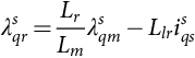
λqr=Llriqr+Lm(iqs+iqr)=Lriqr+Lmiqs
λdr=Llridr+Lm(ids+idr)=Lridr+Lmids
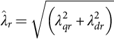
ˆλr=√(λ2qr+λ2dr)
The air-gap flux linkages are given by
λmq=Lm(iqs+iqr)
λmd=Lm(ids+idr)
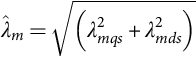
ˆλm=√(λ2mqs+λ2mds)
The torque developed by the motor is given by
T=3p2[λdsiqs−λqsids]
where p is the number of pole pairs.
From Eq. (30.31), the rotor voltage equations are
vqr=0=Lmdiqsdt+(ωe−ωr)Lmids+(Rrir+Lrdiqrdt)+(ωe−ωr)Lridr

vdr=0=Lmdidsdt+(ωe−ωr)Lmiqs+(Rrir+Lrdidrdt)+(ωe−ωr)Lriqr

Using Eqs. (30.35) and (30.36),
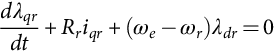
dλqrdt+Rriqr+(ωe−ωr)λdr=0
anddλdrdt+Rridr+(ωe−ωr)λqr=0

Also from Eqs. (30.35) and (30.36),
iqr=1Lrλqr−LmLriqs

idr=1Lrλdr−LmLrids

The rotor currents iqr and idr can be eliminated from Eqs. (30.44) and (30.45) by using Eqs. (30.46) and (30.47). Thus,
dλqrdt+LrRrλqr−LmLrRriqs+(ωe−ωr)λdr=0

dλdrdt+RrLrλdr−LmLrRrids+(ωe−ωr)λqr=0

The elimination of transients in rotor flux and the coupling between the two axes occurs when
λqr=0andˆλr=λdr
The rotor flux should also remain constant so that
dλdrdt=0=dλqrdt

From Eq. (30.48) to Eq. (30.51),
ωe−ωr=ωsl=LmˆλrRrLriqs

andLrRrdˆλrdt+ˆλr=Lmids

Substituting the expressions for iqr and idr into Eqs. (30.35) and (30.36),
λqs=(Ls−L2mLr)iqs+LmLrλqr

λds=(Ls−L2mLr)ids+LmLrλdr

Substituting λqs and λds from Eqs. (30.54) and (30.55) into the torque equation of Eq. (30.41),
T=3P2LmLr(λdriqs−λqrids)=3P2LmLrˆλriqs

It is clear from Eq. (30.53) that the rotor flux ˆλdr![]() is determined by ids, subject to a time delay Tr, which is the rotor time constant (Lr/Rr). The current iqs, according to Eq. (30.56), controls the developed torque T without delay. Currents ids and iqs are orthogonal to each other and are called the flux- and torque-producing currents, respectively. This correspondence between the flux- and torque-producing currents is subject to maintaining the conditions in Eqs. (30.50) and (30.51). Normally, ids would remain fixed for operation up to the base speed. Thereafter, it is reduced in order to weaken the rotor flux so that the motor may be driven with a constant-power-like characteristic.
is determined by ids, subject to a time delay Tr, which is the rotor time constant (Lr/Rr). The current iqs, according to Eq. (30.56), controls the developed torque T without delay. Currents ids and iqs are orthogonal to each other and are called the flux- and torque-producing currents, respectively. This correspondence between the flux- and torque-producing currents is subject to maintaining the conditions in Eqs. (30.50) and (30.51). Normally, ids would remain fixed for operation up to the base speed. Thereafter, it is reduced in order to weaken the rotor flux so that the motor may be driven with a constant-power-like characteristic.
Based on how the rotor flux is detected and regulated, two methods of control are available. One is the more popular indirect rotor-flux-oriented control (IFOC) method, and the other is the direct vector control method; both are described hereafter.
30.3.4.2 Indirect Rotor Flux Oriented (IFOC) Vector Control
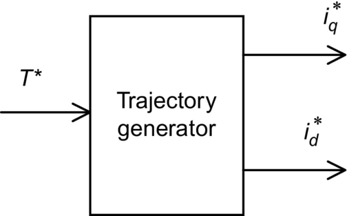
In the indirect scheme, the relationship between the slip frequency and current iqs given by Eq. (30.52) is used to relate the compensated speed error ω1−ωr![]() to iqs. The iqs, in turn, is used to develop to the demanded torque T⁎ according to the Eq. (30.56). The rotor flux is maintained at the base value for operation below speed, and it may be reduced to a lower value for field weakening above base speed. The orthogonal relationship between the torque-producing stator current iqs and the flux-producing stator current ids is maintained at all times by generating the stator current references in the synchronously rotating dq reference frame, using sine and cosine functions of angle θ1. This angle is obtained as indicated in Fig. 30.28.
to iqs. The iqs, in turn, is used to develop to the demanded torque T⁎ according to the Eq. (30.56). The rotor flux is maintained at the base value for operation below speed, and it may be reduced to a lower value for field weakening above base speed. The orthogonal relationship between the torque-producing stator current iqs and the flux-producing stator current ids is maintained at all times by generating the stator current references in the synchronously rotating dq reference frame, using sine and cosine functions of angle θ1. This angle is obtained as indicated in Fig. 30.28.
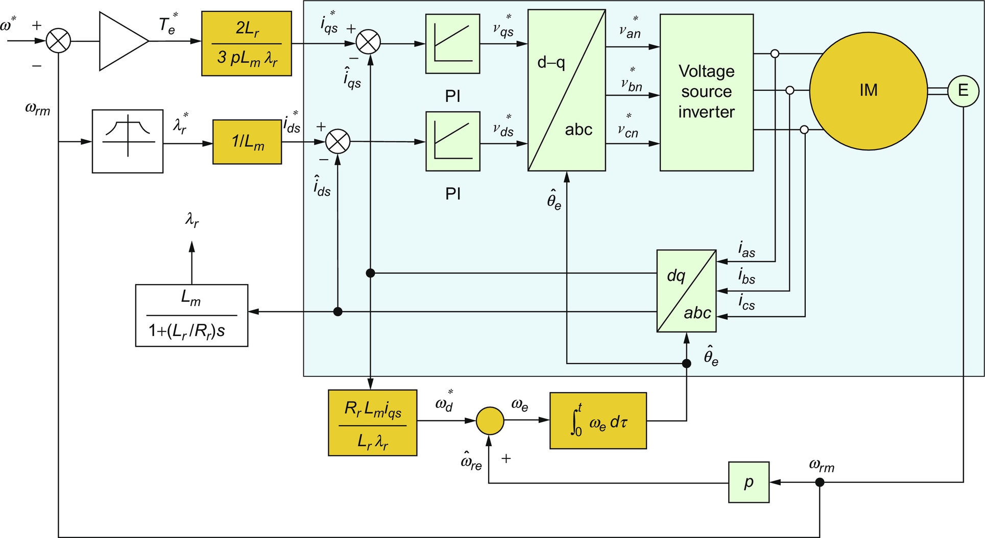
The compensated speed error produces the current reference i∗qs![]() according to Eq. (30.56). The current reference i∗qs
according to Eq. (30.56). The current reference i∗qs![]() also gives the slip speed ωsl, according to Eq. (30.53). The slip speed ωsl is added to the rotor speed ω, to obtain the stator frequency ω1. This frequency is integrated with respect to time to produce the required angle θ1 of the stator mmf relative to the rotor flux vector. This angle is used to transform the stator currents to the dq reference frame. Two independent current controllers are used to regulate the iq and id currents to their reference values. The compensated iq and id errors are then inverse transformed into the stator a−b−c
also gives the slip speed ωsl, according to Eq. (30.53). The slip speed ωsl is added to the rotor speed ω, to obtain the stator frequency ω1. This frequency is integrated with respect to time to produce the required angle θ1 of the stator mmf relative to the rotor flux vector. This angle is used to transform the stator currents to the dq reference frame. Two independent current controllers are used to regulate the iq and id currents to their reference values. The compensated iq and id errors are then inverse transformed into the stator a−b−c![]() reference frame for obtaining switching signals for the inverter via PWM or hysteresis comparators.
reference frame for obtaining switching signals for the inverter via PWM or hysteresis comparators.
It is clear that this scheme uses a feedforward scheme, or a machine model, in which the current reference for iqs is also determined by the rotor time constant Tr. This is also indicated in Fig. 30.28. The rotor time constant Tr cannot be expected to remain constant for all conditions of operation. Its considerable variation with operating conditions means that the slip speed ωsl, which directly affects the developed torque and the rotor flux vector position, may vary widely. Many rotor time-constant identification schemes have been developed in recent years to overcome the problem.
The mandatory requirement for a rotor-speed sensor is also a significant drawback, because its presence reduces the reliability of the IFOC drive. Consequently, sensorless schemes of identifying the rotor flux position have also drawn considerable interest in recent years.
Fig. 30.29 shows the transient response of an induction motor under the IFOC drive scheme of Fig. 30.28. In this case, the drive accelerates a large inertia load from standstill to the base speed of 1500 rev/min. It is clear that the overcurrent transients of Fig. 30.21 are eliminated, while the motor accelerates under a constant torque (implied by the constant rate at which the speed increases) and settles at the final speed with little over- or undershoot in speed. Clearly, rotor and air-gap fluxes remain constant at all times.

30.3.4.3 Direct Vector Control with Airgap Flux Sensing
In the direct scheme, use is made of the air-gap flux linkages in the stator d- and q-axes, which are then compensated for the respective leakage fluxes in order to determine the rotor flux linkages in the stator reference frame. The air-gap flux linkages are measured by installing quadrature flux sensors in the air gap, as indicated in Fig. 30.30.

By returning to Eqs. (30.32)–(30.40) in the stator reference frame and using some simplifications, it can be shown that
λsqr=LrLmλsqm−Llrisqs
λsdr=LrLmλsdm−Llrisds

where the superscript s stands for the stator reference frame. Since the rotor flux rotates at a synchronous speed with respect to the stator reference frame, the angle θ1 used for the coordinate transformations in Fig. 30.27 can be obtained from
cosθ1=λsdrˆλr

andsinθ1=λsqrˆλr
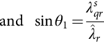
where |ˆλr|=√(λ2dr)2+(λsqr)2![]() .
.
The control of torque via iqs and the rotor flux via ids, subject to satisfying conditions (30.50) and (30.51), remain as indicated in Fig. 30.28, according to the basic principle of vector control.
The requirement of air-gap flux sensors is rather restrictive. Such fittings also reduce reliability. Even though this method of control offers better low-speed performance than the IFOC, this restriction has practically precluded the adoption of this scheme. In an alternative method, the d- and q-axes stator flux linkages of the motor may be computed from integrating the stator input voltages.
30.4 Synchronous Motor Drives
30.4.1 Introduction
Variable-speed synchronous motors have been widely used in very large-capacity (>MW![]() ) pumping and centrifuge-type applications using naturally commutated current-source thyristor converters. At the low-power end, the current-source SPWM inverter-driven synchronous motors have become very popular in recent years in the form of permanent-magnet brushless dc and ac synchronous motor drives in servo-type applications. There are certain features of three-phase synchronous motors that have allowed them, especially the lower capacity motors, to be controlled with high dynamic performance using cheaper control hardware than is required for the induction motor of similar capacity. Since the average speed of the synchronous motor is precisely related to the supply frequency, which can be precisely controlled, multimotor drives with a fixed speed ratio among them are also good candidates for synchronous motor drives. This section begins with the performance of the variable-speed nonsalient-pole and salient-pole synchronous motor drive using the steady-state equivalent circuit followed by the dynamics of the vector-controlled synchronous motor drive.
) pumping and centrifuge-type applications using naturally commutated current-source thyristor converters. At the low-power end, the current-source SPWM inverter-driven synchronous motors have become very popular in recent years in the form of permanent-magnet brushless dc and ac synchronous motor drives in servo-type applications. There are certain features of three-phase synchronous motors that have allowed them, especially the lower capacity motors, to be controlled with high dynamic performance using cheaper control hardware than is required for the induction motor of similar capacity. Since the average speed of the synchronous motor is precisely related to the supply frequency, which can be precisely controlled, multimotor drives with a fixed speed ratio among them are also good candidates for synchronous motor drives. This section begins with the performance of the variable-speed nonsalient-pole and salient-pole synchronous motor drive using the steady-state equivalent circuit followed by the dynamics of the vector-controlled synchronous motor drive.
30.4.2 Steady-State Equivalent-Circuit Representation of the Motor
Some of the operating characteristics of variable-frequency voltage- and current-source-driven synchronous motors can be readily obtained from their steady-state equivalent representation, as was the case with the scalar controls of induction motor drives. Assuming balanced, sinusoidal distribution of stator and rotor mmfs and a uniform air-gap (nonsalient-pole motor), the per-phase equivalent circuit of Fig. 30.31 represents the motor at a constant speed.

The representation in Fig. 30.31 is in terms of the RMS voltage V applied to the motor phase winding that consists of the phase resistance R, the synchronous reactance Xs (in Ω/phase), and the per-phase induced voltage Ef. The back emf Ef develops in the stator phase winding as a result of rotor excitation supplied from an external dc source via slip rings or by permanent magnets in the rotor. The phasor Ef has an arbitrary phase angle δ with respect to the input voltage V. This is the load angle of the motor.
Unlike the induction motor, a synchronous motor may derive part or all of its excitation from the rotor via rotor excitation. For small synchronous motors that are used in the brushless dc and ac servo applications, this excitation is derived from permanent magnets in the rotor. This is readily and economically obtained with the modern permanent magnets, thus dispensing with the slip-ring-brush assembly. The i2R losses in the rotor windings with the external excitation are also eliminated. These magnets also allow considerable reduction in space requirement for the rotor excitation. For large synchronous motors, this excitation is supplied more economically from an external dc source via slip rings or via an exciter.
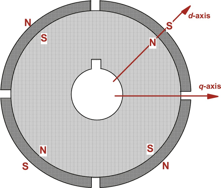
The phasor diagrams of Fig. 30.32 may be used to analyze characteristics of the nonsalient-pole synchronous motor drive. Since the rotor magnetic field may be such that the motor may develop a back emf that is smaller or larger than the ac supply voltage to the stator windings, the motor may accordingly be underexcited or overexcited, respectively. The overexcited motor will normally operate at a leading power factor, as is the case in Fig. 30.32B. This is desirable in high-power applications.

In the phasor diagrams of Fig. 30.32C, the stator current I has been resolved into two components Id and Iq, which are current phasors responsible for developing mmfs in the rotor d- and q-axes. These representations are in the stator reference frame, and hence are sinusoidal quantities at the frequency of the stator supply.
If the voltage drop across the stator resistance is neglected, which may be acceptable when the stator frequency is near the base frequency or higher, the developed torque T of the motor can be found from the phasor relationships of Fig. 30.32. Thus
T=3ωrEVXssinδ=3PωEVωLssinδ=3PKϕLsVωsinδNm
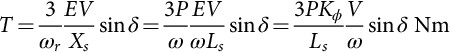
for the nonsalient-pole motor (also for the sine wave PM ac motor with rotor magnets at the surface of the rotor) and
T=3Pωr[EVωLdsinδ+V22(Ld−LqωLdLq)sin2δ]=3P[KϕLdVωsinδ+V22ω2(Ld−LqLdLq)sin2δ]Nm
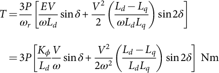
for the salient-pole motor (also for the interior-magnet motor in which the rotor magnets are buried inside the rotor). Here, the flux constant of the motor, Kϕ, is the ratio of the RMS value of the phase voltage Ef induced in the stator only due to the rotor excitation and speed. Note that for a given rotor excitation, the ratio Kϕ=Ef/ω![]() remains constant at all speed.
remains constant at all speed.
30.4.3 Performance with Voltage-Source Inverter Drive
Eqs. (30.61) and (30.62) imply that if the motor is driven from a voltage-source supply and if the input voltage to frequency ratio, V-f, is kept constant, the motor will develop the same maximum torque at all speeds. For the nonsalient-pole motor, this maximum torque will occur for a load angle δ=90°![]() . For the salient-pole motor, this will occur for a load angle, which is also influenced by the relative values of Ld and Lq.
. For the salient-pole motor, this will occur for a load angle, which is also influenced by the relative values of Ld and Lq.
At a low speed, where the supply voltage V is small, the voltage drop in the stator resistance may become significant compared with Ef. This may lead to a significant drop in the maximum available torque, as given by the torque Eqs. (30.63) and (30.64), which are derived from the phasor diagrams of Fig. 30.32. The stator per-phase resistance R is now included in the analysis. The developed torque is then given by
T=3PEfoV1ωoλXsosinδ+R(cosδ−λEfoV1)R2+(λXso)2Nm

for the nonsalient-pole motor and
T=3Pωo[V21λR+VEfoλXqosinδ+V22(Xdo−Xqo)sin2δ−VREfocosδR2+λ2XdXq]Nm
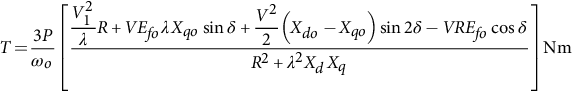
for the salient-pole motor where the subscript o refers to the base quantities and λ refers to the per unit input frequency f1/f0.
Eqs. (30.63) and (30.64) indicate that the maximum torque that the motor can develop diminishes at a low speed because of the voltage drop across the stator resistance R. This drop in maximum available torque at a low speed can be avoided by boosting the input voltage at a low speed, as indicated in Fig. 30.33A. This voltage boosting is similar to the IR compensation applied to a variable-frequency induction motor drive.
 characteristics with a limited maximum δ for constant-power operation.
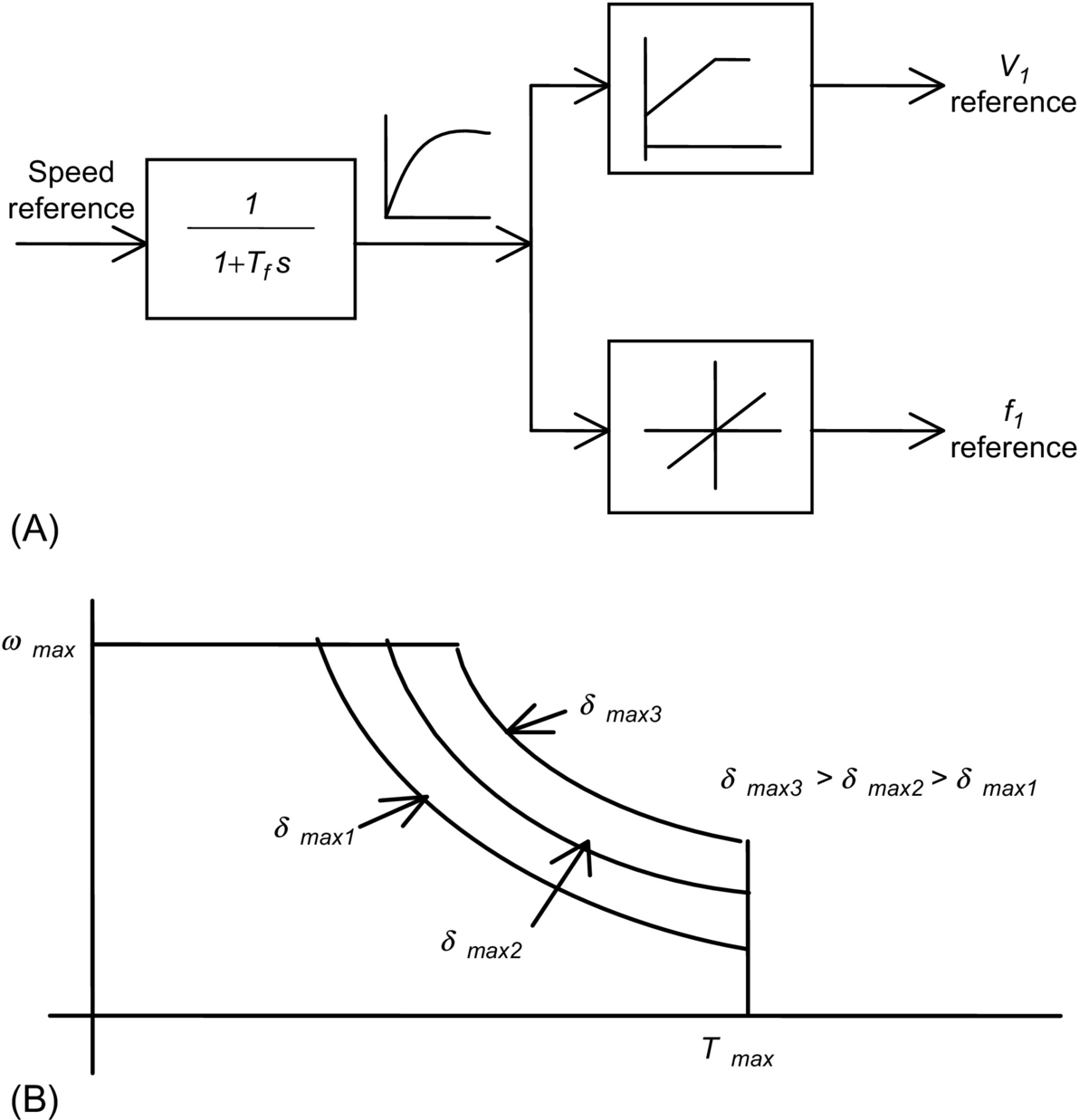
Fig. 30.33 indicates an open-loop V-f inverter drive scheme, similar to the scheme for an induction motor drive in which the RMS stator input voltage is made proportional to frequency. The speed reference is passed through a first-order filter, as shown in Fig. 30.33A, so that a large and abrupt change in the input frequency command to the inverter is avoided. The filtered speed reference is translated into a proportional frequency reference f1. The voltage reference V1 is also proportional to frequency reference but with a zero frequency bias. The variable RMS input voltage V1 to the motor may be obtained from an inverter by SPWM methods or from a cycloconverter with phase-angle control.
The available input voltage V1 is normally limited by the available dc-link voltage to the inverter or the ac supply voltage to a cycloconverter. This limit is normally arranged to occur at base speed. Above this speed, the stator flux drops leading to field weakening and constant-power-like operation, as indicated in Fig. 30.33B. In some control scheme, the maximum load angle δ is not allowed to exceed a certain limiting value δmax. By selecting δmax, constant-power operation at various power levels is possible.
30.4.4 Characteristics Under Current-Source Inverter (CSI) Drive
A CSI-driven synchronous motor drive generally gives higher dynamic response. It also gives better reliability because of the automatic current-limiting feature. In a variable-speed application, the synchronous motor is normally driven from a stiff current source. A rotor-position sensor is used to place the phase current phasor I of each phase at a suitable angle with respect to the back-emf phasor (Ef) of the same phase. The rotor-position sensor is thus mandatory.
Two converter schemes have generally been used. In one scheme, as indicated in Fig. 30.34, a large dc-link reactor (inductor) makes the current source to the inverter stiff. The scheme is suitable for large synchronous motors for which thyristor switches are used in the inverter. A current loop may also be established by sensing the dc-link current and by using a closed-loop current controller that continuously regulates the firing angle of the controllable rectifier in order to supply the inverter with the desired dc-link current. It can be shown that the motor-developed torque is proportional to the level of the dc-link current.

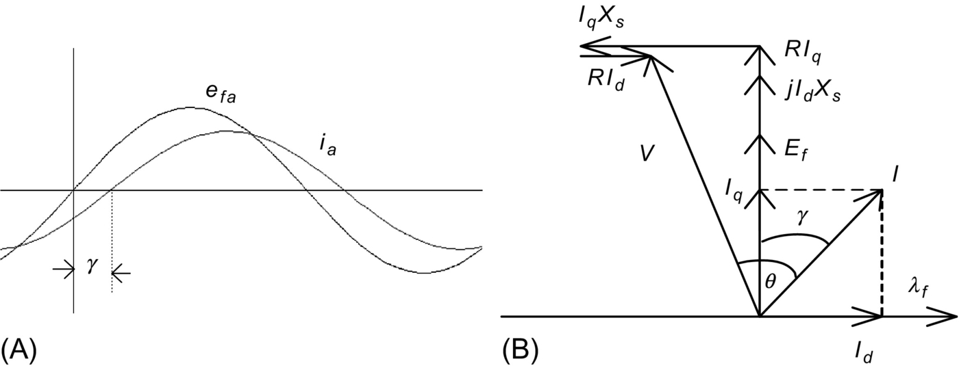
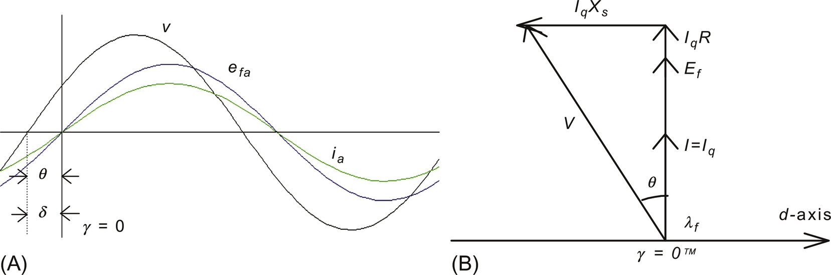
The inverter drives the motor with quasi-square-wave current waveforms as indicated in Fig. 30.35. The current waveforms are switched according to the measured rotor-position information, such that the current waveform in each phase has a fixed angular displacement, γ, with respect to the induced emf of the corresponding phase. Because of this, the drive is sometimes referred to as self-controlled. The angular displacement of these current waveforms (or their fundamental components) with the respective back-emf waveforms is indicated in Fig. 30.35. Because of the large dc-link inductor, the phase currents may be considered to remain essentially constant between the switching intervals. The quasi-square current waveforms contain many harmonics, and are responsible for large torque pulsations that may become troublesome at a low speed.


In the foregoing scheme, the motor can be reversed easily by reversing the sequence of switching of the inverter. It can also be braked regeneratively by increasing the firing angle of the input rectifier beyond 90° while maintaining the dc-link current at the desired braking level until braking is no longer required. The rectifier now returns the energy of the overhauling load to the ac mains regeneratively.
In another scheme, which is preferred for lower capacity drives for which higher dynamic response is frequently sought, phase currents are regulated within the inverter. The inverter typically employs gate turnoff switches, such as the IGBT, and pulse-width modulation techniques, as indicated in Fig. 30.36. Motor currents are sensed and used to close independent current controllers for each phase. Normally, two current controllers suffice for a balanced star-connected motor. Three-phase sinusoidal ac currents are supplied to the motor, the amplitude and phase angle of which can be independently controlled as required. The references for the current controllers are obtained from a three-phase current reference generator that is addressed by the feedback of the rotor position. The rotor position is continuously measured by a high-resolution encoder. In this way, the current references and hence the actual stator currents are synchronized to the rotor.

30.4.5 Brushless DC Operation of the CSI-Driven Motor
The torque characteristic of the CSI drive scheme of the foregoing section can be easily analyzed using the phasor diagrams shown earlier, if the harmonics in the motor-current waveform are neglected or if the motor-current waveforms are indeed sinusoidal as in the second scheme described earlier. In the following analysis, it is assumed that the supply current waveforms are sinusoidal. It is also assumed that the phase angle of these current sources with respect to the induced voltage in each phase can be arbitrarily chosen.
The phase back-emf and the current waveforms and the phasor diagram of the nonsalient-pole motor are shown in Fig. 30.37. The phase angle γ between the Ef and I phasors and the RMS value (or amplitude) of I are determined according to the desired torque and power factor considerations. The developed torque is found from the phasor diagram to be

T=3EfIcosγωr=KϕIcosγNm

If the angle γ=0°![]() is chosen, the familiar dc-motor-like torque characteristic is obtained. It should be noted from the foregoing that the developed torque at any speed is independent of R since a high-gain (stiff) current-source drive is used. Note also that the ratio Ef/ω at any operating speed is proportional to the amplitude of the stator flux linkage, λf, due to rotor excitation. For fixed rotor excitation, this ratio is a constant.
is chosen, the familiar dc-motor-like torque characteristic is obtained. It should be noted from the foregoing that the developed torque at any speed is independent of R since a high-gain (stiff) current-source drive is used. Note also that the ratio Ef/ω at any operating speed is proportional to the amplitude of the stator flux linkage, λf, due to rotor excitation. For fixed rotor excitation, this ratio is a constant.
Eq. (30.65) indicates that the developed torque of a nonsalient-pole synchronous motor can be controlled by controlling the amplitude of the rotor field (field control), or more conveniently, by controlling the amplitude of the stator phase current. The highest torque per ampere characteristic is achieved when γ=0°![]() . Note that the operation with a fixed γ angle is key to this dc-motor-like torque characteristic.
. Note that the operation with a fixed γ angle is key to this dc-motor-like torque characteristic.
30.4.5.1 Operation with Field Weakening
If the stator impedance drop is neglected, the maximum Ef is largely determined by the dc-link voltage and Ef=Kλfω![]() implies that speed ω can be increased by decreasing λf. Consequently, the operation above base speed is normally achieved with field weakening. In this speed range, because of the limited dc-link voltage, the rotor field must be weakened; otherwise, the amplitude of the phase-induced emf will exceed the dc-link voltage, and current control will not be effective. Field weakening is a means of keeping this voltage at the rated level for speeds higher than the base speed.
implies that speed ω can be increased by decreasing λf. Consequently, the operation above base speed is normally achieved with field weakening. In this speed range, because of the limited dc-link voltage, the rotor field must be weakened; otherwise, the amplitude of the phase-induced emf will exceed the dc-link voltage, and current control will not be effective. Field weakening is a means of keeping this voltage at the rated level for speeds higher than the base speed.
The flux linkage due to the rotor excitation, λf, can be adjusted when a variable rotor supply is available. This may also be achieved by demagnetizing the rotor mmf by using the mmf produced by the stator currents. For motors with permanent-magnet excitation, the latter is the only means of weakening the λf. Referring to the phasor diagram of Fig. 30.38, if I is made to lead Ef, the d-axis component of I, that is, Id, will lead Ef by 90°. The mmf due to Id then opposes the rotor d-axis mmf. The net rotor flux linkage along the q-axis is then given by
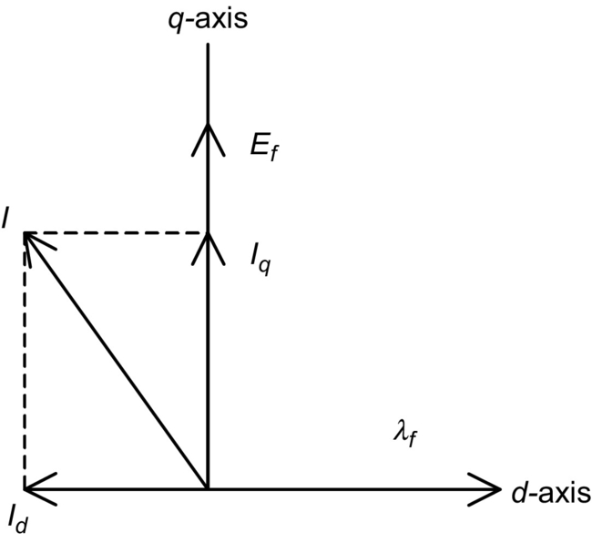
λ′f=λf+LdId
where Id is negative when I leads Ef. If the air gap is small, the d-axis component of the armature current may reduce the rotor flux to the required extent.
30.4.6 Operating Modes
A synchronous motor may be driven with a view to achieving various operating characteristics, such as power factor compensation, maximum torque per ampere characteristic, and field weakening. The power factor at which a synchronous motor operates is an important issue, especially for a large drive. A large angle θ between the input voltage and current phasors of the motor results in a poor overall power factor. The operation of the synchronous motor with stator current waveforms with a certain phase angle with respect to the respective phase back-emf waveforms allows interesting power-factor compensation possibilities. Consider the following three cases.
30.4.6.1 Case 1: Operation with I Lagging Ef
In this case, the motor is underexcited and I lags Ef, by an angle γ, as indicated in Fig. 30.39. The overall power factor in this case is lagging, since I lags V by an angle θ. The power-factor angle θ is larger than γ. Note that Id now magnetizes the rotor field.
30.4.6.2 Case 2: I is in phase with Ef; Maximum Torque per Ampere Operation (γ=0° )
)
If γ=0°![]() is used, the motor input current ia is in phase with the back emf ea, as indicated in the waveforms of Fig. 30.40A. From Eq. (30.65), the developed torque is given by
is used, the motor input current ia is in phase with the back emf ea, as indicated in the waveforms of Fig. 30.40A. From Eq. (30.65), the developed torque is given by
T=KϕI
Thus, for a fixed rotor excitation, the developed torque is the highest that can be achieved per ampere of stator current I. In other words, if γ=0°![]() is chosen, the drive operates with its maximum torque per ampere characteristic. From the phasor diagram of Fig. 30.40B, it is clear that the input current I phasor now lags the voltage V phasor at the motor terminals (see the phasor diagram in the figure). Note that the level of Ef that is determined by the level of excitation also determines the angle θ to some extent. Clearly, when maximum-torque-per-ampere characteristic is required, a power factor less than unity has to be accepted.
is chosen, the drive operates with its maximum torque per ampere characteristic. From the phasor diagram of Fig. 30.40B, it is clear that the input current I phasor now lags the voltage V phasor at the motor terminals (see the phasor diagram in the figure). Note that the level of Ef that is determined by the level of excitation also determines the angle θ to some extent. Clearly, when maximum-torque-per-ampere characteristic is required, a power factor less than unity has to be accepted.
30.4.6.3 Case 3: Operation with I Leading Ef
If I is chosen to lead Ef, the overall power factor can be higher, including unity, as is indicated in Fig. 30.41. Note that the motor now operates with less than maximum torque per ampere characteristic. Note also that the d-axis component of I now tends to demagnetize the rotor and that the operation with field weakening is implied.

With a CSI-driven motor, the amplitude and the angle of the phase current relative to the back emf can be selected according to one of the desirable operating characteristics mentioned above. Additionally, other operational limits such as the inverter/motor-current limit, the maximum stator voltage limit, and the maximum power limit can also be addressed. The amplitude of the stator current I clearly determines the developed torque of the motor. Consequently, the error of the speed controller is used to determine the amplitude of I. The overall control system with an inner torque loop can be described by Fig. 30.42.

30.4.7 Vector Control
Controls described in foregoing sections were based on the steady-state equivalent circuit of the motor. Even though the torque Eq. (30.65) for a current-source drive evokes vector-control-like relationships, they do not address the dynamics of the current controls as is possible in an orthogonal reference frame. Using an orthogonal set of reference attached to the rotor, a simple set of decoupled, dc-motor-like torque-control relationships is readily obtained. Following the transformation technique used in Section 30.3.4, the stator voltage equations of a synchronous motor with fixed rotor excitation in the rotor reference frame are
[vqvd]=[R+pLqωLd−ωLqR+pLd][iqid]+[ωλf0]

T=32P(λfiq+(Ld−Lq)idiq)
where all the quantities in lower case represent instantaneous quantities in the rotor dq-frame. The λf is the flux linkage per phase due to the rotor excitation, ω is the electric angular velocity in radians per second, and P is the number of pole pairs. Here, p is the time derivative operator d/dt. Assuming the magnetic linearity, the stator flux linkages are
λd=Ldid+λfλq=Lqiq

Note that the Eq. (30.68) can be written down directly from Eq. (30.31), taking into account the fixed rotor excitation so that the third and fourth rows and columns of Eq. (30.31) may be dropped. Since the reference frame now rotates at the speed of the rotor, ωe=ω![]() . The induced back emf due to the fixed rotor excitation occurs in the rotor q-axis and is included in Eq. (30.68), as a separate term. Similarly, the torque expression of Eq. (30.69) may also be written down from Eq. (30.41), using the flux linkages of Eq. (30.70).
. The induced back emf due to the fixed rotor excitation occurs in the rotor q-axis and is included in Eq. (30.68), as a separate term. Similarly, the torque expression of Eq. (30.69) may also be written down from Eq. (30.41), using the flux linkages of Eq. (30.70).
Eqs. (30.67)–(30.69) are for a salient-pole motor for which Ld≠Lq![]() . For a nonsalient-pole motor, Ld is equal to Lq, and the developed torque is proportional to iq only. In either case, the inner torque loop consist of two separate current loops: one for id and the other for iq, as indicated in Fig. 30.43. The iq current loop generally derives its reference signal from the output of the speed controller and constitutes the inner torque loop. The reference for the id current loop is normally specified by the extent of field weakening for which a negative id reference is used. Otherwise, the d-axis current is maintained at zero. Note that for large synchronous motors with variable external excitation, field weakening is normally applied through adjustment of the rotor excitation, using a spillover signal from the output of the speed controller.
. For a nonsalient-pole motor, Ld is equal to Lq, and the developed torque is proportional to iq only. In either case, the inner torque loop consist of two separate current loops: one for id and the other for iq, as indicated in Fig. 30.43. The iq current loop generally derives its reference signal from the output of the speed controller and constitutes the inner torque loop. The reference for the id current loop is normally specified by the extent of field weakening for which a negative id reference is used. Otherwise, the d-axis current is maintained at zero. Note that for large synchronous motors with variable external excitation, field weakening is normally applied through adjustment of the rotor excitation, using a spillover signal from the output of the speed controller.

From Eq. (30.68), it is clear that the couplings of q- and d-axis voltages exist through the d- and q-axis currents, respectively, and the back emf. During dynamic operation, such coupling effects become undesirable. The coupling effects of d- and q-axis currents and the back emf into q- and d-axis voltages, respectively, can be removed by the feedforward terms shown in the shaded part of the block the diagram of Fig. 30.44, which also shows the two current-control loops. The two outputs v∗d![]() and v∗q
and v∗q![]() from the decoupled current controllers are transformed to the stator reference frame before being subjected to pulse-width modulators or hysteresis comparators. Note that the current references i∗d
from the decoupled current controllers are transformed to the stator reference frame before being subjected to pulse-width modulators or hysteresis comparators. Note that the current references i∗d![]() and i∗q
and i∗q![]() are obtained with due regard for the desired operating and limiting conditions as described in Section 30.4.5.
are obtained with due regard for the desired operating and limiting conditions as described in Section 30.4.5.

Under this type of control, which is exercised in the rotor reference frame, the d- and q-axis currents are separately regulated. The purpose of the q-axis current controller is primarily to control the developed torque, especially for the nonsalient-pole motor. For this motor, the d-axis current is normally maintained at zero, when the motor is operated below the base speed. The d-axis current may be used to weaken the air-gap flux so that the motor operates with a constant-power-like characteristic. It should be noted that the field weakening may also be carried out more directly by adjusting the rotor excitation current by using a spillover signal from the speed controller, when the base speed is exceeded.
The dynamic response of the drive under the vector control scheme indicated in Fig. 30.44 is the highest possible with a CSI drive. It should also be noted that the dq currents in the rotor reference frame vary only the mechanical dynamics of the rotor. In fact, they are dc quantities when the motor runs at a constant speed. Consequently, the following error (or lag) associated with tracking a sinusoidally time-varying current reference, which is the case when current control is exercised in the stator a−b−c![]() reference frame, can be reduced easily by using an integral-type current controllers.
reference frame, can be reduced easily by using an integral-type current controllers.
30.5 Permanent-Magnet Synchronous Motor Drives
30.5.1 Introduction
Since the introduction of samarium cobalt and neodymium-iron-boron magnetic materials in the 1970s and 1980s, respectively, synchronous motors with permanent-magnet excitation in the rotor have been displacing the dc motor in many high-performance applications. The trend is more noticeable in applications requiring high-performance motors of up to a few kilowatts. In low- to medium-power applications, the superior dynamics, smaller size, and higher efficiency of motors with PM excitation in the rotor, compared with all other motors, are well-known.
The arrangement just mentioned is very similar to a conventional synchronous motor. This is particularly so when the stator windings and the rotor mmf are sinusoidally distributed. Several rotor configurations of the PM synchronous motor have been developed, of which the important ones are indicated in Figs. 30.45–30.47.


30.5.2 The Surface-Magnet Synchronous Motor with Trapezoidal Back Emf Waveform
The surface-magnet motor comes with the rotor magnets glued onto the surface of the rotor. An additional stainless steel (i.e., nonmagnetic) cylindrical shell may be used to cover the rotor in order to keep the magnets in place against centrifugal force in high-speed applications. Since the relative permeability of the magnetic material is very close to unity, the effective air gap is uniform and large. Because the air gap includes the magnet thickness, it is long. Consequently, the synchronous inductances along the rotor d- and q-axes, as indicated in Fig. 30.45, are equal and small (i.e., Ld=Lq=Ls![]() ). The armature reaction in this type of motor is small.
). The armature reaction in this type of motor is small.
The three-phase winding in the stator has uniformly distributed windings. The span of the magnets are selected in such a way that the back emf induced in the stator windings are trapezoidal with nearly 120° of constant amplitude in each half cycle. Such a motor, often called a brushless dc (BLDC) motor because of its similarity to the inside-out conventional brushed PM DC motor, develops a trapezoidal back-emf waveform as indicated in Fig. 30.48, when it is driven at a constant speed. The back-emf waveforms have flattops for nearly 120° in each half cycle followed by 60° of transition from positive to negative polarity of voltage and vice versa. These motors are very suitable for variable-speed applications such as spindle drives in machine-tool and disk drives.

30.5.2.1 Control of the Trapezoidal-wave Motor
Neglecting higher-order harmonic terms, the back emf in the motor phases may be as indicated in Fig. 30.49. Each back emf has a constant amplitude (or flattop) for 120° (electric) followed by 60° of transition in each half cycle. The developed torque at any instant is given by
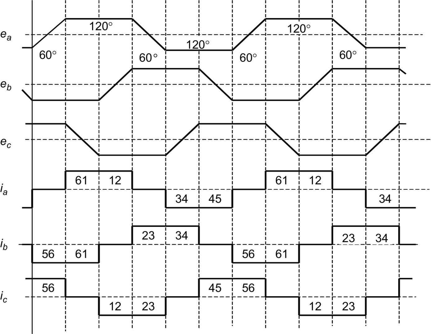
T=eania+ebnib+ecnicωNm
It is readily seen that the ideal current waveform in each phase needs to be a quasi-square waveform of 120° of conduction angle in each half cycle. The conduction of current in each phase winding coincides with the flat part of the back-emf waveforms, which guarantees that the developed torque, that is, (c∑x=aexn⋅ixnωr) , is constant or ripple-free at all times. With such quasi-square current waveforms, a simple set of six optocouplers or Hall-effect sensors would be required to drive the six inverter switches indicated in Fig. 30.36. The output current waveforms for the three-phase inverter and the switching devices that conduct during the six switching intervals per cycle are also indicated in Fig. 30.49. Since only six discrete outputs per electric cycle are required from the rotor-position sensors, the requirement of a high-resolution position sensor is dispensed with. Continuous current control for each phase of the motor, by hysteresis or PWM control, to regulate the amplitude of the motor current in each phase is normally employed. The operation of the BLDC motor drive is further described in detail in Section 30.6.
Even though careful electromagnetic design is employed in order to have perfect trapezoidal back-emf waveforms as indicated in Fig. 30.49, the back-emf waveforms in a practical brushless dc motor exhibit some harmonics, as indicated in Fig. 30.48. If ripples in the back-emf waveforms are significant, then torque ripples will also exist when the motor is driven with quasi-square phase current waveforms. These ripples may become troublesome when the motor is operated at a low speed, when the motor load inertia may not filter out the torque ripples adequately.
A second source of torque ripple in the permanent-magnet brushless dc (PM BLDC) motor is from the commutation of current in the inverter. Since the actual phase currents cannot have the abrupt rise and fall times as indicated in Fig. 30.49, torque spikes, one for each switching, may exist.
Even though the PM BLDC motor does not have sinusoidal back emf and inductance variations with rotor angle, the analysis of Section 30.4 in terms of the fundamental quantities will often suffice. The switching of the inverter using the six rotor-position sensors guarantees that the current waveform in each phase always remains in synchronism with the back emf of the respective phase. Since the quasi-square phase current waveform in each phase coincides with the flat part of the back-emf waveform of the same phase, the angle γ is clearly zero for such operation. Thus, considering fundamental quantities, the motor back emf and the torque characteristics can be expressed by
E=KEωV
T=KTIcosγ=KTINm
where KE and KT are equal in consistent units. Note that E and I are now RMS values of the fundamental components of these quantities.
30.5.2.2 Sensorless Operation of the PM BLDC Motor
In spindle and other variable-speed drive applications, where the lowest speed of operation is not less than a few hundred revolutions per minute, it is possible to obtain the switching signals for the inverter from the motor back emf, thus dispensing with rotor-position sensors. The method consists of integrating the back-emf waveforms, which are the same as the applied phase voltage if the other voltage drops are neglected, and comparing the integrated outputs with a fixed reference. These comparator outputs determine the switching signals for inverter. It may be noted that the amplitude of the back-emf waveforms is proportional to the operating speed, so that the frequency of the comparator outputs increases automatically with speed. In other words, the angle γ and the current waveform relative to the back-emf waveform in each phase remains the same regardless of the operating speed. Integrated circuits are available from several suppliers that perform this task of sensorless BLDC operation satisfactorily, covering a reasonable speed range.
30.5.3 The PM Synchronous Motor with Sinewave Back Emf Waveforms
The PM sine-wave motor, which may also have magnets on the rotor surface or buried inside the rotor (as in the interior-magnet motor of Fig. 30.46), typically has sinusoidally distributed windings. The air-gap flux distribution produced by the rotor magnets is also sinusoidal, arranged through magnet and rotor flux barrier shaping. Consequently, the back-emf waveform of each phase when running at a constant speed is also a sinusoidal waveform, as indicated in Fig. 30.50, when the motor is driven at a constant speed.
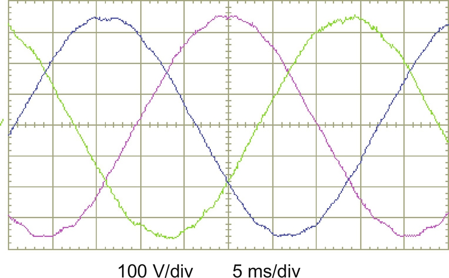
 .
.It should be noted, however, that with magnets mounted on the rotor surface, the effective air gap is large and uniform so that Ld=Lq=Ls![]() . Because of the large equivalent air gap, these inductances are also small, and consequently, the armature reaction is small. As a result, this motor essentially operates with fixed excitation, and there is hardly any scope for altering the operating power factor or the rotor mmf, once the motor and its drive voltage and current ratings have been selected.
. Because of the large equivalent air gap, these inductances are also small, and consequently, the armature reaction is small. As a result, this motor essentially operates with fixed excitation, and there is hardly any scope for altering the operating power factor or the rotor mmf, once the motor and its drive voltage and current ratings have been selected.
The interior permanent-magnet synchronous motor (IPMSM), which comes with magnets buried inside the rotor as indicated in Figs. 30.46, has an easier magnetization path along the rotor q-axis, so that Lq>Ld![]() . The small air gap implies that the inductances Ld and Lq may not be small and hence may allow considerable scope for field weakening.
. The small air gap implies that the inductances Ld and Lq may not be small and hence may allow considerable scope for field weakening.
If the sine-wave motor is supplied from an PWM inverter, the analyses and vector diagrams of PM sine-wave motor are similar to those in Section 30.4 for the nonsalient-pole and salient-pole synchronous motor drives. The surface-magnet motor is more akin to the nonsalient-pole motor, since Ld=Lq=Ls![]() , whereas the interior-magnet motor is more akin to the salient-pole motor because of the d- and q-axis inductances being unequal. Thus, the equations in Section 30.4 will apply equally well for this motor, both in the steady state and dynamically and for both voltage- and current-source supply.
, whereas the interior-magnet motor is more akin to the salient-pole motor because of the d- and q-axis inductances being unequal. Thus, the equations in Section 30.4 will apply equally well for this motor, both in the steady state and dynamically and for both voltage- and current-source supply.
30.5.3.1 Control of the PM Sinewave Motor
The sinusoidal back-emf waveforms imply that the three-phase motor must be supplied with a sinusoidal three-phase current if a dc-motor-like (or vector-control-like) torque characteristic is desired, as was found in Section 30.4. For such operation, the phase currents must also be synchronized with the respective phase back-emf waveforms, in other words, with the rotor dq- reference frame. This implies the operation with a specified γ angle. Two implementations are possible.
In one scheme, the stator currents are regulated in the stator reference frame, and the stator current references are produced with reference to the rotor position, as indicated in Fig. 30.51. The rotor position θ is continuously sensed and used to produce three sinusoidal current references of unit amplitude. The phase angle γ of the references relative to the respective back-emf waveforms is usually derived from the speed controller, which defines the field-weakening regime of the drive. The operating power factor of the drive may also be addressed using the γ angle control, as explained in Section 30.4.5. The amplitudes of these references are then multiplied by the error of the speed controller in order to produce the desired torque reference. In this way, both the RMS value I of the phase current and its angle γ with respect to Ef can be adjusted independently (which is equivalent to independent dq-axis current control). Three PWM current controllers are indicated, but two suffice for a balanced motor. Other types of current controllers, such as hysteresis controllers, may also be used.

In the second scheme, the motor currents are first transformed into the rotor dq-reference frame using continuous rotor-position feedback, and the measured rotor d- and q-axis currents are then regulated in the rotor reference frame, as indicated in Fig. 30.52. The main advantage of regulating the stator currents in the rotor reference frame, compared with the stator reference frame as in the first scheme, is that current references now vary more slowly and hence suffer from lower tracking error. At constant speed, the stator current references are in fact dc quantities as opposed to ac quantities, and hence, the inevitable tracking errors of the former scheme are easily removed by an integral-type controller. The other advantage is that the current references may now include feedforward decoupling so as to remove the cross coupling of the d- and q-axis variables as shown in the motor representation of Fig. 30.52. The latter scheme is currently preferred, since it allows more direct control of the currents in the rotor reference frame.

It should be noted that continuous transformations to and from rotor dq-axes are required; hence, the rotor-position sensor is a mandatory requirement. Rotor-position sensors of 10- to 12-bit accuracy are normally required. This is generally viewed as a weakness for this type of drive.
The general torque relationship of a sine-wave motor supplied from a current-source SPWM inverter is given by Eq. (30.69) that is rewritten here:
T=32P(λfiq+(Ld−Lq)idiq)
Precise control of the developed torque control requires that both id and iq be actively controlled in order to regulate it to the level determined by the error of the speed controller. For the surface-magnet synchronous motor, the large effective air gap means that Ld≈Lq![]() , so that id should be maintained at zero level. This implies that the id current reference in Fig. 30.52 should be kept zero. For the interior-magnet motor, Lq>Ld
, so that id should be maintained at zero level. This implies that the id current reference in Fig. 30.52 should be kept zero. For the interior-magnet motor, Lq>Ld![]() , so that id and iq have to be controlled simultaneously to develop the desired torque. A few modes of operation are possible.
, so that id and iq have to be controlled simultaneously to develop the desired torque. A few modes of operation are possible.
30.5.3.2 Operating Modes
Operation with maximum torque per ampere (MTPA) characteristic
In this mode of control, the developed torque T per ampere of stator current is the highest for a given rotor excitation. The combination of id and iq that develops the maximum torque per ampere of stator current is indicated in Fig. 30.53. The reference signal for the inner torque loop normally determines the iq reference, while the id reference is given by
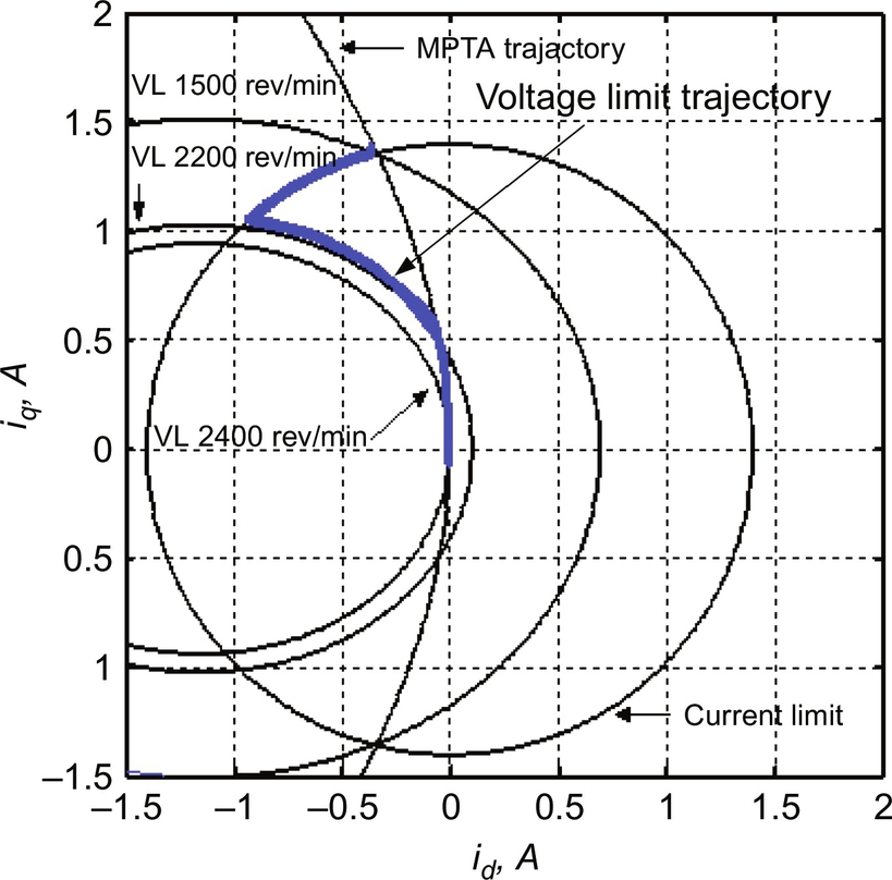
 Trajectories for the maximum torque per ampere characteristic and for maximum voltage and current limits of an interior PM motor.
id=λf2(Lq−Ld)−√λ2f4(Lq−Ld)2+i2q
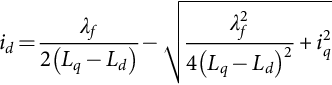
It should be noted that with id=0![]() , this mode of operation is achieved for the surface-magnet motor.
, this mode of operation is achieved for the surface-magnet motor.
Operation with voltage and current limits
The maximum current limit of the motor/inverter, Ismax, is normally imposed by setting appropriate limits on id and iq such that
i2d+i2q≤I2smax
Eq. (30.75) defines a circle around the origin of the id−iq![]() plane.
plane.
The available dc-link voltage to the inverter places an upper limit of the motor phase voltage, Vsmax, given by
V2=V2d+V2q≤V2max
(Lqiq)2+(Ldid+λf)2≤(Vamω)2

where the stator voltages vd and vq are expressed in the rotor reference frame, as in Eq. (30.68). Eq. (30.78) is obtained from the voltage equation of Eq. (30.68) when the phase resistance R is neglected. Eq. (30.78) defines elliptical trajectories that contract as speed increases. All the three modes of operation are included in Fig. 30.53.
Operation with field weakening
This mode of operation is normally required for operating the motor above the base speed. A constant-power characteristic is normally desired over the full field-weakening range. For a given rotor excitation of λf and developed power of P0, the developed torque T and the net rotor flux linkage required for constant-power operation can be determined. From this, the limiting values for id and iq, which further constrain the allowable id−iq![]() trajectory is also indicated in Fig. 30.53, can be determined.
trajectory is also indicated in Fig. 30.53, can be determined.
The operating modes described in the preceding section are normally included in a trajectory controller that generates the references for id and iq continuously, as indicated in Fig. 30.54.