
HVDC Transmission
Vijay K. Sood University of Ontario Institute of Technology, Oshawa, ON, Canada
Abstract
High-voltage direct current (HVDC) is a mature technology and a large user of power electronics technology. from its humble beginning with mercury-arc valves in 1954 with an undersea inter-connection to the island of Gotland, it has now become a major technology transporting bulk power over long distances and inter-connecting asynchronous AC systems. This chapter presents the theoretical background of the original line-commutated convertors to the voltage source converters implemented with the latest transistor technology.
Keywords
HVDC transmission; Line-commutated converters; Voltage-source converters; DC transmission line
Abbreviations
AEP American Electric Power
ASVC Advanced static var compensator
BB Back to back
BC Hydro British Columbia Hydro
BESS Battery energy storage system
BPA Bonneville Power Authority
CCC Capacitor-commutated converter
CSCC Controlled series capacitor-commutated converter
EMTP Electromagnetic transient program
EPRI Electric Power Research Institute
FACTS Flexible AC transmission system
GTO Gate turn off (thyristor)
HVDC High-voltage direct current
IEE Institute of Electrical Engineers
IEEE Institute of Electrical and Electronic Engineers
IGBT Insulated-gate bipolar transistor
IPC Interphase power controller
LT Load tap
MP Minnesota Power
MSC Mechanical switch controller
NSP Northern States Power Co.
PLL Phase-locked loop
PSS Power system stabilizer
PWM Pulse-width modulation
SMES Superconducting magnetic energy storage
SSR Subsynchronous resonance
STATCON Static condenser
STATCOM Static compensator
SVC Static var compensator
TCBR Thyristor-controlled braking resistor
TCPAR Thyristor-controlled phase-angle regulator
TCSC Thyristor-controlled switched capacitor
TNA Transient network analyzer
TSC Thyristor-switched capacitor
TSR Thyristor-switched reactor
TVA Tennessee Valley Authority
UPFC Unified power flow controller
VSI Voltage-source inverter
WAPA Western Area Power Authority
Acknowledgments
The author pays tribute to the many pioneers whose vision of HVDC transmission has led to the rapid evolution of the power industry. It is not possible here to name all of them individually.
A number of photographs of equipment have been included in this chapter, and I thank the suppliers (Mr. P. Lips of Siemens and Mr. R. L. Vaughan from ABB) for their assistance in getting clearances.
I also thank my wife Vinay for her considerable assistance in the preparation of this manuscript.
27.1 Introduction
High-voltage direct current (HVDC) transmission [1–3] is a major user of power electronics technology. HVDC technology first made its mark in the early undersea cable interconnections of Gotland (1954) and Sardinia (1967) and then in long-distance transmission with the Pacific Intertie (1970) and Nelson River (1973) schemes using mercury-arc valves. A significant milestone development occurred in 1972 with the first back-to-back (BB) asynchronous interconnection at Eel River between Quebec and New Brunswick; this installation also marked the introduction of thyristor valves to the technology and replaced the earlier mercury-arc valves.
Until 2005, a total of 70,000 MW HVDC transmission capacity is installed in some 95 projects all over the world. To understand the rapid growth of DC transmission (Table 27.1) [4] in the past 50 years, it is first necessary to compare it to conventional AC transmission.
Table 27.1
Listing of HVDC installations
| HVDC link | Supplier | Year | Power MW | DC Voltage kV | Length km | Location |
| Gotland Ia | A | 1954 | 20 | ±100 | 96 | Sweden |
| English Channel | A | 1961 | 160 | ±100 | 64 | England-France |
| Volgograd-Donbassb | 1965 | 720 | ±400 | 470 | Russia | |
| Inter-Island | A | 1965 | 600 | ±250 | 609 | New Zealand |
| Konti-Skan I | A | 1965 | 250 | 250 | 180 | Denmark-Sweden |
| Sakuma | A | 1965 | 300 | 2×125 | B-Bc | Japan |
| Sardinia | I | 1967 | 200 | 200 | 413 | Italy |
| Vancouver I | A | 1968 | 312 | 260 | 69 | Canada |
| Pacific Intertie | JV | 1970 | 1440 | ±400 | 1362 | The United States |
| Pacific Intertie | 1982 | 1600 | ||||
| Nelson River Id | I | 1972 | 1620 | ±450 | 892 | Canada |
| Kingsnorth | I | 1975 | 640 | ±260 | 82 | England |
| Gotland | A | 1970 | 30 | ±150 | 96 | Sweden |
| Eel River | C | 1972 | 320 | 2×80 | B-B | Canada |
| Skagerrak I | A | 1976 | 250 | 250 | 240 | Norway-Denmark |
| Skagerrak II | A | 1977 | 500 | ±250 | Norway-Denmark | |
| Skagerrak III | A | 1993 | 440 | 350 | 240 | Norway-Denmark |
| Vancouver II | C | 1977 | 370 | −280 | 77 | Canada |
| Shin Shinano | D | 1977 | 300 | 2×125 | B-B | Japan |
| Shin Shinano | 1992 | 600 | 3×125 | B-B | Japan | |
| Square Butte | C | 1977 | 500 | ±250 | 749 | The United States |
| David A. Hamil | C | 1977 | 100 | 50 | B-B | The United States |
| Cahora Bassa | J | 1978 | 1920 | ±533 | 1360 | Mozambique-S. Africa |
| Nelson River II | J | 1978 | 900 | ±250 | 930 | Canada |
| Nelson River II | J | 1985 | 1800 | ±500 | 930 | Canada |
| CU Project | A | 1979 | 1000 | ±400 | 710 | The United States |
| Hokkaido-Honshu | E | 1979 1980 1993 |
150 300 600 |
125 250 ±250 |
168 | Japan |
| Acaray | G | 1981 | 50 | 25.6 | B-B | Paraguay |
| Vyborg Vyborg Vyborg |
F F F |
1981 1982 |
355 710 1065 |
1×170(±85) 2×170 3×170 |
B-B | Russia (tie with Finland) |
| Duernrohr | J | 1983 | 550 | 145 | B-B | Austria |
| Gotland II | A | 1983 | 130 | 150 | 100 | Sweden |
| Gotland III | A | 1987 | 260 | ±150 | 103 | Sweden |
| Eddy County | C | 1983 | 200 | 82 | B-B | The United States |
| Châteauguay | J | 1984 | 1000 | 2×140 | B-B | Canada |
| Oklaunion | C | 1984 | 200 | 82 | B-B | The United States |
| Itaipu | A | 1984 | 1575 | ±300 | 785 | Brazil |
| Itaipu | A | 1985 | 2383 | 785 | Brazil | |
| Itaipu | A | 1986 | 3150 | ±600 | 785 | Brazil |
| Inga-Shaba | A | 1982 | 560 | ±500 | 1700 | DR Congo |
| Pacific Intertie upgrade | A | 1984 | 2000 | ±500 | 1362 | The United States |
| Blackwater | B | 1985 | 200 | 57 | B-B | The United States |
| Highgate | A | 1985 | 200 | ±56 | B-B | The Unite States |
| Madawaska | C | 1985 | 350 | 140 | B-B | Canada |
| Miles City | C | 1985 | 200 | ±82 | B-B | The United States |
| Broken Hill | A | 1986 | 40 | 2×17(±8.33) | B-B | Australia |
| Intermountain Power Project | A | 1986 | 1920 | ±500 | 784 | The United States |
| Cross-Channel: Les Mandarins (Sellindge) |
H I |
1986 1986 |
1000 2000 |
±270 2×±270 |
72 | France-England France England |
| Des Cantons-Comerford | C | 1986 | 690 | ±450 | 172 | Canada-the United States |
| Sacoie Sacoif |
H H |
1986 1992 |
200 300 |
200 | 415 | Corsica Island Italy |
| Itaipu II | A | 1987 | 3150 | ±600 | 805 | Brazil |
| Sidney (Virginia Smith) | G | 1988 | 200 | 55.5 | B-B | The United States |
| Gezhouba-Shanghai | B+G | 1989 1990 |
600 1200 |
500 ±500 |
1000 | China |
| Konti-Skan II | A | 1988 | 300 | 285 | 150 | Sweden-Denmark |
| Vindhyachal | A | 1989 | 500 | 2×69.7 | B-B | India |
| Pacific Intertie Exp. | B | 1989 | 1100 | ±500 | 1362 | The United States |
| McNeill | I | 1989 | 150 | 42 | B-B | Canada |
| Fenno-Skan | A | 1989 | 500 | 400 | 200 | Finland-Sweden |
| Sileru-Barsoor | K | 1989 | 100 200 400 |
+100 +200 ±200 |
196 | India |
| Rihand-Delhi | A | 1991 | 1500 | ±500 | India | |
| Quebec-New England Nicolet Tap |
A A |
1990 1992 |
2000g 1800 |
±450 | 1500 | Canada-the United States Canada |
| DC Hybrid Link | AB | 1992 | 992 | +270/−350 | 617 | New Zealand |
| Etzenricht | G | 1993 | 600 | 160 | B-B | Germany (tie with Czech) |
| Vienna Southeast | G | 1993 | 600 | 145 | B-B | Austria (tie with Hungary) |
| Haenam-Cheju | I | 1993 | 300 | ±180 | 100 | South Korea |
| Baltic Cable Project | AB | 1994 | 600 | 450 | Sweden-Germany | |
| Welch-Monticello | 1995 | 600 | B-B | The United States | ||
| Kontek Interconnection | 1995 | 600 | 400 | 170 | Denmark-Germany | |
| Scotland-N. Ireland | 1996 | 250 | 250 | The United Kingdom | ||
| Chandrapur-Ramagundum | 1996 | 1000 | 2×500 | B-B | India | |
| Chandrapur-Padghe | AB | 1997 | 1500 | ±500 | 900 | India |
| Greece-Italy | AB | 1997 | 500 | 400 | 200, sea | Italy |
| Gajuwaka-Jeypore | AB | 1997 | 500 | B-B | India | |
| Leyte-Luzon | AB | 1997 | 1600 | 400 | 440 | Philippines |
| Cahora Bassa | G | 1998 | 1920 | ±533 | 1456 | Mozambique-S. Africa |
| TSQ-Beijao | G | 2000 | 1800 | ±500 | 903 | China |
| Thailand-Malaysia | G | 2001 | 300 | ±300 | B-B | Thailand-Malaysia |
| Moyle | G | 2001 | 2×250 | 250 | 64 | Ireland-Scotland |
| East-South Intercon. | G | 2003 | 2000 | ±500 | 1450 | India |
| Rapid City DC tie | AB | 2003 | 2×100 | ±13 | B-B | S. Dakota, the United States |
| Three Gorges-Changzhou | AB | 2003 | 3000 | ±500 | 890 | China |
| Three Gorges-Guangdong | AB | 2004 | 3000 | ±500 | 940 | China |
| Guizhou-Guangdong | G | 2004 | 3000 | ±500 | 940 | China |
| Celilo conv. station | AB | 2004 | 2000 | ±500 | Upgrade | The United States |
| Nelson River Bipole II | G | 2004 | 1000 | 450 | Pole 1 | Canada |
| Basslink | G | 2005 | 500 | 400 | 350 | Australia-Tasmania |
| Lamar | G | 2005 | 210 | 63.6 | B-B | Colorado, the United States |
| Vizag II | AB | 2005 | 500 | ±88 | B-B | India |
| Estlink | AB | 2006 | 350 | ±150 | HVDC Light | Estonia-Finland |
| Three Gorges-Shanghai | AB | 2007 | 3000 | ±500 | 1059 | China |
| NorNed | AB | 2007 | 700 | ±450 | 560 | Norway-Netherlands |
| Valhall offshore | AB | 2009 | 950 | HVDC Light | Norway | |
| Yunnan-Guangdong | G | 2009 | 5000 | ±800 | 1418 | China |
| Outaouais | AB | 2009 | 1250 | 175 | B-B | Canada |
| Blackwater | AB | 2009 | 200 | 57 | B-B | The United States |
| Ballia-Bhiwadi | G | 2010 | 2500 | ±500 | 800 | India |
| Storebælt | G | 2010 | 600 | 400 | 56 | Denmark |
| Trans Bay Cable project | G | 2010 | 400 | ±200 | 85 | The United States |
| Hulunbeir-Liaoning | AB | 2010 | 3000 | ±500 | 920 | China |
| Xiangjiaba-Shanghai | G | 2010 | 6400 | ±800 | 2070 | China |
| Caprivi Link | AB | 2010 | 300 | 350 | 950 | Namibia |
| Intermountain Power | AB | 2010 | 2400 | ±500 | 785 | The United States |
| Lingbao II | AB | 2010 | 750 | 168 | B-B | Chain |
| BritNed, Great Britain | G | 2011 | 1000 | ±450 | 260 | Netherlands |
| SAPEI | AB | 2011 | 1000 | ±500 | 2×450 | Italy-Sardinia |
| Fenno-Skan | AB | 2011 | 500 | 400 | 200 | Finland-Sweden |
| Valhall | AB | 2011 | 78 | 150 | 292 | Norway |
| COMETA | G | 2012 | 2×200 | ±200 | 250 | Spain |
| Jinping-Sunan | G | 2012 | 7200 | ±800 | 2059 | China |
| Mundra-Haryana | G | 2012 | 2500 | ±500 | 960 | India |
| Highgate | AB | 2012 | 200 | 57 | B-B | Canada |
| Back to back | G | 2013 | 500 | 158 | B-B | Bangladesh |
| Porto Velho | AB | 2013 | 2×400 | ? | B-B | Brazil |
| Black Sea Transmission | G | 2013 | 2×350 | 96 | B-B | Georgia |
| Hudson Transmission | G | 2013 | 660 | 180 | B-B | The United States |
| East-West Interconnector | AB | 2013 | 500 | ±200 | 2×75 | The United Kingdom-Ireland |
| Jinping-Sunan | AB | 2013 | 7200 | ±800 | 2090 | China |
| Nuozhadu-Guangdong | G | 2013 | 5000 | ±800 | 1451 | China |
| Rio Madeira | AB | 2013 | 2×400 | ±600 | B-B | Brazil |
| Xiluodu-Guangdong | G | 2013 | 6400 | ±500 | 1286 | China |
| INELFE | G | 2014 | 2×1000 | ±320 | 65 | France-Spain |
| Mackinac | AB | 2014 | 200 | ±71 | B-B | The United States |
| Inga-Kolwezi | AB | 2014 | 560 | ±500 | 1700 | Congo |
| Skagerrak | AB | 2014 | 700 | 500 | 140 | Norway-Denmark |
| Eel River | AB | 2014 | 350 | 80 | B-B | Canada |
| EstLink 2 | G | 2014 | 670 | 450 | 171 | Finland-Estonia |
| Railroad DC Tie | AB | 2014 | 300 | ±21 | B-B | Mexico |
| Oklaunion | AB | 2014 | 220 | ±31 | B-B | The United States |
| Inter-Island Connector Pole 3 | G | 2014 | 700 | ±350 | 649 | New Zealand |
| Western HVDC Link | G | 2015 | 2200 | ±600 | 420 | The United Kingdom |
| Troll A 3&4 | AB | 2015 | 100 | ±60 | 70 | Norway |
| DolWin1 | AB | 2015 | 800 | ±320 | 2×75 | Germany |
| ÅL-link | AB | 2015 | 100 | ±80 | 158 | Finland |
| BorWin1 | AB | 2015 | 400 | ±150 | 2×75 | Germany |
| LitPol Link | AB | 2015 | 500 | ±60 | B-B | Poland-South Lithuania |
| Madawaska | AB | 2016 | 350 | 130 | B-B | Canada |
| Pacific Intertie | AB | 2016 | 1440 | ±400 | 1360 | The United States |
| NordBalt | AB | 2016 | 700 | ±320 | 400 | Sweden-Lithuania |
| DolWin2 | AB | 2016 | 916 | ±320 | 2×45 | Germany (North Sea) |
| North-East Agra | AB | 2016 | 6000 | ±800 | 1728 | India |
| Québec-New England | AB | 2016 | 2000 | ±450 | 1480 | Canada-the United States |


A, ASEA; B, Brown Boveri; C, General Electric; D, Toshiba; E, Hitachi; F, Russian; G, Siemens; H, CGEE Alstom; I, GEC (formerly English Electric); J, HVDC W.G. (AEG, BBC, and Siemens); K, (Independent); AB, ASEA Brown Boveri (ABB); JV, Joint Venture (GE and ASEA).
a Retired from service.
b Two VGs replaced with thyristors in 1977.
c Back-to-back HVDC system.
d Two VGs in pole 1 replaced with thyristors by GEC in 1991.
e 50 MW thyristor tap.
f Uprated with thyristor valves.
g Multiterminal system. Largest terminal is rated 2250 MW.
27.1.1 Comparison of AC-DC Transmission
Making a planning selection between either AC or DC transmission is based on an evaluation of transmission costs, technical considerations, and reliability/availability offered by the two power transmission alternatives.
27.1.1.1 Evaluation of Transmission Costs
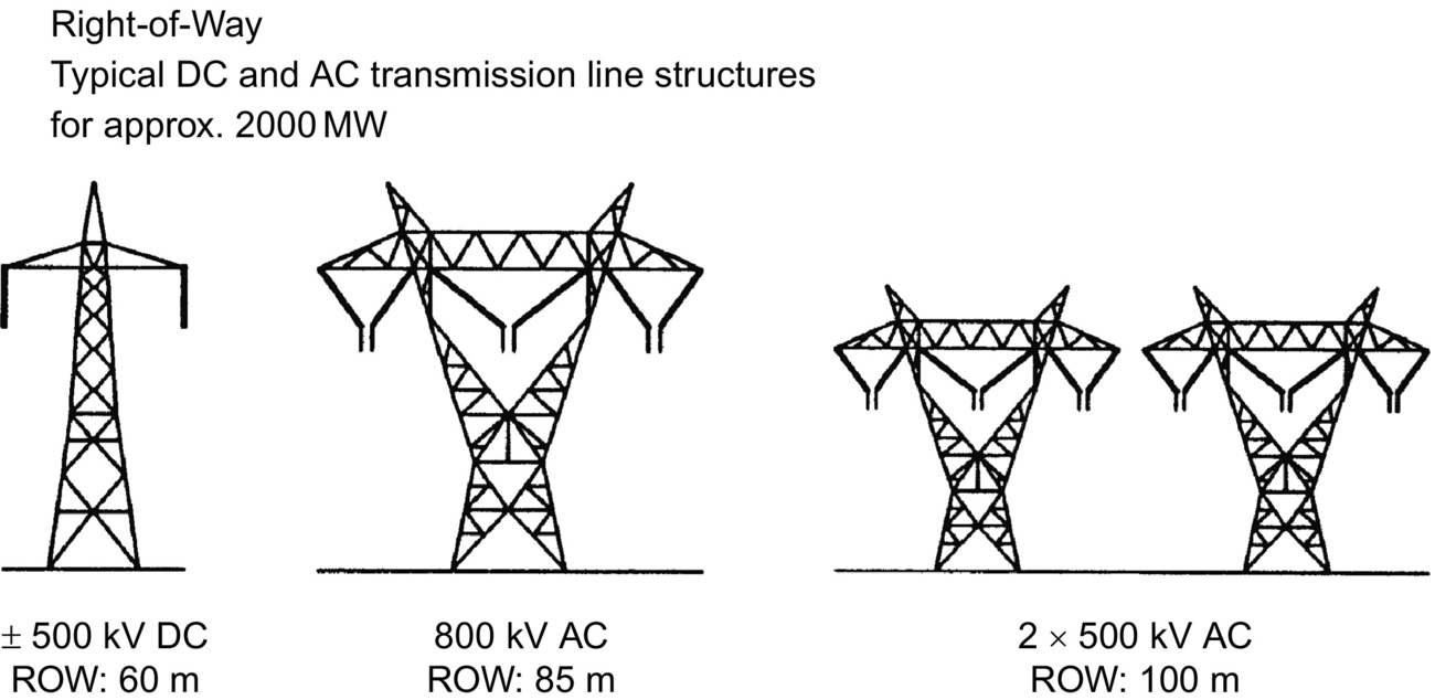
The cost of a transmission line comprises the capital investment required for the actual infrastructure (i.e., right of way (RoW), towers, conductors, insulators, and terminal equipment) and costs incurred for operational requirements (i.e., losses). Assuming similar insulation requirements for peak voltage levels for both AC and DC lines, a DC line can carry as much power with two conductors (having positive/negative polarities with respect to ground) as an AC line with three conductors of the same size. Therefore, for a given power level, a DC line requires a smaller RoW, simpler and cheaper towers, and reduced conductor and insulator costs. As an example, Fig. 27.1 shows the comparative case of AC and DC systems carrying 2000 MW.
With the DC option, since there are only two conductors (with the same current capacity of three AC conductors), the power transmission losses are also reduced to about two-thirds of the comparable AC system. The absence of skin effect with DC is also beneficial in reducing power losses marginally, and the dielectric losses in the case of power cables are also very much less for DC transmission.
Corona effects tend to be less significant on DC than for AC conductors. The other factors that influence line costs are the costs of compensation and terminal equipment. DC lines do not require reactive power compensation, but the terminal equipment costs are increased due to the presence of converters and filters.
Fig. 27.2 shows the variation of infrastructure costs with distance for AC and DC transmission. AC tends to be more economical than DC for distances less than the “break-even distance” but is more expensive for longer distances. This is due to a combination of the terminal equipment costs and line costs for the two types of transmission. The break-even distances can vary from about 500 to 800 km in overhead lines depending on the per unit line costs. With a cable system, this break-even distance approaches 50 km.

27.1.1.2 Evaluation of Technical Considerations
Due to its fast controllability, a DC transmission system has full control over transmitted power, an ability to enhance transient and dynamic stability in associated AC networks and can limit fault currents in the DC lines. Furthermore, DC transmission overcomes some of the following problems associated with AC transmission:
• Stability limits
The power transfer in an AC line is dependent on the angular difference between the voltage phasors at the two line ends. For a given power transfer level, this angle increases with distance. The maximum power transfer is limited by the considerations of steady state and transient stability. The power-carrying capability of an AC line is inversely proportional to transmission distance, whereas the power-carrying ability of DC lines is unaffected by the distance of transmission.
• Voltage control
Voltage control in AC lines is complicated by line-charging requirements and voltage drops. The voltage profile in an AC line is relatively flat only for a fixed level of power transfer, corresponding to its surge impedance loading (SIL). The voltage profile varies with the line loading. For constant voltage at the line ends, the midpoint voltage is reduced for line loadings higher than SIL and increased for loadings less than SIL.
The maintenance of constant voltage at the two ends requires reactive power control as the line loading is increased. The reactive power requirements increase with line length.
Although DC converter stations require reactive power related to the power transmitted, the DC line itself does not require any reactive power.
The steady-state charging currents in AC cables pose serious problems and make the break-even distance for cable transmission around 50 km.
• Line compensation
Line compensation is necessary for long-distance AC transmission to overcome the problems of line charging and stability limitations. The increase in power transfer and voltage control is possible through the use of shunt inductors, series capacitors, static var compensators (SVCs), and, lately, the new-generation static compensators (STATCOMs).
In the case of DC lines, such compensation is not needed.
• Problems of AC interconnection
The interconnection of two power systems through AC ties requires the automatic generation controllers of both systems to be coordinated using tie line power and frequency signals. Even with coordinated control of interconnected systems, the operation of AC ties can be problematic due to (i) the presence of large power oscillations that can lead to frequent tripping, (ii) increase in fault level, and (iii) transmission of disturbances from one system to the other.
The fast controllability of power flow in DC lines eliminates all of the above problems. Furthermore, the asynchronous interconnection of two power systems can only be achieved with the use of DC links.
• Ground impedance
In AC transmission, the existence of ground (zero sequence) current cannot be permitted in steady state due to the high magnitude of ground impedance that will not only affect efficient power transfer but also result in telephonic interference.
The ground impedance is negligible for DC currents, and a DC link can operate using one conductor with ground return (monopolar operation). The ground return is objectionable only when buried metallic structures (such as pipelines) are present and are subject to corrosion with DC current flow. It is to be noted that even while operating in the monopolar mode, the AC network feeding the DC converter station operates with balanced voltages and currents. Hence, single-pole operation of DC transmission systems is possible for extended periods, while in AC transmission, single-phase operation or any unbalanced operation is not feasible for more than a second.
• Problems of DC transmission
The application of DC transmission is limited by factors such as
(1) high cost of conversion equipment,
(2) inability to use transformers to alter voltage levels,
(3) generation of harmonics,
(4) requirement of reactive power,
(5) complexity of controls.
Over the years, there have been significant advances in DC technology, which have tried to overcome the disadvantages listed above, except for item (2). These are the following:
(1) Increase in the ratings of a thyristor cell that makes up a valve
(2) Modular construction of thyristor valves
(3) Twelve-pulse operation of converters
(4) Use of forced commutation
(5) Application of digital electronics and fiber optics in the control of converters.
Some of the above advances have resulted in improving the reliability and reduction of conversion costs in DC systems.
27.1.2 Evaluation of Reliability and Availability Costs
Statistics on the reliability of HVDC links are maintained by CIGRE and IEEE working groups. The reliability of DC links has been very good and is comparable with AC systems. The availability of DC links is quoted in the upper 90%.
27.1.3 Applications of DC Transmission
Due to their costs and special nature, most applications of DC transmission generally fall into one of the following four categories:
• Underground or underwater cables
In the case of long cable connections over the break-even distance of about 40–50 km, DC cable transmission system has a marked advantage over AC cable connections. Examples of this type of applications were the Gotland (1954) and Sardinia (1967) schemes.
The recent development of voltage-source converters (VSC) and the use of rugged polymer DC cables, with the so-called “HVDC Light” option, are being increasingly considered. An example of this type of application is the 180-MW Directlink connection (2000) in Australia.
• Long-distance bulk power transmission
Bulk power transmission over long distances is an application ideally suited for DC transmission and is more economical than AC transmission whenever the break-even distance is exceeded. Examples of this type of application abound from the earlier Pacific Intertie to the recent links in China and India.
The break-even distance is being effectively decreased with the reduced costs of new compact converter stations possible due to the recent advances in power electronics (discussed in a later section).
• Asynchronous interconnection of AC systems
In terms of an asynchronous interconnection between two AC systems, the DC option reigns supreme. There are many instances of BB connections where two AC networks have been tied together for the overall advantage to both AC systems. With recent advances in control techniques, these interconnections are being increasingly made at weak AC systems. The growth of BB interconnections is best illustrated with the example of N. America where the four main independent power systems are interconnected with 12 BB links.
In the future, it is anticipated that this BB connection will also be made with VSCs offering the possibility of full four-quadrant operation and the total control of active/reactive power coupled with the minimal generation of harmonics.
• Stabilization of power flows in integrated power system
In large interconnected systems, power flow in AC ties (particularly under disturbance conditions) can be uncontrolled and lead to overloading and stability problems, thus endangering system security. Strategically placed DC lines can overcome this problem due to the fast controllability of DC power and provide much needed damping and timely overload capability. The planning of DC transmission in such applications requires detailed study to evaluate the benefits. Examples are the IPP link in the United States and the Chandrapur-Padghe link in India.
Presently, the number of DC lines in a power grid is very small compared with the number of AC lines. This indicates that DC transmission is justified only for specific applications. Although advances in technology and introduction of multiterminal DC (MTDC) systems are expected to increase the scope of application of DC transmission, it is not anticipated that the AC grid will be replaced by a DC power grid in the future. There are two major reasons for this. First, the control and protection of MTDC systems is complex, and the inability of voltage transformation in DC networks imposes economic penalties. Second, the advances in power electronics technology have resulted in the improvement of the performance of AC transmissions using FACTS devices, for instance, through introduction of static var systems, static phase shifters, etc.
27.1.4 Types of HVDC Systems
Three types of DC links are considered.
27.1.4.1 Monopolar Link
A monopolar link (Fig. 27.3A) has one conductor and uses either ground or sea return. A metallic return can also be used where concerns for harmonic interference and/or corrosion exist. In applications with DC cables (i.e., HVDC Light), a cable return is used. Since the corona effects in a DC line are substantially less with negative polarity of the conductor as compared with the positive polarity, a monopolar link is normally operated with negative polarity.
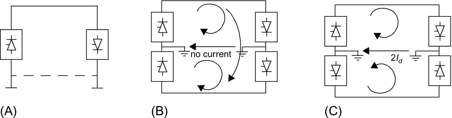
27.1.4.2 Bipolar Link
A bipolar link (Fig. 27.3B) has two conductors, one positive and the other with negative polarity. Each terminal has two sets of converters of equal rating, in series on the DC side. The junction between the two sets of converters is grounded at one or both ends by the use of a short electrode line. Since both poles operate with equal currents under normal operation, there is zero-ground current flowing under these conditions. Monopolar operation can also be used in the early stages of the development of a bipolar link. Alternatively, under faulty converter conditions, one DC line may be temporarily used as a metallic return with the use of suitable switching.
27.1.4.3 Homopolar Link
In this type of link (Fig. 27.3C), two conductors having the same polarity (usually negative) can be operated with ground or metallic return.
Due to the undesirability of operating a DC link with ground return, bipolar links are mostly used. A homopolar link has the advantage of reduced insulation costs, but the disadvantages of earth return outweigh the advantages.
27.2 Main Components of HVDC Converter Station
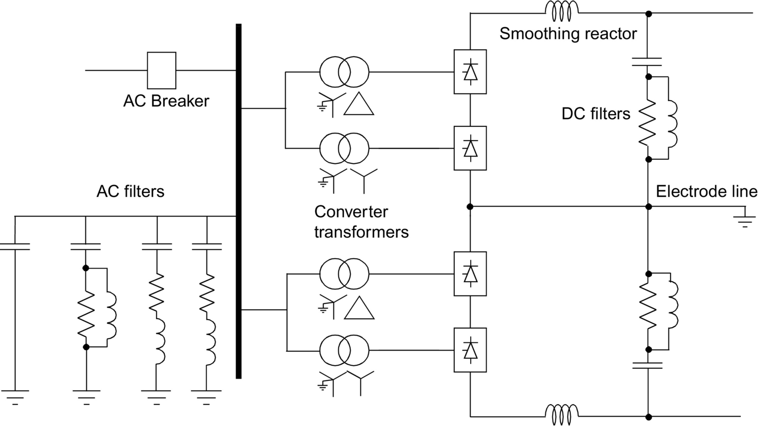
The major components of an HVDC transmission system are the converter stations at the ends of the transmission system. In a typical two-terminal transmission system, both a rectifier and an inverter are required. The role of the two stations can be reversed as controls are usually available for both functions at the terminals. The major components of a typical 12-pulse bipolar HVDC converter station (Fig. 27.4) are discussed below.
27.2.1 Converter Unit
This usually consists of two three-phase converter bridges connected in series to form a 12-pulse converter unit. The design of valves is based on a modular concept where each module contains a limited number of series-connected thyristor levels. The valves can be packaged as either a single-valve, double-valve, or quadruple-valve arrangement. The converter is fed by converter transformers connected in star/star and star/delta arrangements to form a 12-pulse pair.
The valves may be cooled by air, oil, water, or Freon. However, the cooling using deionized water is more modern and considered efficient and reliable. The ratings of a valve group are limited more by the permissible short-circuit currents than by the steady-state load requirements.
Valve firing signals are generated in the converter control at ground potential and are transmitted to each thyristor in the valve through a fiber-optic light guide system. The light signal received at the thyristor level is converted to an electric signal using gate drive amplifiers with pulse transformers. Recent trends in the industry indicate that direct optical firing of the valves with LTT thyristors is also feasible.
The valves are protected using snubber circuits, protective firing, and gapless surge arrestors.
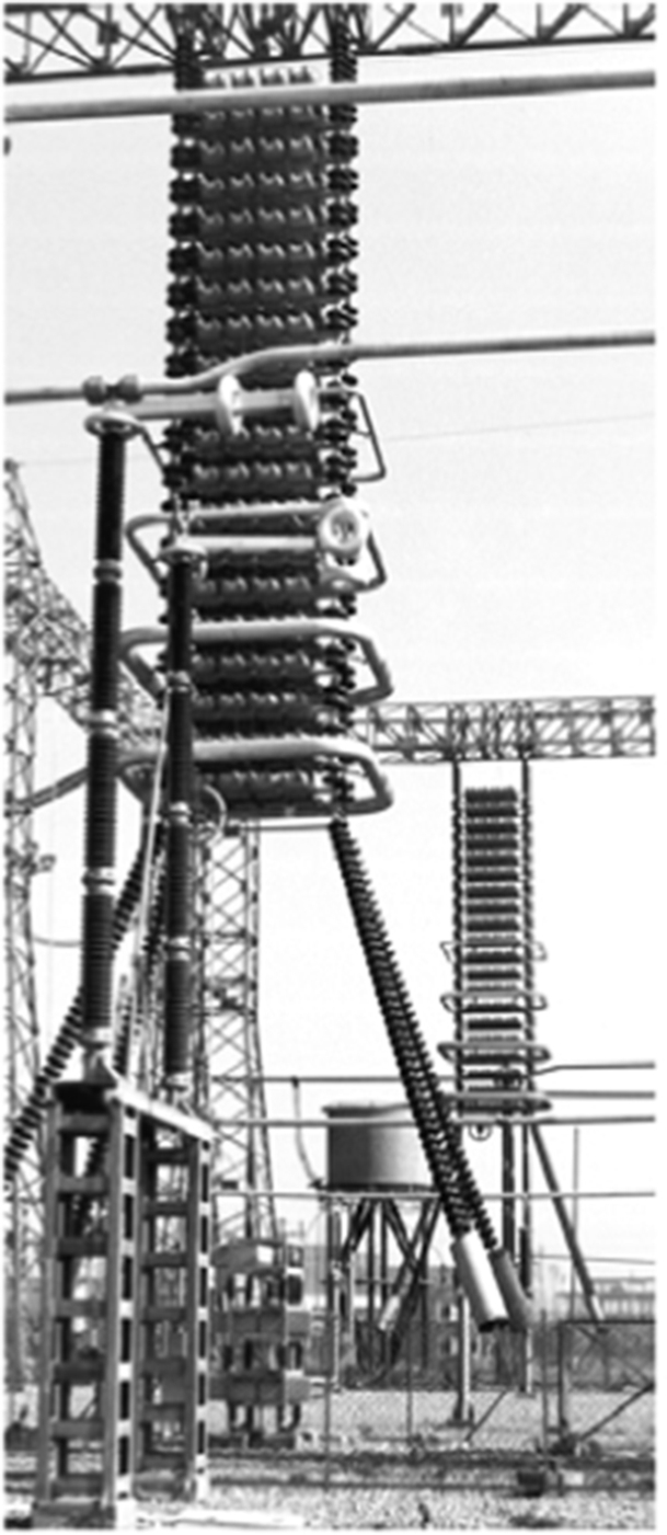
27.2.1.1 Thyristor Valves
Many individual thyristors are connected in series to build up an HVDC valve. To distribute the off-state valve voltage uniformly across each thyristor level and protect the valve from di/dt and dv/dt stresses, special snubber circuits are used across each thyristor level (Fig. 27.5).

The snubber circuit is composed of the following components:
• A saturating reactor is used to protect the valve from di/dt stresses during turn-on. The saturating reactor offers a high inductance at low current and a low inductance at high currents.
• A DC grading resistor RG distributes the direct voltage across the different thyristor levels. It is also used as a voltage divider to measure the thyristor level voltage.
• RC snubber circuits are used to damp out voltage oscillations from power frequency to a few kHz.
• A capacitive grading circuit CFG is used to protect the thyristor level from voltage oscillations at a much higher frequency.
A thyristor is triggered on by a firing pulse sent via a fiber-optic cable from the valve base electronics (VBE) unit at earth potential. The fiber-optic signal is amplified by a gate electronic unit (GEU) that receives its power from the RC snubber circuit during the valve's off period.
The GEU can also effect the protective firing of the thyristor independent of the central control unit. This is achieved by a breakover diode (BOD) via a current-limiting resistor that triggers the thyristor when the forward voltage threatens to exceed the rated voltage for the thyristor. This may arise in a case when some thyristors may block forward voltage, while others may not.
It is normal to include some extra redundant thyristor levels to allow the valve to remain in service after the failure of some thyristors. A metal oxide surge arrestor is also used across each valve for overvoltage protection.
The thyristors produce considerable heat loss, typically 24–40 W/cm2 (or over 1 MW for a typical quadruple valve), and so, an efficient cooling system is essential.
27.2.2 Converter Transformer
The converter transformer (Fig. 27.6) can have different configurations: (i) three phase, two winding; (ii) single phase, three winding; and (iii) single phase, two winding. The valve-side windings are connected in star and delta with neutral point ungrounded. On the AC side, the transformers are connected in parallel with the neutral grounded. The leakage impedance of the transformer (typical value between 15% and 18%) is chosen to limit the short-circuit currents through any valve.
The converter transformers are designed to withstand DC voltage stresses and increased eddy current losses due to harmonic currents. One problem that can arise is due to the DC magnetization of the core due to unsymmetrical firing of valves.
27.2.3 Filters
Due to the generation of characteristic and noncharacteristic harmonics by the converter, it is necessary to provide suitable filters on the AC-DC sides of the converter to improve the power quality and meet telephonic and other requirements. Generally, three types of filters are used for this purpose:
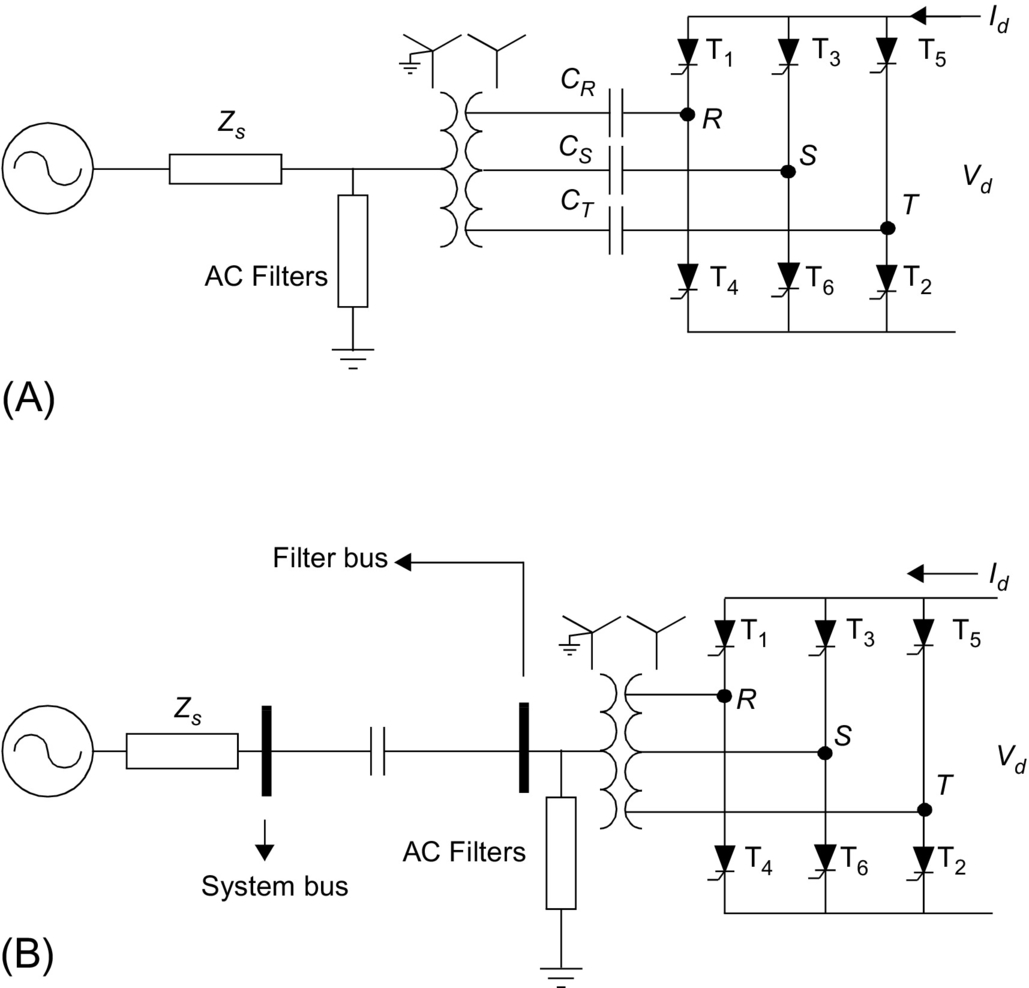
27.2.3.1 AC Filters
AC filters (Fig. 27.7) are passive circuits used to provide low impedance, shunt paths for AC harmonic currents. Both tuned and damped filter arrangements are used. In a typical 12-pulse station, filters at eleventh and thirteenth harmonics are required as tuned filters. Damped filters (normally tuned to the twenty-third harmonic) are required for the higher harmonics. In recent years, C-type filters have also been used since they provide more economic designs. Double- or even triple-tuned filters exist to reduce the cost of the filter (see application example system).
The availability of cost-effective active AC filters will change the scenario in the future.
27.2.3.2 DC Filters
These are similar to AC filters and are used for the filtering of DC harmonics. Usually, a damped filter at the twenty-fourth harmonic is utilized. Modern practice is to use active DC filters (see also the application example system presented later). Active DC filters are increasingly being used for efficiency and space-saving purposes.
27.2.3.3 High Frequency (RF/PLC) Filters
These are connected between the converter transformer and the station AC bus to suppress any high-frequency currents. Sometimes, such filters are provided on the high-voltage DC bus connected between the DC filter and DC line and also on the neutral side.
27.2.4 Reactive Power Source
Converter stations consume reactive power that is dependent on the active power loading (typically about 50%–60% of the active power). Part of this reactive power requirement is provided by the AC filters. In addition, shunt (switched) capacitors and static var systems are also used.
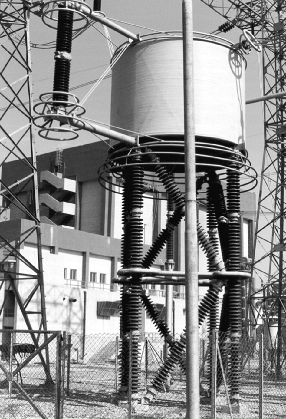
27.2.5 DC Smoothing Reactor
A sufficiently large series reactor is used on the DC side of the converter to smooth the DC current and for the converter protection from line surges. The reactor (Fig. 27.8) is usually designed as a linear reactor and may be connected on the line side, on the neutral side, or at an intermediate location. Typical values of the smoothing reactor are in the 240–600 mH range for long-distance transmission and about 24 mH for a BB connection.
27.2.6 DC Switchgear
This is usually modified AC equipment and used to interrupt only small DC currents (i.e., employed as disconnecting switches). DC breakers or metallic return transfer breakers (MRTB) are used, if required, for the interruption of rated load currents.
In addition to the equipment described above, AC switchgear and associated equipment for protection and measurement are also part of the converter station.
27.2.7 DC Cables
Contrary to the use of AC cables for transmission, DC cables do not have a requirement for continuous charging current. Hence, the length limit of about 50 km does not apply. Moreover, DC voltage gives less aging and hence a longer lifetime for the cable. The new design of HVDC Light cables from ABB is based on extruded polymeric insulating material instead of classic paper-oil insulation that has a tendency to leak. Due to their rugged mechanical design, flexibility, and low weight, polymer cables can be installed underground cheaply with a plowing technique or, in submarine applications, can be laid in very deep waters and on rough sea bottoms. Since DC cables are operated in bipolar mode, one cable with positive polarity and one cable with negative polarity, very limited magnetic fields result from the transmission. HVDC Light cables have successfully achieved operation at a stress of 20 kV/mm.
27.3 Analysis of Converter Bridge
To consider the theoretical analysis of a conventional six-pulse bridge (Fig. 27.9), the following assumptions are made:
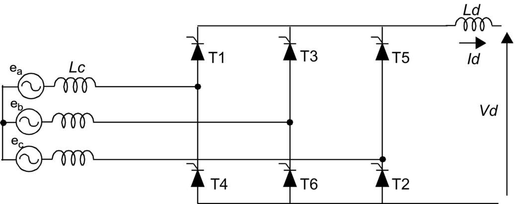
– DC current Id is considered constant.
– Valves are ideal switches.
– AC system is strong (infinite).
Due to the leakage impedance of the converter transformer, commutation from one valve to the next is not instantaneous. An overlap period is necessary, and depending on the leakage, either two, three, or four valves may conduct at any time. In the general case, with a typical value of converter transformer leakage impedance of about 13%–18%, either two or three valves conduct at any one time.
The analysis of the bridge gives the following DC output voltages:
For a rectifier:
where ![]() and
and ![]() .
.
For an inverter:
There are two options possible depending on choice of the delay angle or extinction angle as the control variable:
where
Vdr and Vdi—DC voltage at the rectifier and inverter, respectively
Vdor and Vdoi—open-circuit DC voltage at the rectifier and inverter, respectively
Rcr and Rci—equivalent commutation resistance at the rectifier and inverter, respectively
Lcr and Lci—leakage inductance of converter transformer at rectifier and inverter, respectively
Id—DC current
α—delay angle
β—advance angle at the inverter (β=π−α)
γ—extinction angle at the inverter (γ=π−α−μ)
27.4 Controls and Protection
In a typical two-terminal DC link connecting two AC systems (Fig. 27.10), the primary functions of the DC controls are to
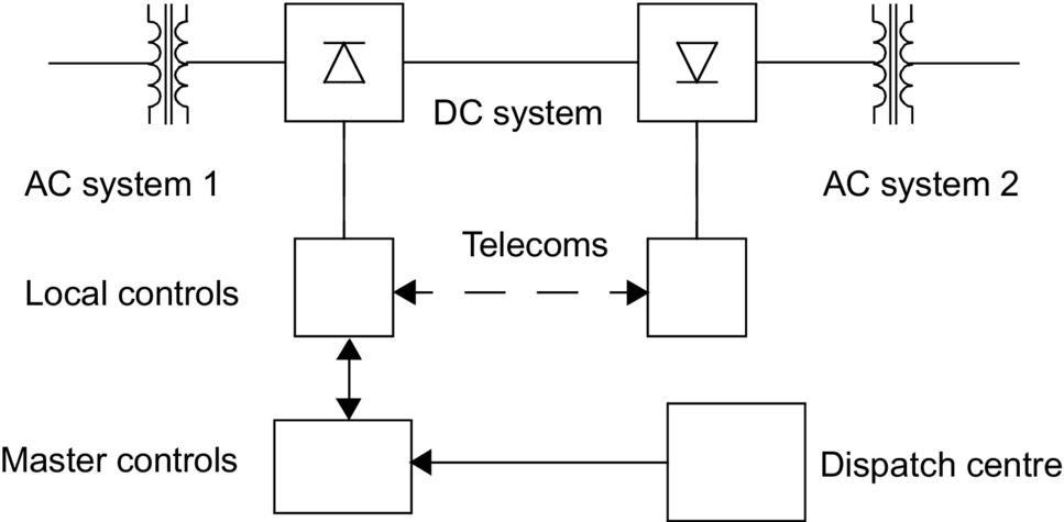
• control power flow between the terminals,
• protect the equipment against the current/voltage stresses caused by faults,
• stabilize the attached AC systems against any operational mode of the DC link.
The DC terminals each have their own local controllers. A centralized dispatch center will communicate a power order to one of the terminals that will act as a master controller and has the responsibility to coordinate the control functions of the DC link. Besides the primary functions, it is desirable that the DC controls have the following features:
• Limit the maximum DC current
Due to a limited thermal inertia of the thyristor valves to sustain overcurrents, the maximum DC current is usually limited to less than 1.2 pu for a limited period of time.
• Maintain a maximum DC voltage for transmission
This reduces the transmission losses and permits optimization of the valve rating and insulation.
• Minimize reactive power consumption
This implies that the converters must operate at a low firing angle. A typical converter will consume reactive power between 50% and 60% of its MW rating. This amount of reactive power supply can cost about 15% of the station cost and comprise about 10% of the power loss.
The desired features of the DC controls are indicated below:
1. Limit maximum DC current—Since the thermal inertia of the converter valves is quite low, it is desirable to limit the DC current to prevent failure in the valves.
2. Maintain maximum DC voltage for transmission purposes to minimize losses in the DC line and converter valves.
3. Keep the AC reactive power demand low at either converter terminal. This implies that the operating angles at the converters must be kept low. Additional benefits of doing this are to reduce the snubber losses in the valves and reduce the generation of harmonics.
4. Prevent commutation failures at the inverter station and hence improve the stability of power transmission.
5. Other features, that is, the control of frequency in an isolated AC system or enhanced power system stability.
In addition to the above desired features, the DC controls will have to cope with the steady-state and dynamic requirements of the DC link, as shown in Table 27.2.
Table 27.2
Requirements of the DC link
| Steady-state requirements | Dynamic requirements |
| Limit the generation of noncharacteristic harmonics | Step changes in DC current or power flow |
| Maintain the accuracy of the controlled variable, that is, DC current and/or constant extinction angle | Start-up and fault-induced transients |
| Cope with the normal variations in the AC system impedances due to topology changes | Reversal of power flow |
| Variation in frequency of attached AC system |
27.4.1 Basics of Control for a Two-Terminal DC Link
From converter theory, the relationship between the DC voltage Vd and DC current Id is given by Eqs. (27.1)–(27.3). These three characteristics represent straight lines on the Vd-Id plane. Notice that Eq. (27.2), that is, beta characteristic, has a positive slope, while the Eq. (27.3), that is, gamma characteristic, has a negative slope. The choice of the control strategy for a typical two-terminal DC link is made according to conditions in Table 27.3.
Table 27.3
Choice of control strategy for two-terminal DC link
| Condition No. | Desirable features | Reason | Control implementation |
| 1 | Limit the maximum DC current, Id | For the protection of valves | Use constant current control at the rectifier |
| 2 | Employ the maximum DC voltage, Vd | For reducing power transmission losses | Use constant voltage control at the inverter |
| 3 | Reduce the incidence of commutation failures | For stability purposes | Use minimum extinction angle control at inverter |
| 4 | Reduce reactive power consumption at the converters | For voltage regulation and economic reasons | Use minimum firing angles |

Condition (27.1) implies the use of the rectifier in constant current control mode. And condition (27.3) implies the use of the inverter in constant extinction angle (CEA) control mode. Other control modes may be used to enhance the power transmission during contingency conditions depending upon applications. This control strategy is illustrated in Fig. 27.11.
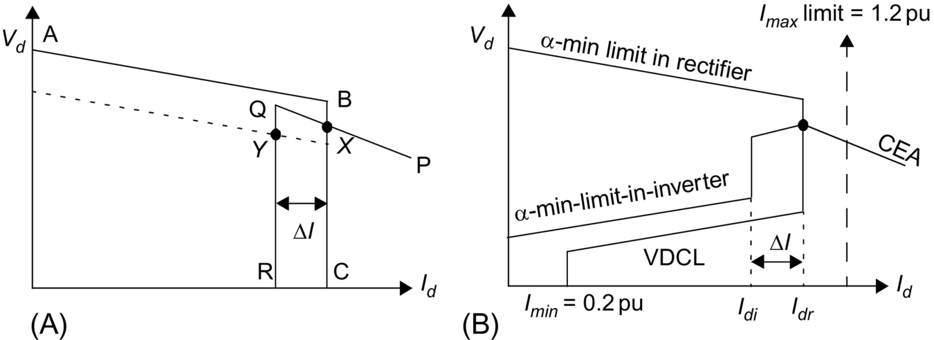
The rectifier characteristic is composed of two control modes: alpha-min (line AB) and constant current (line BC). The alpha-min mode of control at the rectifier is imposed by the natural characteristics of the rectifier AC system and the ability of the valves to operate at alpha equal to zero, that is, in the limit, the rectifier acts as a diode rectifier. However, since a minimum positive voltage is desired before firing of the valves to ensure conduction, an alpha-min limit of about 2–5 degrees is typically imposed.
The inverter characteristic is composed of two modes: gamma-min (line PQ) and constant current (line QR). The operating point for the DC link is defined by the crossover point X of the two characteristics. In addition, a constant current characteristic is also used at the inverter. However, the current demanded by the inverter Idi is usually less than the current demanded by the rectifier Idr by the current margin ΔI that is typically about 0.1 pu; its magnitude is selected to be large enough so that the rectifier and inverter constant current modes do not interact due to any current harmonics that may be superimposed on the DC current. This control strategy is termed the current margin method.
The advantage of this control strategy becomes evident if there is a voltage decrease at the rectifier AC bus. The operating point then moves to point Y. This way, the current transmitted will be reduced to 0.9 pu of its previous value, and voltage control will shift to the rectifier. However, the power transmission will be largely maintained near to 90% of its original value.
The control strategy usually employs the following other modifications to improve the behavior during system disturbances:
At the rectifier:
1. Voltage-dependent current limit, VDCL
This modification is made to limit the DC current as a function of either the DC voltage or, in some cases, the AC voltage. This modification assists the DC link to recover from faults. Variants of this type of VDCL do exist. In one variant, the modification is a simple fixed value instead of a sloped line.
2. Id-min limit
This limitation (typically 0.2–0.3 pu) is to ensure a minimum DC current to avoid the possibility of DC current extinction caused by the valve current dropping below the hold-on current of the thyristors, an eventuality that could arise transiently due to harmonics superimposed on the low value of DC current. The resultant current chopping would cause high overvoltages to appear on the valves. The magnitude of Id-min is affected by the size of the smoothing reactor employed.
At the inverter:
1. Alpha-min limit at inverter
The inverter is usually not permitted to operate inadvertently in the rectifier region, that is, a power reversal occurring due to, say, an inadvertent current margin sign change. To ensure this, an alpha-min limit in inverter mode of about 100–110 degrees is imposed.
2. Current error region
When the inverter operates into a weak AC system, the slope of the CEA control mode characteristic is quite steep and may cause multiple crossover points with the rectifier characteristic. To avoid this possibility, the inverter CEA characteristic is usually modified into either a constant beta characteristic or a constant voltage characteristic within the current error region.
27.4.2 Control Implementation
27.4.2.1 Historical Background
The equidistant pulse firing control systems used in modern HVDC control systems were developed in the mid-1960s [5,6]; although improvements have occurred in their implementation since then, such as the use of microprocessor-based equipment, their fundamental philosophy has not changed much. The control techniques described in Refs. [5,6] are of the pulse frequency control (PFC) type as opposed to the now-out-of-favor pulse phase control (PPC) type. All these controls use an independent voltage-controlled oscillator (VCO) to decouple the direct coupling between the firing pulses and the commutation voltage, Vcom. This decoupling was necessary to eliminate the possibility of harmonic instability detected in the converter operation when the AC system capacity became nearer to the power transmission capacity of the HVDC link, that is, with the use of weak AC systems. Another advantage of the equidistant firing pulse controls was the elimination of noncharacteristic harmonics during steady-state operation. This was a prevalent feature during the use of the earlier individual phase control (IPC) system where the firing pulses were directly coupled to the commutation voltage, Vcom.
27.4.2.2 Firing Angle Control
To control the firing angle of a converter, it is necessary to synchronize the firing pulses emanating from the ring counter to the AC commutation voltage that has a frequency of 60 Hz in steady state. However, it was noted quite early on (the early 1960s) that the commutation voltage (system) frequency is not a constant, neither in frequency nor amplitude, during a perturbed state. However, it is the frequency that is of primary concern for the synchronization of firing pulses. For strong AC systems, the frequency is relatively constant and distortion free to be acceptable for most converter type applications. But as converter connections to weak AC systems became required more often than not, it was necessary to devise a scheme for synchronization purposes that would be decoupled from the commutation voltage frequency for durations when there were perturbations occurring on the AC system. The most obvious method is to utilize an independent oscillator at 60 Hz, which can be synchronously locked to the AC commutation voltage frequency. This oscillator would then provide the (phase) reference for the generation of firing pulses to the ring counter during the perturbation periods and would use the steady-state periods for locking in step with the system frequency. The advantage of this independent oscillator would be to provide an ideal (immunized and clean) sinusoid for synchronizing and timing purposes. There are two possibilities for this independent oscillator:
• Variable frequency operation
Use of a fixed-frequency oscillator (although feasible and called the pulse phase control oscillator) is not recommended, since it is known that the system frequency does drift, between say 55 and 65 Hz, due to the rotating machines used to generate electricity. Therefore, it is preferable to use a variable frequency oscillator (called the pulse frequency control oscillator) with a locking range of between 50 and 70 Hz and the center frequency of 60 Hz. This oscillator would then need to track the variations in the system frequency, and a control loop of some sort would be used for this tracking feature; this control loop would have its own gain and time parameters for steady-state accuracy and dynamic performance requirements.
The control loop for frequency tracking purposes would also need to consider the mode of operation for the DC link. The method widely adopted for DC-link operation is the so-called current margin method.
27.4.3 Control Loops
Control loops are required to track the following variables:
(a) The ordered current Ior at the rectifier and the inverter
(b) The ordered extinction angle (γo) at the inverter
27.4.3.1 Current Control Loops
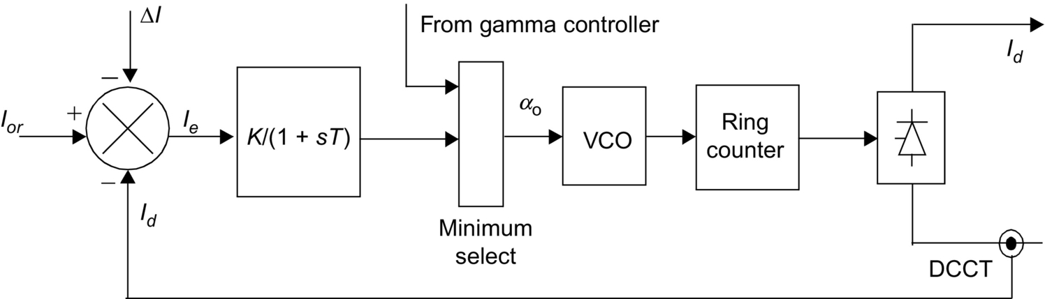
In conventional HVDC systems, a PI regulator is used (Fig. 27.12) for the rectifier current controller. The rectifier plant system is inherently nonlinear and has a relationship given in Eq. (27.1). For constant Id and for small changes in α, we have


It is obvious from Eq. (27.4) that the maximum gain (ΔVd/Δα) occurs when α=90 degrees. Thus, the control loop must be stabilized for this operation point, resulting in slower dynamic properties at normal operation with α within the range 12–18 degrees. Attempts have been made to linearize this gain and have met with some limited success. However, in practical terms, it is not always possible to have the DC link operating with the rectifier at 90 degrees due to harmonic generation and other protection elements coming into operation also. Therefore, optimizing the gains of the PI regulator can be quite arduous and take a long time. For this reason, the controllers are often pretested in a physical simulator environment to obtain approximate settings. Final (often very limited) adjustments are then made on-site.
Other problems with the use of a PI regulator are listed below:
• It is mostly used with fixed gains, although some possibility for gain scheduling exists.
• It is difficult to select optimal gains, and even then, they are optimal over a limited range only.
• Since the plant system is varying continually, the PI controller is not optimal.
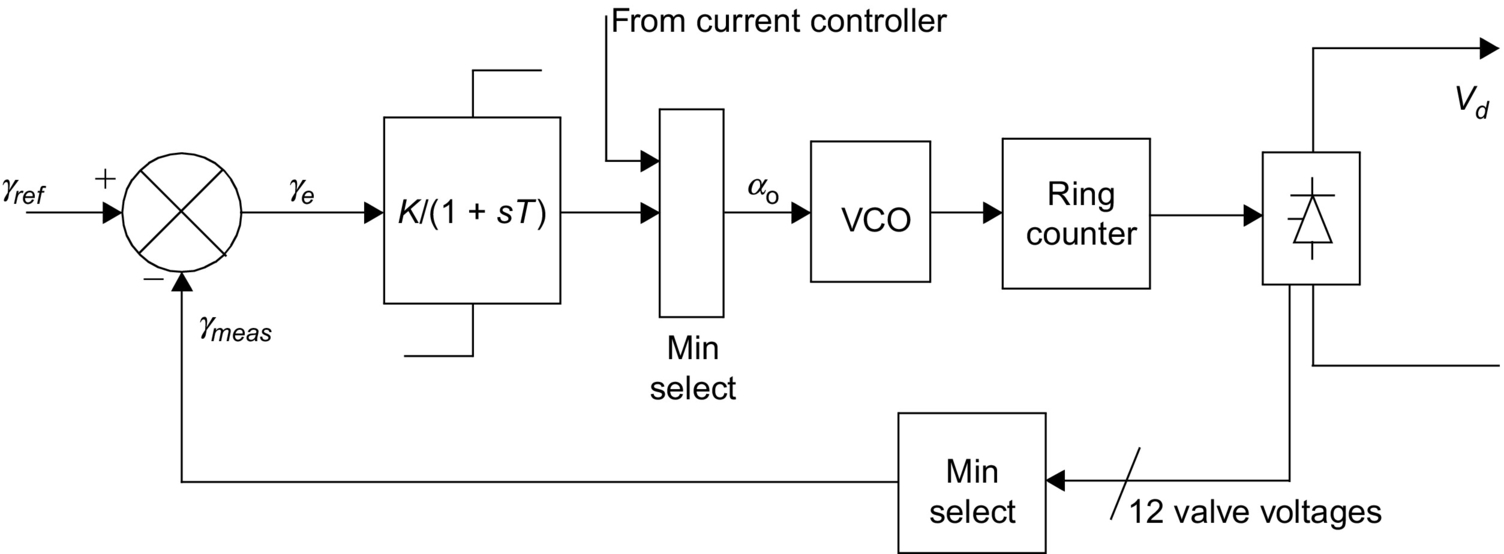
A similar current control loop is used at the inverter (Fig. 27.13). Since the inverter also has a gamma controller, the selection between these two controllers is made via a MINIMUM SELECT block. Moreover, in order to bias the inverter current controller off, a current margin signal ΔI is subtracted from the current reference Ior received from the rectifier via a communication link.
Telecommunication requirements
As was discussed above, the rectifier and inverter current orders must be coordinated to maintain a current margin of about 10% between the two terminals at all times; otherwise, there is a risk of loss of margin, and the DC voltage could run down. Although, it is possible to use slow voice communication between the two terminals and maintain this margin, the advantage of fast control action possible with converters may be lost for protection purposes. For maintaining the margin during dynamic conditions, it is prudent to raise the current order at the rectifier first followed by the inverter; in terms of reducing the current order, it is necessary to reduce at the inverter first and then at the rectifier.
27.4.3.2 Gamma Control Loop
At the inverter end, there are two known methods for the gamma control loop. The two variants are different only due to the method of determining the extinction angle:
– Predictive method for the indication of extinction angle (gamma)
– Direct method for actual measurement of extinction angle (gamma)
In either case, a delay of one cycle occurs from the indication of actual gamma and the reaction of the controller to this measurement. Since the avoidance of a commutation failure often takes precedence at the inverter, it is normal to use the minimum value of gamma measured for the 6 or 12 inverter valves for the converter(s).
1. Predictive method of measuring gamma
The predictive measurement tries to maintain the commutation voltage-time area after commutation larger than a specified minimum value. Since the gamma prediction is only approximative, the method is corrected by a slow feedback loop that calculates the error between the predicted value and actual value of gamma (one cycle later) and feeds it back.
The predictor calculates continuously, by a triangular approximation, the total available voltage-time area that remains after commutation is finished. Since an estimate of the overlap angle μ is necessary, it is derived from a well-known fact in converter theory that the overlap commutation voltage-time area is directly proportional to direct current and leakage impedance (assumed constant and known) value of the converter transformer.
The prediction process is inherently of an individual phase firing character. If no further measures are taken, each valve would fire on the minimum margin condition. To counteract this undesired property, a special firing symmetrizer is used; when one valve has fired on the minimum margin angle, the following two or five valves fire equidistantly. (The choice of either two or five symmetrized valves is mainly a stability question.)
2. Direct method of measuring gamma
In this method, the gamma measurement is derived from a measurement of the actual valve voltage. Waveforms of the gamma measuring circuit are shown in Fig. 27.13. An internal timing waveform, consisting of a ramp function of fixed slope, is generated after being initiated from the instant of anode current zero. This value corresponds to a direct voltage proportional to the last value of gamma. From the gamma values of all (either 6 or 12) valves, the smallest value is selected to produce the indication of measured gamma for use with the feedback regulator (Fig. 27.14).
This value is compared with a gamma-ref value, and a PI regulator defines the dynamic properties for the controller. Inherently, this method has an individual phase control characteristic. One version of this type of control implementation overcomes this problem by using a symmetrizer for generating equidistant firing pulses. The 12-pulse circuit generates 12 gamma measurements; the minimum gamma value is selected and then used to derive the control voltage for the firing pulse generator with symmetrical pulses (Fig. 27.15).

27.4.4 Hierarchy of DC Controls
Since HVDC controls are hierarchical in nature, they can be subdivided into blocks that follow the major modules of a converter station (Fig. 27.16). The main control blocks are as follows:

1. The bipole (master) controller is usually located at one end of the DC link and receives its power order from a centralized system dispatch center. The bipole controller derives a current order for the pole controller using a local measurement of either AC or DC voltage. Other inputs may also be used by the bipole controller such as frequency control for damping or modulation purposes. A communication to the remote terminal of the DC link is also necessary to coordinate the current references to the link.
2. The pole controller then derives an alpha order for the next level. This alpha order is sent to both the positive and negative poles of the bipole.
3. The valve group controllers generate the firing pulses for the converter valves. Controls also receive measurements of DC current, DC voltage, and AC current into the converter transformer. These measurements assist in the rapid alteration of firing angle for protection of the valves during perturbations. A slow loop for control of tap-changer position as a function of alpha is also available at this level.
27.4.5 Monitoring of Signals
As described earlier, monitoring of the following signals is necessary for the controls (Fig. 27.17) to perform their functions and assist in the protection of the converter equipment:

Vd and Id—DC voltage and DC current, respectively,
IAC and I′AC—AC current on line side and converter side of the converter transformer, respectively,
VAC—AC voltage at the AC filter bus.
27.4.6 Protection Against Over-Currents
Faults and disturbances can be caused by malfunctioning equipment or insulation failures due to lightening and pollution. First, these faults need to be detected with the help of monitored signals. Second, the equipment must be protected by control or switching actions. Since DC controls can react within one cycle, control action is used to protect equipment against overcurrent and overvoltage stresses and minimize loss of transmission. In a converter station, the valves are the most critical (and most expensive) equipment that need to be protected rapidly due to their limited thermal inertia.
The basic types of faults that the converter station can experience are the following:
• Current extinction (CE)
CE can occur if the valve current drops below the holding current of the thyristor. This can happen at low-current operation accompanied by a transient leading to current extinction. Due to the phenomena of current chopping of an inductive current, severe overvoltages may result. The size of the smoothing reactor and the rectifier minimum current setting Imin helps to minimize the occurrence of CE.
• Commutation failure (CF) or misfire
In line-commutated converters, the successful commutation of a valve requires that the extinction angle γ-nominal be maintained more than the minimum value of the extinction angle γ-min. Note that γ-nominal=180−α−μ. The overlap angle μ is a function of the commutation voltage and the DC current. Hence, a decrease in commutation voltage or an increase in DC current can cause an increase in μ, resulting in a decrease in γ-nominal. If γ-nominal<γ-min, a CF may result. In this case, the outgoing valve will continue to conduct current, and when the incoming valve is fired in sequence, a short circuit of the bridge will occur.
A missing firing pulse can also lead to a misfire (at a rectifier) or a CF (at an inverter). The effects of a single misfire are similar to those of a single CF. Usually, a single CF is self-clearing, and no special control actions are necessary. However, a multiple CF can lead to the injection of AC voltages into the DC system. Control action may be necessary in this case.
The detection of a CF is based on the differential comparison of DC current and AC currents on the valve side of the converter transformer. During a CF, the two valves in an arm of the bridge are conducting. Therefore, the AC current goes to zero, while the DC current continues to flow.
The protection features employed to counteract the impact of a CF are indicated in Table 27.4.
Table 27.4
Protection against overcurrents
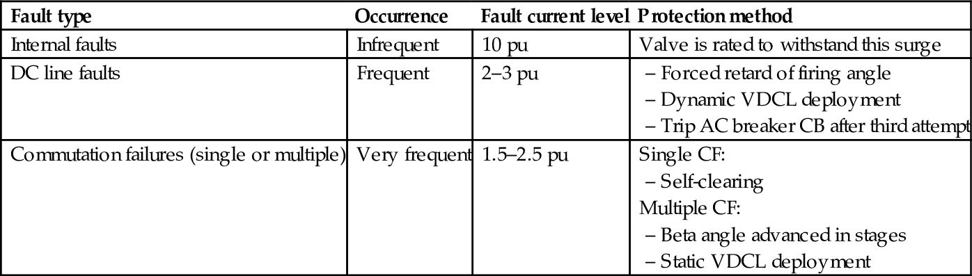
• Short circuits—internal or DC line
An internal bridge fault is rare as the valve hall is completely enclosed and is air-conditioned. However, a bushing can fail, or valve cooling water may leak resulting in a short circuit. The AC breaker may have to be tripped to protect against bridge faults.
The protection features employed to counteract the impact of short circuits are indicated in Table 27.4.
The fast-acting HVDC controls (which operate within one cycle) are used to regulate the DC current for protection of the valves against AC and DC faults.
The basic protection (Fig. 27.18) is provided by the VGP differential protection that compares the rectified current on the valve side of the converter transformer with the DC current measured on the line side of the smoothing reactor. This method is applied because of its selectivity possible due to high impedances in the smoothing reactor and converter transformer.

The OCP is used as a backup protection in case of malfunction in the VGP. The level of overcurrent setting is set higher than the differential protection.
The pole differential protection (PDP) is used to detect ground faults, including faults in the neutral bus.
27.4.7 Protection Against Over-Voltages
The typical arrangement of metal oxide surge arrestors for protecting equipment in a converter pole is shown in Fig. 27.18. In general, overvoltages entering from the AC bus are limited by the AC bus arrestors; similarly, overvoltages entering the converter from the DC line are limited by the DC arrestor. The AC and DC filters have their respective arrestors also. Critical components such as the valves have their own arrestors placed close to these components. The protective firing of a valve is used as a backup protection for overvoltages in the forward direction. Owing to their varied duty, these arrestors are rated accordingly for the location used. For instance, the converter arrestor for the upper bridge is subjected to a higher energy dissipation than for the lower bridge.
Since the evaluation of insulation coordination is quite complex, detailed studies are often required with DC simulators to design an appropriate insulation coordination strategy.
27.5 MTDC Operation
Most HVDC transmission systems are two-terminal systems. A multiterminal DC system (MTDC) has more than two terminals, and there are two existing installations of this type. There are two possible ways of tapping power from an HVDC link, that is, with series or parallel taps.
27.5.1 Series Tap
A monopolar version of a three-terminal series DC link is shown in Fig. 27.19. The system is grounded at only one suitable location. In a series DC system, the DC current is set by one terminal and is common to all terminals; the other terminals are operated at a constant delay angle for a rectifier and constant extinction angle for inverter operation with the help of transformer tap changers.
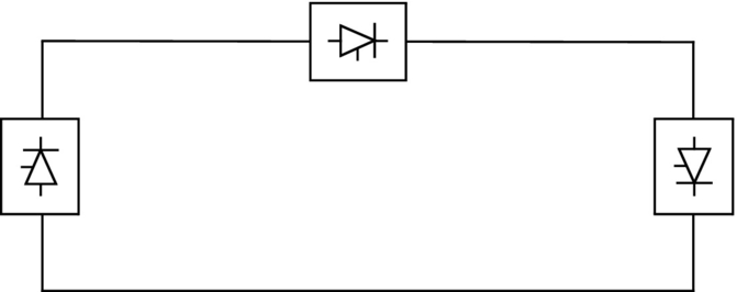
Power reversal at a station is done by reversing the DC voltage with the aid of angle control.
No practical installation of this type exists in the world at present. From an evaluation of ratings and costs for series taps, it is not practical for the series tap to exceed 20% of the rating for a major terminal in the MTDC system.
27.5.2 Parallel Tap
A monopolar version of a three-terminal parallel DC link is shown in Fig. 27.20. In a parallel MTDC system, the system voltage is common to all terminals. There are two variants possible for a parallel MTDC system: radial or mesh. In a radial system, disconnection of one segment of the system will interrupt power from one or more terminals. In a mesh system, the removal of one segment will not interrupt power flow providing the remaining links are capable of carrying the required power.

Power reversal in a parallel system will require mechanical switching of the links as the DC voltage cannot be reversed.
From an evaluation of ratings and costs for parallel taps, it is not practical for the parallel tap to be less than 20% of the rating for a major terminal in the MTDC system.
There are two installations of parallel taps existing in the world. The first is the Sardinia-Corsica-Italy link where a 50 MW parallel tap at Corsica is used. Since the principal terminals are rated at 200 MW, a commutation failure at Corsica can result in very high overcurrents (typically 7 pu); for this reason, large smoothing reactors (2.5 H) are used in this link.
The second installation is the Quebec-New Hampshire 2000 MW link where a parallel tap is used at Nicolet. Since the rating of Nicolet is at 1800 MW, the size of the smoothing reactors was kept to a modest size.
27.5.3 Control of MTDC System
Although several control methods exist for controlling MTDC systems, the most widely utilized method is the so-called current margin method that is an extension of the control method used for two-terminal DC systems.
In this method, the voltage setting terminal (VST) operates at the angle limit (minimum alpha or minimum gamma), while the remaining terminals are controlling their respective currents. The control law that is used sets the current reference at the voltage setting terminal according to
where ΔI is known as the current margin.
The terminal with the lowest voltage ceiling acts as the VST.
An example of the control strategy is shown in Fig. 27.21 for a three-terminal DC system with one rectifier REC and two inverters, INV1 at 40% and INV2 at 60% rating. The REC1 and INV2 terminals are maintained in current control, while INV1 is the VST operating in CEA mode.

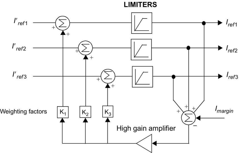
Due to the requirement to maintain current margin for the MTDC system at all times, a centralized current controller, known as the current reference balancer (CRB) (Fig. 27.22), is required. With this technique, reliable two-way telecommunication links is required for current reference coordination purposes. The current orders, Iref1–Iref3, at the terminals must satisfy the control law according to Eqs. (27.5) and (27.6). The weighting factors (K1, K2, and K3) and limits are selected as a function of the relative ratings of the terminals.
27.6 Application
27.6.1 HVDC Interconnection at Gurun (Malaysia)
The 240/600 MW HVDC interconnection between Malaysia and Thailand is a major first step in implementing electric power network interconnections in the ASEAN region. It is jointly undertaken by two utilities, Tenaga Nasional Berhad (TNB) of Malaysia and Electricity Generating Authority of Thailand (EGAT). This will be the first HVDC project for both these utilities. The HVDC interconnection consists of a 110 km HVDC line (85 km owned by TNB and 25 km owned by EGAT) with the DC converter stations at Gurun on the Malaysian side and Khlong Ngae on the Thailand side. The scheme entered into commercial operation in July 2000. The interconnection provides a range of diverse benefits such as
• economic power exchange-commercial transactions,
• emergency assistance to either AC system,
• damping of AC system oscillations,
• reactive power support (voltage control),
• deferment of generation plant up.
27.6.1.1 Power Transmission Capacity
The converter station is presently constructed for monopolar operation for power transfer of 240 MW in both directions with provisions for future extensions to a bipole configuration giving a total power-transfer capability of 600 MW. The HVDC line is constructed with two pole conductors to cater for the second 240 MW pole. Full-length neutral conductors are used instead of ground electrodes because of high land costs and inherently high values of soil resistivity.
The monopole is rated for a continuous power of 240 MW (240 kV and 1000 A) at the DC terminal of the rectifier station. In addition, there is a 10 min overload capability of up to 450 MW, which may be utilized once per day when all redundant cooling equipment is in service.
The HVDC interconnection scheme is capable of continuous operation at a reduced DC voltage of 210 kV (70%) over the whole load range up to the rated DC current of 1000 A with all redundant cooling equipment in service.
27.6.1.2 Performance Requirements
A high degree of energy availability was a major design objective (Fig. 27.23). Guaranteed targets for both stations are the following:

• Forced energy unavailability: <0.43%
• Forced outage rate: <5.4 outages per year
27.6.1.3 Technical Information
See Table 27.6.
27.6.1.4 Major Technical Features
The station incorporates the latest state-of-the-art technology in power electronics and control equipment. The features include the following:
• A fully decentralized control and protection system
• Active DC filter technology
• Hybrid DC current shunt measuring devices
• Triple-tuned AC filter
27.7 Modern Trends
27.7.1 Converter Station Design of the 2000s
The 1500 MW, ±500 kV Rihand-Delhi HVDC transmission system (commissioned in 1991) serves as an example of a typical design of the last decade. Its major design aspects were the following:
• Stations employ water-cooled valves of indoor design with the valves arranged as three quadruple valves suspended from the ceiling of the valve hall.
• Converter transformers are one-phase, three-winding units situated close to the valve hall with their bushings protruding into the valve hall.
• AC filtering is done with conventional, passive, double-tuned, and high-pass units employing internally fused capacitors and air-cored reactors; these filters are mechanically switched for reactive power control.
• DC filtering is done with conventional, passive units employing a split smoothing reactor consisting of both an oil-filled reactor and an air-cored reactor.
• DCCT measurement is based on a zero-flux principle.
• Control and protection hardware is located in a control room in the service building between the two valve halls. The controls still employed some analog parts, particularly for the protection circuits. The controls were duplicated with an automatic switchover to hot standby for reliability reasons.
This design was done in the 1980s to meet the requirements of the day for increased reliability and performance requirements, that is, availability, reduced losses, higher overload capability, etc. However, these requirements led to increased costs for the system.
The next-generation equipment is now being spearheaded by a desire to reduce costs and make HVDC as competitive as AC transmission. This is being facilitated by the major developments of the past decade that have taken place in power electronics. Therefore, the next-generation HVDC equipment will be influenced by the following.
27.7.1.1 Thyristor Development
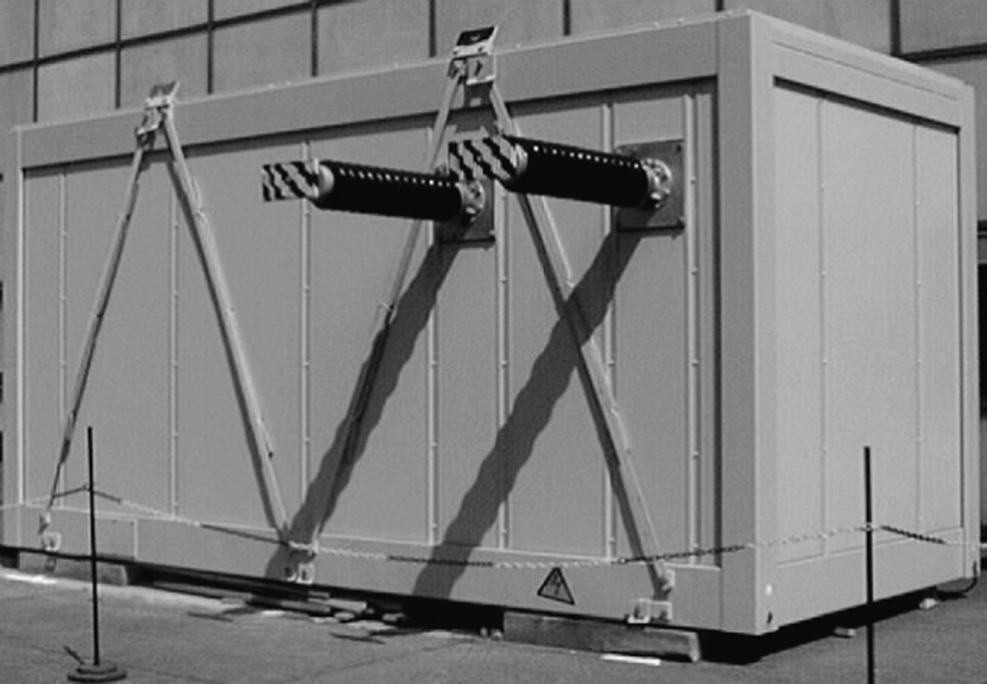
HVDC thyristors are now available with a diameter of 150 mm at a rating of 8–9 kV and power handling capacity of 1500 kW that will lead to a dramatic decrease in the number of series-connected components for a valve with consequential cost reductions and improvement in reliability.
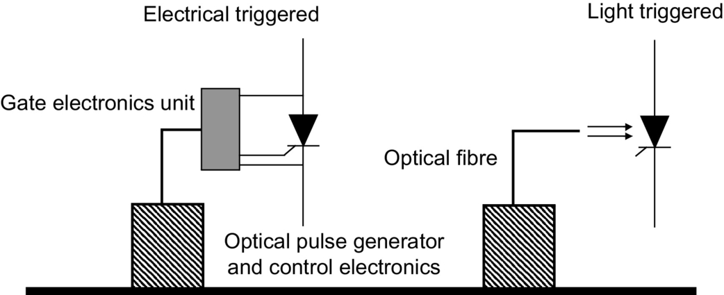
The development of the light-triggered thyristor (LTT) (Figs. 27.24 and 27.25) is likely to eliminate the electronic unit (with their high number of electronic components) for generating the firing pulses for the thyristor (Fig. 27.26). The additional functional requirements of monitoring and protection of the device are being incorporated also.


Both of the above developments present the possibility of achieving compact valves that can be packaged for outdoor construction, thereby reducing the overall cost and reliability of the station.
27.7.1.2 Higher DC Transmission Voltages
For long-distance transmission, there is a tendency to use a high voltage to minimize the losses. The typical transmission voltage has been ±500 kV, although the Itaipu project in Brazil uses 600 kV. The transmission voltage has to balance against the cost of insulation. The industry is considering raising the voltage to ±800 kV.
27.7.1.3 Controls
It is now possible to operate an HVDC scheme into an extremely weak AC system, even with short-circuit capacity down to unity.
Using programmable DSPs has resulted in a compact and modular design that is low cost; furthermore, the number of control cubicles has decreased by a factor of almost 10 times in the past decade. Now, all control functions are implemented on digital platforms. The controls are fully integrated having monitoring, control, and protection features. The design incorporates self-diagnostic and supervisory characteristics. The controls are optically coupled to the control room for reliable operation. Redundancy and duplication of controls is resulting in very high reliability and availability of the equipment.
27.7.1.4 Outdoor Valves
The introduction of air-insulated, outdoor valves will reduce costly requirements for a valve hall. The use of a modular, compact design that will be preassembled in the manufacturing plant will save installation time and provide for a flexible station layout. This design has been feasible because of development of a composite insulator for DC applications that is used as a communication channel for fiber optics, cooling water, and ventilation air between the valve unit and ground.
27.7.1.5 Active DC Filters
This development, made possible due to advances in power electronics and microprocessors, has resulted in a more efficient DC filter operating over a wide spectrum of frequencies and provides a compact design (Fig. 27.27).
27.7.1.6 AC Filters
Conventional AC filters used passive components for tuning out certain harmonic frequencies. Due to the variations in frequency and capacitance, physical aging, and thermal characteristics of these tuned filters, the quality factors for the filters were typically about 100–125, which meant that the filters could not be too sharply tuned for efficient harmonic filtering. The advent of electronically tunable inductors, based on the transductor principle, means that the Q-factors can now approach the natural one of the inductor. This will lead to much more enhanced filtering capacities (Fig. 27.28).

27.7.1.7 AC-DC Current Measurements
The new optical current transducers utilize a precision shunt at high potential. A small optical fiber link between ground and high potential is utilized resulting in a lower probability of a flashover. The optical power link transfers power to high potential for use in the electronic equipment. The optical data link transfers data to ground potential. This transducer results in high reliability, compact design, and efficient measurement (Fig. 27.29).

27.7.1.8 New Topologies
Two new topological changes to the converter design will impact greatly on future designs:
1. Series-compensated commutation:
There are two variants to this topology: the capacitor-commutated converter (CCC) (Fig. 27.30A) and the controlled series capacitor converter (CSCC) (Fig. 27.30B). Essentially, the behavior of the two variants is very similar. The insertion of a capacitor in series with the converter transformer leakage reactance causes a major reduction in the commutation impedance of the converter resulting in a reduction in the reactive power requirement of the converter. An increase in the size of the series capacitor can even result in the converter operation at a leading power factor if so desired. However, the negative impact of a lower commutation impedance results in additional stresses on the valves and transformers and additional cost implications [7].
The first CCC back-to-back converter station (rated at 2×550 MW) has been put into service at Garabi, on the Brazilian side of the Uruguay River. The system interconnects the electric systems of Argentina and Brazil.
2. Voltage-source converters (VSC): The use of self-commutation with the new-generation switching devices (i.e., GTOs and IGBTs) has resulted in the topology of a voltage-source converter (VSC) (Fig. 27.31) as opposed to the conventional converter using line-commutated thyristors and current source converter (CSC) topology. The VSC, being self-commutated, can control active/reactive power and, with PWM techniques, control harmonic generation as well. The application of such circuits is presently limited by the switching losses and ratings of available switching devices. The ongoing advances in power electronic devices are expected to have a major impact on the future application of this type of converter in HVDC transmission. New application areas, particularly in distribution systems, are being actively investigated with this topology. Table 27.5 provides a partial list of the HVDC links in operation using this technique.
One major difficulty for the use of the VSC is the threat posed to the valves from a short circuit on the DC line. Unlike the CSC where the valves are inherently protected against short-circuit currents by the presence of the smoothing reactor, the VSC is relatively unprotected. For this reason, the VSC applications are almost always used with DC cables where the risk of a DC line short circuit is greatly reduced (Table 27.7).
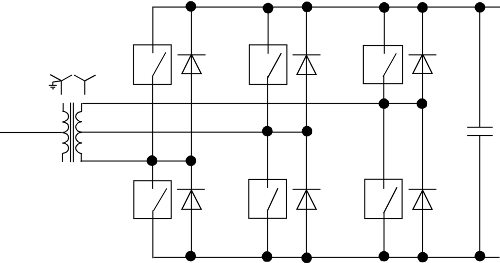
Table 27.5
Main data 1
| Monopolar operation | Rectifier (Malaysia) | Inverter (Thailand) | |
| DC power, Pdn | Rated | 240 MW (stage 1) | 240 MW |
| Max. overload (10 min) | 450 MW | ||
| Minimum (10% of rated) | 24 MW | ||
| DC current, Idn | 1000 A | 1000 A | |
| DC voltage, Udn | 240 kV | 293.5 kV | |
| Firing angle, alpha | 15.0 degrees | – | |
| Extinction angle, gamma | – | 19.6 degrees | |
| Transformer sec. voltage, Uv | 122.2 kV | 122.2 kV | |
| Converter reactive power, QDC | 133.3 MVAr | 150.9 MVAr | |
| Reduced DC voltage operation | 210 kV (70% DC voltage) | ||
| AC system voltage | 275 kV, 50 Hz | 224 kV, 50 Hz | |
| DC transmission line Distance | 110 km |
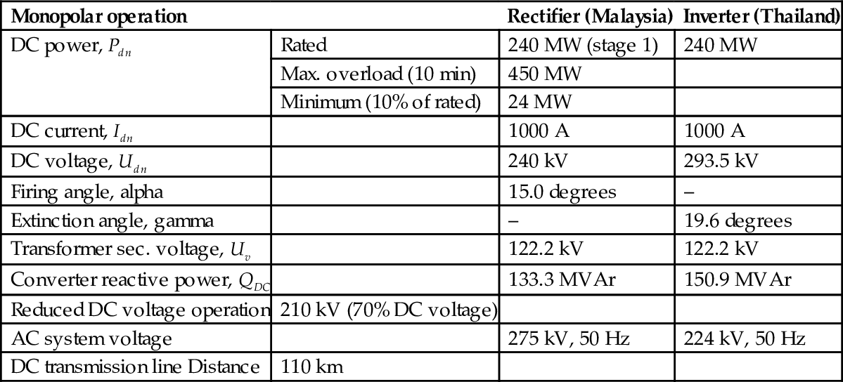
Table 27.6
Main data 2
| Main equipment | GURUN converter station |
| Smoothing reactor | 100 mH |
| DC filter | Active type DC filters including passive type (twelfth/twenty-fourth harmonics) |
| AC filter | 2×60 MVAr (11/13/27) |
| Reactive power compensation | 3×60 MVAr C-shunt |
| Power thyristor Diameter Blocking voltage Max. DC current Max. effective current |
Type T1501 N75T-S34 100 mm 7.5 kV repetitive, 8.0 kV nonrepetitive 1550 A, 120 degrees el., Tc=60°C 3240 A |
| Converter transformer | Single phase, three winding Rated power=275 kV/116 MVA |
| Transmission line Pole conductor Neutral conductor |
Cardinal ACSR 546 mm2, twin conductors per pole Hen ACSR 298 mm2 |
Table 27.7
Applications of HVDC Light technology
| No. | Project | Rating | Distance (km) | Application | Commissioned | |
| MVA | kV | |||||
| 1 | Hellsjon | 3 | ±10 | 10 | AC-DC conversion | Mar. 1997 |
| 2 | Gotland | 50 | ±80 | 70 | Feed from wind power generation | Jun. 1999 |
| 3 | Tjaereborg | 7 | ±10 | 4 | Feed from wind power generation | Aug. 1999 |
| 4 | Directlink | 180 | ±140 | 65 | Asynchronous interconnection | Dec. 1999 |
| 5 | Murraylink | 220 | ±140 | 180 | Asynchronous interconnection | 2002 |
| 6 | Shoreham | 330 | ±140 | 40 | Cross sound cable link | 2002 |
| 7 | Troll A 1&2 | 2×42 | ±60 | 70 | Gas production offshore platform | 2005 |
| 8 | Estlink | 350 | ±150 | 2×74 | Length of land cable, sea crossing, and nonsynchronous AC systems | 2006 |
| 9 | Caprivi Link | 300 | 350 | 950 | Interconnecting grids, energy trade | 2010 |
| 10 | Valhall | 78 | 150 | 292 | Power from shore | 2011 |
| 11 | BorWin1 | 400 | ±150 | 200 | Offshore wind connections | 2012 |
| 12 | East-West Interconnector | 500 | ±200 | 261 | AC voltage control, black start | 2012 |
| 13 | Skagerrak 4 | 700 | 500 | 244 | Interconnecting grids, grid stability | 2014 |
| 14 | Mackinac | 200 | ±71 | DC links in AC grids | 2014 | |
| 15 | DolWin1 | 800 | ±320 | 165 | Offshore wind connection | 2015 |
| 16 | DolWin2 | 900 | ±320 | 135 | Offshore wind connection | 2015 |
| 17 | NordBalt | 700 | ±300 | 450 | Prepare for future DC grid, black start | 2015 |
| 18 | Troll A 3&4 | 2×50 | ±60 | 70 | Power from shore | 2015 |
| 19 | Åland | 100 | ±80 | 158 | Asynchronous networks | 2015 |
| 20 | Maritime Link | 500 | ±250 | 180 | Connecting remote generation | 2017 |
| 21 | Caithness-Moray | 800/1200 | ±350 | 160 | Reinforcement of AC network | 2018 |
| 22 | Johan Sverdrup | 100 | ±80 | 200 | Offshore oilfield | 2019 |
| 23 | Kriegers | Flak | 410 | ±140 | Asynchronous networks | 2019 |
| 24 | NordLink | 2×700 | ±500 | 571 | Interconnecting grids, energy trade | 2020 |
| 25 | NSL | 2(700) | ±515 | 722 | Interconnecting grids, energy trade | 2021 |
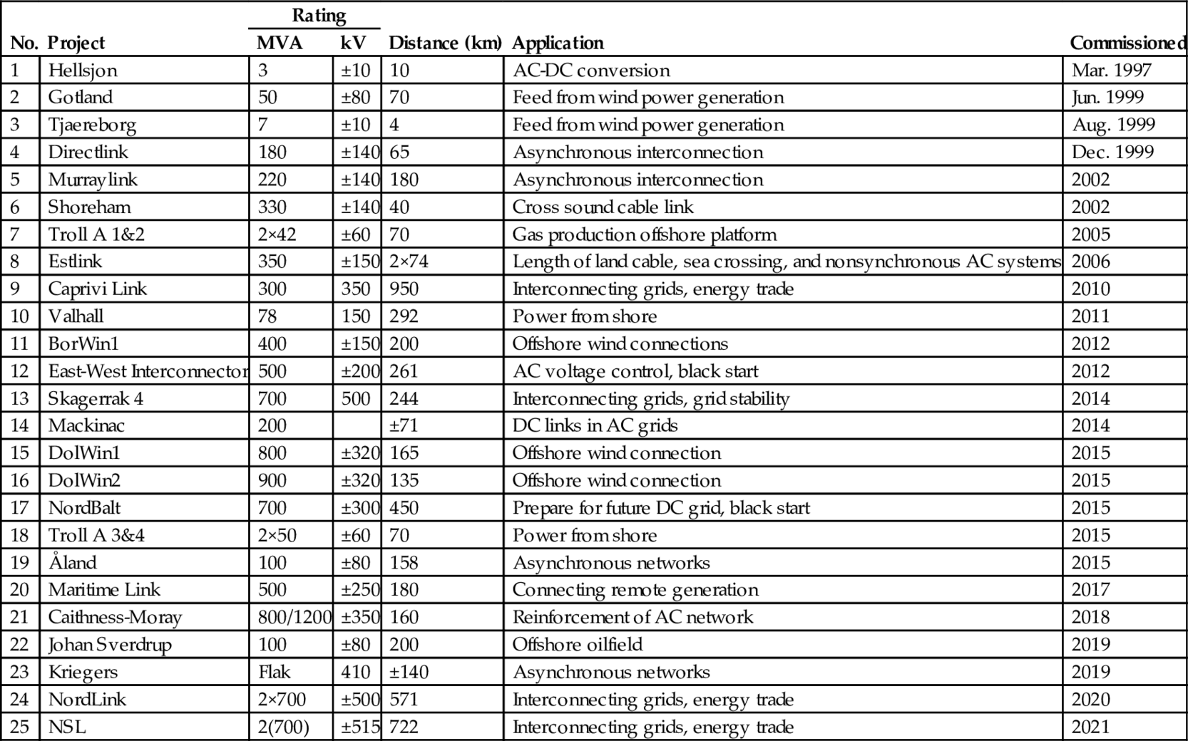
27.7.1.9 Compact Station Layout
The advances discussed above have resulted in marked improvement of the footprint requirement of the compact station [8] of the year 2000 that has about 24% space requirement of the comparable HVDC station designed in the past decade (Fig. 27.32).
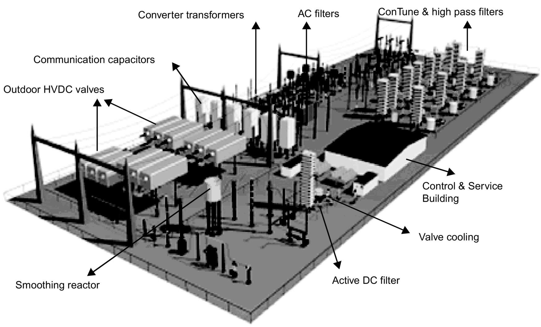
27.8 VSC-HVDC System
27.8.1 Introduction
The existing power transmission networks in most developed countries are heavily loaded that has created the risk of system instability and power quality deterioration. Furthermore, these countries have the problem of obtaining right of ways and face environmental issues for the construction of new transmission lines. The necessity for a new technology by which increased power transmission can be achieved using the existing network infrastructure is clear. As explained earlier, the VSC-HVDC transmission system can take the place of this technology to solve the problem to some extent. The VSC-HVDC system is a relatively mature technology that comprises the high-power, high-frequency semiconductor switches (i.e., IGBTs and GTOs). These devices incorporated with antiparallel diodes make one complete unit. Several units are connected in series to build a valve to get the required voltage level and to increase the redundancy in the converter. The control of these switches is done by using pulse-width modulation (PWM) techniques by which it is possible to control the magnitude and phase angle of the generated fundamental (60 Hz) voltage component. This high controllability of VSC results in a wide range of power system applications like VSC-HVDC, static synchronous compensator (STATCOM), static synchronous series compensator (SSSC), unified power flow controller (UPFC), interline power flow controller (IPFC), and active filters. In addition to bulk power transmission, strategically located VSC-HVDC system in an existing AC power system network augments the network stability and reliability during disturbances and contingencies.
27.8.2 VSC-HVDC System
Fig. 27.33 shows the single-line diagram of a VSC-HVDC system that interconnects two AC networks of same operating frequency for power transmission and stability improvement during contingencies. The system consists of different equipments, such as shunt-connected RLC filters, interfacing transformers, VSCs and their control systems, DC overhead or underground cables, and DC capacitors. The following subsections provide explanations regarding the function of each apparatus comprising the VSC-HVDC.
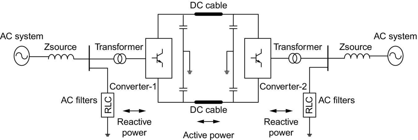
27.8.2.1 AC Shunt RLC-Filters
Switching of high-power, high-frequency switches generates harmonics in the converter output voltages and currents. The order of harmonics generated is directly related to the PWM switching frequency of the semiconductor switches.
Single- or double-tuned low-pass and high-pass damped RLC filters are connected to suppress these harmonics. The frequency modulation index is defined as mf that is defined as the ratio of the switching frequency of the converter to the fundamental frequency of the AC voltage. In the case of three-phase VSC, the harmonics in the line-to-line voltages are present. The odd harmonics exist as sidebands, centered around the mf and its multiples where mf is odd. The value of mf is chosen such that it should be an odd integer to eliminate the even harmonics; also, if it is a multiple of 3, then most of the triplen harmonics are canceled out in the line-to-line voltage.
27.8.2.2 Converter Transformer
A converter transformer interfaces the VSC AC terminals to AC network with suitable voltage level at both sides. It provides electric isolation and operates as a filter between converter and AC networks and provides the appropriate AC voltage level to optimize the available converter valve voltage rating. Configuration and rating of the transformer can be decided from the total system power rating, converter topology, and specified requirements.
27.8.2.3 Voltage Source Converter
The VSC is the main building block of the VSC-HVDC system. The number of switches employed depends on the operating characteristic and voltage level required. The series-connected IGBT switches, connected with antiparallel diodes, make up a valve. Two valves are connected in series to make up the converter leg for one phase. VSC can operate as a rectifier or an inverter at either end depending on the current flow direction. Two converters can be connected as a back-to-back system to connect two different AC grids, DC transmission line, or overhead cables for bulk power transmission or underground cables for connection of offshore oil rigs, islands, or offshore wind farms. The six-switch converter comprises a group of six valves. Different types of PWM techniques are used to operate and control the converter switches. Typical IGBT has rating of 6.5 kV and 2.4 kA. The voltage across the IGBT switch in the ON state is typically in the range of 1–3 V that creates the ON state losses. The switching losses are the second major loss mechanism and are due to fact that, during the turn ON and turn OFF transition, current is still flowing while voltage is present across the device. In order to minimize the switching losses, the maximum switching frequency needs to be carefully considered. VSC is equipped with the RC snubbers and series R-L elements to reduce the dv/dt and di/dt stresses on the switches during ON/OFF transitions.
27.8.2.4 DC Transmission
The DC system can be in the form of a transmission line, with underground or overhead cables. The overhead cables can be used with a moderate size of towers. The extruded polymer cable is a newly developed technique in which the insulation is highly resistant to the DC voltage.
The DC transmission system adopted here is a bipolar transmission system in which the power can flow in both the overhead poles and ground is used as a return path in case of monopolar operation. In case of failure or preplanned maintenance of one pole, reduced power can still be transmitted using the other pole. Two smoothing inductors are connected on DC transmission system to reduce the ripples in the DC current.
27.8.2.5 DC Capacitors
As shown in Fig. 27.33, two series-connected DC capacitors of same size are employed across the DC terminals of converter with grounded midpoint. The size of the capacitor depends on the required DC voltage level and the acceptable DC ripple.
The DC voltage should be adequate for the generation of sinusoidal voltages on AC side of the converter. For the system to operate in the linear range of the PWM, the DC voltage should be 1.634 times the value of root mean square (RMS) AC voltage.
The PWM switching of high-power high-frequency switches generates the harmonics in the DC current flowing in the transmission line. This generates the harmonics in the DC voltage that is strongly related to the converter AC voltage. By evaluation of the magnitude of ripple and the switching frequency of the semiconductor switches, the DC side capacitor ratings can be finalized.
The value of DC capacitor CDC used here can be small, which may result in a faster converter response. The energy stored in the capacitor is released during transients that will help to stabilize the power flow on the DC transmission system. The DC capacitor size is characterized with a time constant τ, which can be defined as the ratio between the energy stored in the capacitor at the rated DC voltage VDC and the apparent power rating of the converter SC:
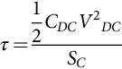
The time constant is equal to the time needed to charge the capacitor from zero to rated voltage VDC if the converter is supplied with a constant active power equal to SC. The time constant τ can be selected to be small to satisfy ripple and transient overvoltage requirement on the DC voltage. A relatively small time constant allows fast control of active power and reactive power.
27.8.3 Topologies of the VSC
VSC can be divided into topologies according to the number of levels for converter output AC voltage, either two level or multilevel. These are explained in following subsections.
27.8.3.1 Two-Level Voltage Source Converter
A two-level bridge is the simplest circuit configuration that can be used to construct a three-phase VSC. It has been widely used in many applications for a range of power levels. As shown in Fig. 27.34, the converter can generate DC voltage waveform of only two values, ±VDC/2, where VDC is the total DC voltage. Relatively simple power and control circuitry, small DC capacitor size, small footprint environmentally, and same semiconductor duty ratio are some of the advantages related to a two-level VSC.

27.8.3.2 Multi-level Voltage Source Converter VSC
Converter topologies with more than two-level voltages are known as multilevel converters. In this type of VSC, the output AC voltage waveform has different level according to the construction of the VSC. The main requirement for multilevel converters is to synthesize a sinusoidal voltage from several voltage levels that are obtained from the DC side capacitor voltages. Multilevel VSCs are divided into different types according to their application. The multilevel VSC found various applications in power systems due to its high power density, excellent performance, and high reliability. Various multilevel topologies are explained next.
27.8.3.3 Neutral Point Diode Clamped VSC
Neutral-point diode-clamped VSC topology is shown in Fig. 27.35. As shown, this topology uses clamping diodes to limit the dynamic and static overvoltages of switching devices. The clamping diodes are connected to the center point of the DC bus capacitor.

The advantages of this topology include reasonable small size of the DC capacitors, small footprint environmentally, and good quality AC output waveform. An n-level diode-clamp converter typically consists of (n-1) capacitors on the DC bus and produces n-levels of the converter output AC voltage. With a higher number of levels, harmonics generation is very low that can even avoid the need for filters in some cases. The disadvantages are related to voltage balancing across the DC capacitors, uneven loss distribution between devices, and excessive clamping diodes necessity in higher levels.
27.8.3.4 Flying Capacitor VSC
Fig. 27.36 shows the three-level flying-capacitor-type VSC topology. This topology uses capacitors instead of diodes in the diode-clamped topology. For an n-level converter, (n−1) numbers of DC capacitors at DC bus and (n−1)×(n−2)/2 number of auxiliary capacitors per phase leg are required. These capacitors are known as floating capacitors.
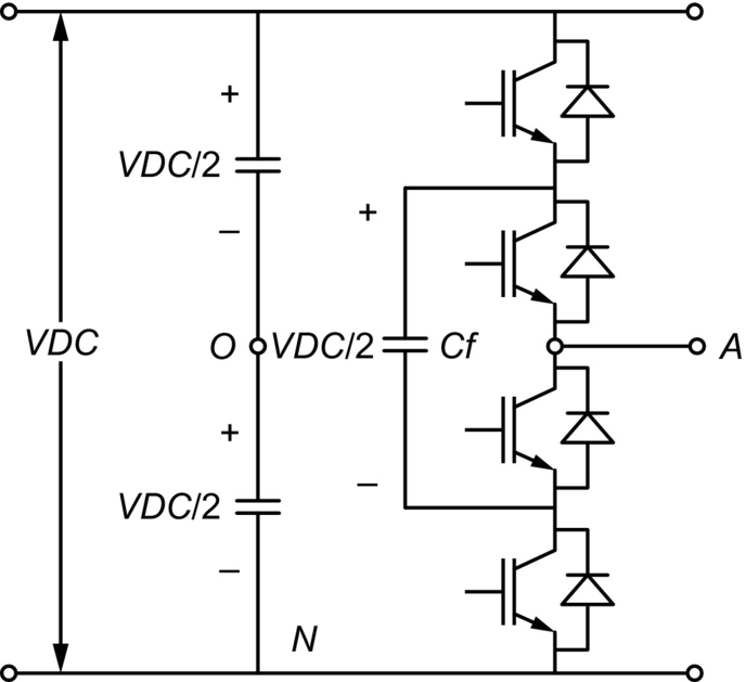
The AC waveform synthesized by this topology is better than the diode-clamped topology. The advantages of this topology are the extra ride through capabilities during power outage and severe disturbances due to large number of storage capacitors, switch combination redundancy for balancing different voltage levels, and avoidance of harmonic filters in higher-level applications. The requirement of an excessive number of storage capacitors on DC side and across the semiconductor switches in higher number of levels makes this topology very expensive. The converter control system is complex, and switching losses are higher compared with diode-clamped topology.
27.8.3.5 ANPC (Actively Neutral Point Clamped) converter
Fig. 27.37 shows the three-level ANPC converter topology in which the clamping diodes are replaced by semiconductor switches. The disadvantage of uneven loss distribution across various devices in the neutral-point diode-clamped converter topology is mitigated by this newly developed topology.

27.8.3.6 Cascaded H-Bridge Converter
This VSC topology (Fig. 27.38) is a cascaded structure that consists of full-bridge inverter units connected in series.

Each unit is fed by a separate DC capacitor, and no other circuit to balance the voltage matching of the switching devices is necessary. There is no need to add the clamping diodes or voltage-balancing capacitors in this topology that results in a relatively simple construction. Main drawback of this topology is the requirement of several independent DC power supplies.
27.8.3.7 Multi-pulse Topologies
In a six-switch converter, the commutation of current takes place six times per cycle. In the case of 12-switch converter, two six-switch converters are connected in series to form a 12-switch converter topology. By using the six-switch converter, the additional multiswitch topologies in multiples of six can be created to form the required pulse level. The 24-switch and 48-pulse converters are implemented in some research papers for application as a STATCOM in power system. The main purpose of using these topologies is to reduce the voltage and current harmonics in the system. As the number of switches increases, the harmonic distortion in the system decreases proportionally.
27.8.4 PWM for VSC
PWM is the most accepted switching technique in which the comparison between a fundamental frequency modulating waveform and a fixed carrier frequency triangular waveform generates the firing pulses for VSC. The magnitude and phase angle of the generated fundamental frequency component of the converter output AC voltage can be controlled by varying the magnitude and phase angle of the modulating waveform. In this technique, the converter output AC voltage contains harmonic frequency components in addition to fundamental frequency component located around the multiples of the triangular waveform carrier frequency.
27.8.4.1 Sinusoidal PWM
The PWM technique used for switching of the semiconductor devices of converter decides the frequency and nature of the converter output AC voltage. So to get the sinusoidal waveform as an output, sinusoidal PWM technique is used. The sinusoidal modulating waveform of 60 Hz system frequency is compared with a high-frequency triangular waveform to generate the pulse-width modulated firing pulses for converter. Two different SPWM methods can be implemented to get the required output.
(a) Bi-polar SPWM
In the case of bipolar sinusoidal PWM method, a single fundamental frequency modulating waveform per phase is compared with the high-frequency triangular waveform. The output voltage switches between −VDC/2 and +VDC/2 voltage levels where VDC is the total DC voltage. It is the reason why this type of switching is called a bipolar PWM switching. As shown in Fig. 27.39, during comparison, when the sinusoidal waveform is greater than the triangular waveform, the PWM trigger signal is high, otherwise at lower level.
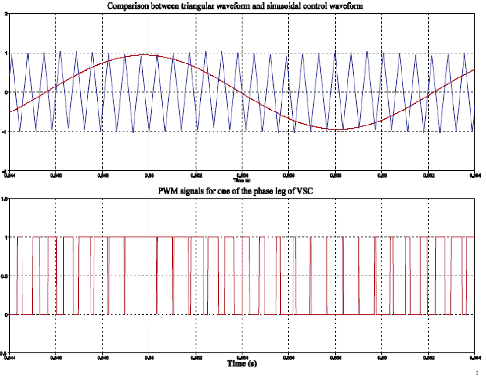
(b) Uni-polar SPWM
In the case of unipolar sinusoidal PWM technique, two same phase fundamental frequency modulating waveforms with opposite polarity are compared with the high-switching-frequency triangular waveforms. The output voltage switches between +VDC/2 and 0 or between 0 and −VDC/2. For this reason, this type of PWM scheme is called a PWM with a unipolar voltage switching.
27.8.5 VSC-HVDC Operation
The VSC-HVDC operation can be explained by considering its operating principle, four-quadrant operation in P-Q diagram, and capability to operate in either rectifier or inverter modes.
27.8.5.1 Operating Principle of VSC-HVDC
The VSC-HVDC operating principle can be explained from the SLD shown in Fig. 27.40, where two AC networks are connected by a VSC-HVDC transmission system.
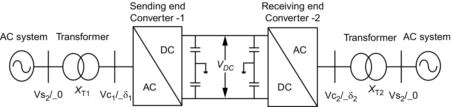
The converter transformer connecting AC network and converter can be modeled as an equivalent series resistance and reactance. The transformer resistance is very small compared with the transformer reactance, so it can be neglected in power calculations. The phase shift between both sides’ voltages due to transformer reactance is responsible for active power flow. At sending end, the voltage VS1 at AC bus is considered as a reference, so the converter output AC voltage VC1 has phase shift δ1 with respect to the bus voltage VS1. The magnitude and phase angle of converter output AC voltage VC1 is controlled by the VSC control system. The active and reactive power flow between the AC system and the converter depends on the magnitude of the voltages at both sides of the transformer, the transformer reactance XT1 and the phase angle δ1 between them. The active and reactive power flow between AC bus and converter AC terminals can be expressed as follows: the active power at sending end and receiving end is given by
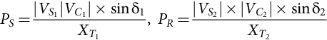
The reactive power at sending end and receiving end is given by

The amplitude, phase angle, and frequency of fundamental component of converter output AC voltage VC1 and VC2 can be controlled using the SPWM technique. If the voltage at the DC side of the converter is VDC that is assumed to be constant, then the fundamental frequency component of converter output AC voltage can be derived from the following equation:
where VDC is the voltage on DC side, ω is the angular frequency, Mi is modulation index, and δ is the phase angle between the converter output AC voltage and the AC bus voltage. Mi can be defined as the ratio of peak value of voltage of modulating waveform (fundamental frequency sinusoidal waveform) to the peak value of voltage of carrier waveform (switching-frequency triangular waveform). From Eq. (27.9), it is seen that the fundamental component of converter voltage depends on the variables Mi, angle δ, and frequency that are independently controlled by VSC controllers. The active and reactive power can be controlled by controlling the phase angle δ and the amplitude of the fundamental frequency component of converter AC output voltage VC, respectively.
In a VSC-HVDC, the polarity of DC voltage is constant, so the power reversal is done by current reversal in the DC link. The current in DC link flows from higher to lower DC voltage level. For stable VSC operation and flow of active power, the DC-link voltage is maintained at a desired reference value by using a feedback control loop. The power flow to and from the AC source can be controlled according to the DC-link voltage requirements. The voltage VDC is measured and controlled in such manner that the DC current flow can be in either direction depending on the requirement of active power flow direction.
27.8.5.2 Four Quadrant Operation of VSC
Active power flow direction for rectifier or inverter operation and reactive power flow direction for inductive or capacitive operating mode of VSC can be explained by a P-Q circle diagram shown in Fig. 27.41. The diagram explains the ability of VSC to operate in all four quadrants of P-Q circle and to achieve the independent control of active and reactive power. The direction of current flow and hence active power flow decides the rectifier or inverter operation of converter.
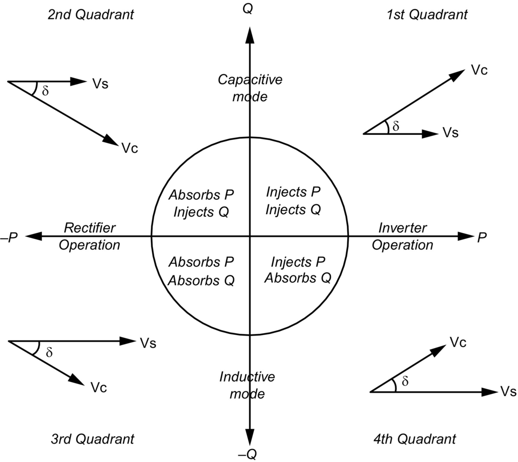
In the first quadrant, both the active and reactive powers are positive, which means that the converter injects both powers to AC system that shows the capacitive mode of inverter operation. The converter output AC voltage magnitude is higher than AC bus voltage and leads AC bus voltage by an angle δ.
In the second quadrant, the active power is negative, and the reactive power is positive, which explains the capacitive mode of rectifier operation. In this case, the converter output AC voltage amplitude is higher than AC bus voltage, but it lags the AC bus voltage by an angle δ.
Both the powers in the third quadrant are negative that means the converter absorbs both powers from the AC system, which explains the inductive mode of rectifier operation. In this case, the AC bus voltage magnitude is higher than the converter output AC voltage, and it leads by an angle δ.
In the fourth quadrant, the active power is positive, and the reactive power is negative, which explains the inductive mode of inverter operation. Here, the converter output AC voltage leads the AC bus voltage, but its magnitude is less than the AC bus voltage.
According to the converter MVA capacity and system requirements, converter can operate in any mode (i.e., capacitive or inductive) of rectifier or inverter operation.
27.8.5.3 Rectifier-Inverter Operation of VSC
The rectifier or inverter operation of VSC can be explained by considering Fig. 27.42. AC bus voltage VS can be taken as a reference, and VC is the converter AC output voltage with phase shift δ. The converter transformer can be represented by an equivalent resistance RT and reactance XT. Two capacitors of same rating 2CDC are connected in series across the DC terminals of the converter. The direction of current flow decides the operation of VSC as a rectifier or inverter.
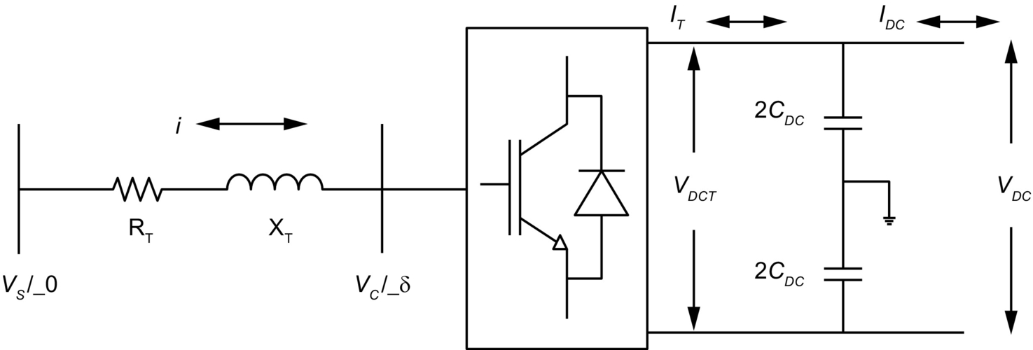
As shown in Fig 27.43, the AC system voltage VS leads the converter AC output voltage VC by an angle δ. The active power flows from the AC system to the converter, so the converter operates as a rectifier. As shown in the figure, ΔV is the voltage drop across the transformer impedance that is controlled in order to control the angle δ. In the rectifier mode of operation, the current IDC is considered positive, and the capacitor CDC is discharged through the DC transmission system. The error signal demands the control circuit for more power from the AC supply. The control circuit thereby generates the appropriate PWM signals for the switching devices, and accordingly, more current flows from the AC to DC side, and the capacitor voltage recovers its predefined value.

As shown in Fig. 27.44, the AC system voltage VS lags the converter AC output voltage by an angle δ. In this case, the active power flows from the converter to AC system, so the converter operates as an inverter. In the inverter mode of operation, IDC becomes negative, and the capacitor CDC is overcharged. The error signal demands the controls to discharge the capacitor CDC and return power to the AC system. The PWM can control both the active power and reactive power independently. Thus, this type of converter can be used for power factor correction also in addition to power transmission.
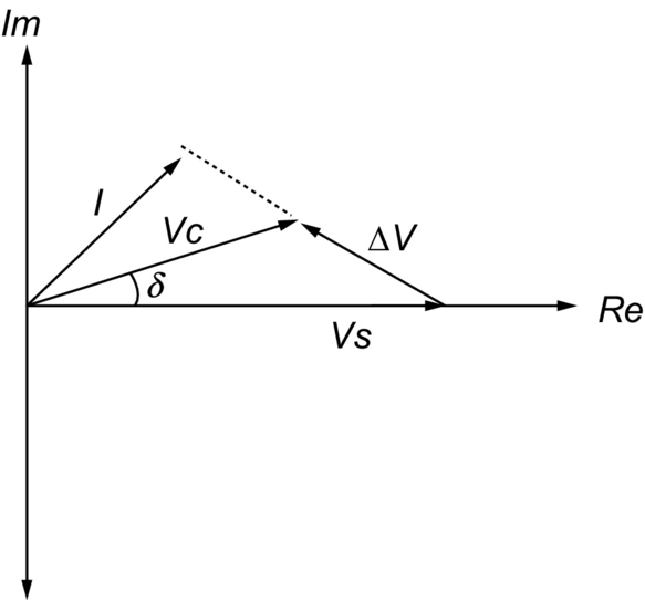
Depending on the control strategy, VSC can be operated as either inverter or rectifier; therefore, it is often referred to as a converter. Two such converters are often cascaded to control the power flow between two AC networks. The first converter converts AC voltage to variable DC-link voltage, and the second converter converts the DC voltage to variable AC voltage with fixed or variable frequency.
27.8.6 Summary
In this chapter, the VSC-HVDC system construction, its principle of operation, and operational function of each component are explained in detail. The different topologies of VSC and PWM techniques are explained. The principle of operation for the VSC-HVDC is explained regarding the active and reactive power flow. P-Q circle diagrams are explained regarding the rectifier/inverter operation and capacitive or inductive mode of operation.
27.9 Control of VSC-HVDC System
27.9.1 Introduction
VSC-HVDC transmission system has flexibility in terms of controlled quantities offering two degrees of freedom at each end to provide stable and robust control. As described in Section 27.8.5, VSC-HVDC system has advantage of independent control of active and reactive power. The direction of active power flow can be changed without changing the DC voltage polarity. The reactive power can be controlled independently at either converter station by controlling converter AC output voltage.
Although both current and voltage control schemes are possible, current control is generally preferred for its excellent dynamic characteristics and inherent overcurrent limitation capabilities. When current control is used, the rectifier input current and inverter output currents are measured and compared with reference signals; the current errors are used as inputs to the PWM modulator, which then provides the required switching signals. The requirements for the control system to operate the VSC-HVDC system are the following:
• It must be capable of controlling the desired active power in either direction.
• The reactive power of system must be controlled independently at both ends.
• The DC voltage must be maintained at desired level for power transfer.
The control modes are chosen according to the application and requirement of the given power system. The rectifier and inverter controllers take the control of any two of abovementioned four control strategies according to the system requirements and operating conditions. VSC1 controllers operate on active power and reactive power control, whereas VSC2 controllers deal with DC voltage and reactive power control (Fig. 27.45).
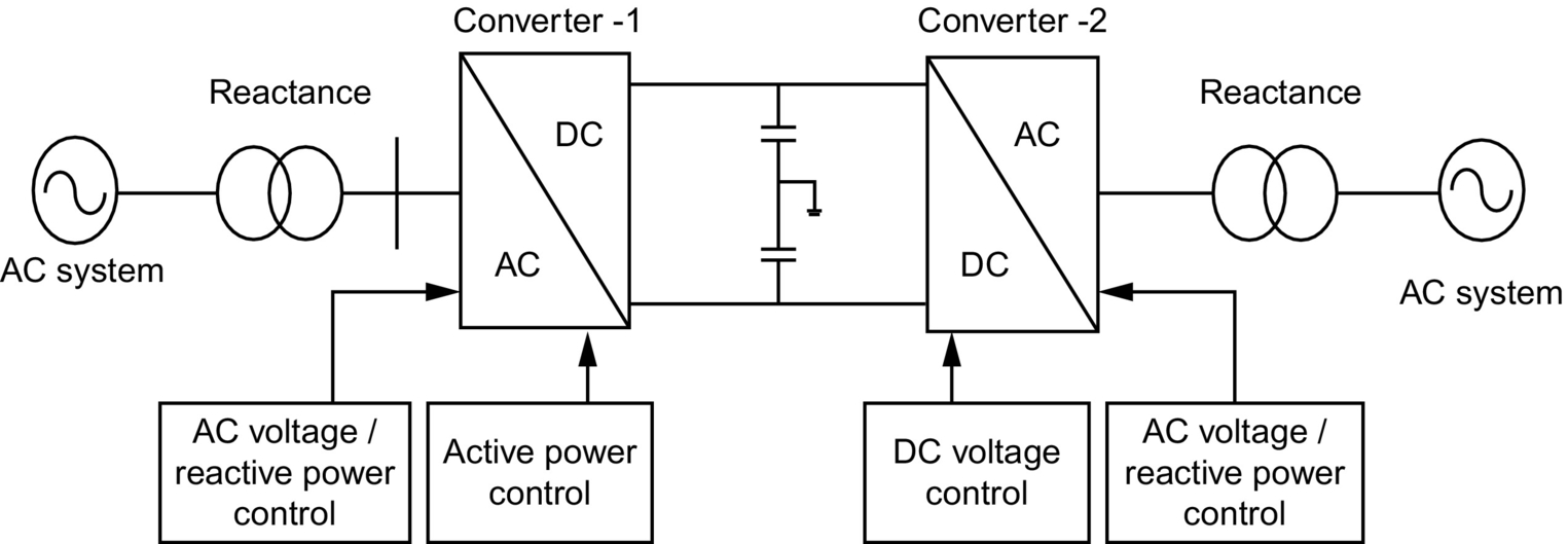
27.9.2 Direct Control Method
Direct control method is a simple method for the control of VSC-HVDC. The angle d and modulation index Mi are controlled directly by using PI controllers. The measured values are compared with the reference values, and the resultant errors are fed to the PI controllers. The output of which is used as either modulation index or angle delta. The modeling of direct control system is provided in Section 27.9.5.3. Though this method is not used in practical applications, it is useful in comparative studies of operation and performance of VSC-HVDC.
27.9.3 Vector Control Method
The P and Q controlled quantities of VSC-HVDC are coupled to each other such that any change in one quantity strongly affects the other. The vector control method removes the coupling between these quantities to ensure the independent control of each quantity. The vector control strategy consists of a cascade control system with faster inner controllers. The vector controller is accomplished by additional outer current controller that provides the reference values for inner controller. The outer controllers include active power controller, reactive power controller, AC voltage controller, DC voltage controller, or frequency controller where the implementation of particular control strategy depends on the application and operating conditions of VSC-HVDC system. It is not possible to implement all the control strategies at the same time and requires an extensive system operation and performance studies for implementation of particular control method.
For feeding the passive system at receiving end without any local voltage source, it is necessary to control the frequency and AC voltage, whereas the active power and reactive power control is required in active AC system. However, since the active power flow into the DC link must be balanced, the DC voltage controller is necessary in any case to achieve active power balance. On the DC side, the active power input to the DC link must equal the active power output from the DC link plus the losses in the DC link. Any difference would result in a change in the DC voltage.
In order to understand the vector control technique of the VSC-HVDC transmission system, the mathematical model for VSC-HVDC system needs to be derived. The vector control strategy can be derived from the mathematical modeling of the system shown in Fig. 27.46.

The AC filters connected to the VSC-HVDC system behave as pure capacitors at fundamental frequencies. Hence, in the mathematical model presented here, the filter resistances and inductances can be neglected. From the single-line diagram (Fig. 27.46), the voltage across the transformer, the current to the filter, and the voltage across the source impedance can be obtained in three-phase instantaneous form as follows:
The voltage across the source impedance is
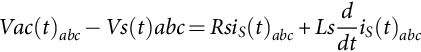
The current through the filters is

The voltage across the transformer is

From Eqs. (27.10)–(27.12), the following differential equations can be derived:

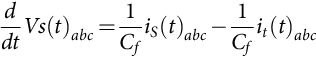
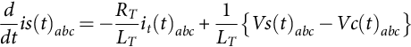
By using Clarke's transformation matrix, quantities from ABC frame can be converted to αβ reference frame as follows:
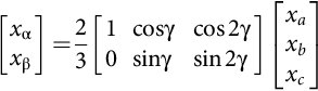
where γ=2π/3.
Eqs. (27.13)–(27.15) can be converted in to αβ frame as follows:
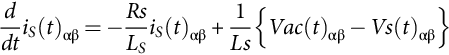
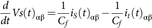

By using the transformation angle θ derived from a phase-locked loop (PLL), the above equations are further transferred to the synchronously rotating dq reference frame, using Park's transformation, as follows:
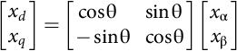


The AC filter voltage, the current through the transformer, and the AC side voltage of VSC can be expressed as

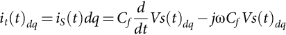

From Eq. (27.26), the dq current component through the transformer can be given as

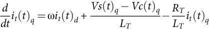
Eqs. (27.27) and (27.28) present the relationship between input reference current and converter output AC voltage in dq reference frame.
27.9.4 Limitations
The VSC-HVDC link with its semiconductor switches has a limited overload capacity. Large transient currents due to system disturbances can stress or damage the converter valves. Therefore, a current limit must be implemented in the control system. Moreover, since the maximum voltage amplitude out of the VSC is limited by the VSC voltage capability, the produced reference voltage from the vector controller must be appropriately limited. The current limit Ilim is compared with the current magnitude computed from the active and reactive reference currents. When the current limit is exceeded, both the active and reactive reference currents have to be limited. The choice of how to limit both reference currents will depend on the application. For instance, if the converter is connected to a strong system, the active component of the reference current will be given priority, when the current limit is exceeded, to produce more active power. The produced active power is estimated from the equation:
If the converter is connected to a weak system or used to supply a bulk industrial user (or island), the VSC will give priority to the reactive component of the reference current to maintain the AC voltage when the current limit is exceeded. The remaining capacity is then available for active power production. The produced reactive and active power may be estimated from the following equations:
where Ilim(q) is the preset maximum reactive reference current.
27.9.5 Outer Controller
The outer controller consists of the DC voltage controller, active power controller and reactive power controller. The proposed simulation model consists of active power and reactive power controllers at VSC1 and DC voltage and reactive power controllers at VSC2. The outer controller creates the reference values of the dq current components for inner current controllers. The outer controller gains are smaller when compared with the inner controller to ensure the stability of the complete system.
27.9.5.1 DC Voltage Controller
As shown in Fig. 27.46, the instantaneous active and reactive powers in dq reference frame at the AC side of the VSC and the power PDC transmitted on the DC side of the VSC are expressed as
where IDCT is the current flowing in the DC terminals of the VSC.
During steady-state operation, the dq components of voltages are constant at the rated values. Therefore, the voltage Vsd is rated voltage Vs, and Vsq is zero. By considering the above assumptions, the active and reactive powers are expressed as follows:
If the losses in the converter transformer and converter are neglected, the power at the AC and DC sides can be considered equal, that is,
Hence,
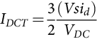
The current in the DC line of the VSC is given as

Any imbalance between the AC and DC powers leads to a change in voltage at the DC-link capacitors, which is given as
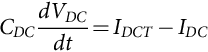
where IDCT is the current in the DC terminals of the VSC, CDC is the total DC side capacitance, VDC is the DC voltage across the capacitor, and IDC is the DC current flowing through the transmission line. The value of DC current from Eq. (27.37) can be used in Eq. (27.35), that is,
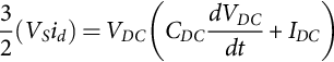
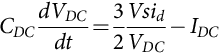
From Eq. (27.39), the value of the reference current id⁎ is derived as follows:

The d-component of the current derived Eq. (27.41) gives the reference current for the inner current controller for DC voltage control.
27.9.5.2 Active Power Controller
The active current reference is obtained from Eq. (27.34):

where Pref is the reference active power. For accurate control of the active power, a combination of a feedback loop and an open loop is used:

where Kp1 and Ki1 are the proportional and integral gains, respectively, of the active power controller.
27.9.5.3 Reactive Power Controller
A reactive power controller similar to the active power controller is obtained from Eq. (27.34) as
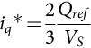
where Qref is reference reactive power. Again, same method is used to combine a feedback loop with an open loop:

where Kp2 and Ki2 are the proportional and integral gains, respectively, of the reactive power controller.
Fig. 27.47 shows active and reactive power control system for VSC1. The control block of PLL is shown from which the synchronization angle θ is derived and fed to the ABC to dq block.

27.9.6 Summary
This chapter deals with the control system of VSC-HVDC transmission system. Two different control systems, direct control and vector control, are explained. The VSC-HVDC mathematical model is provided in this chapter. Block diagram of active power and reactive power control systems in vector control technique is also provided here.
27.10 HVDC System Simulation Techniques
Modern HVDC systems incorporate complex control and protection features. The testing and optimization of these features require powerful tools that are capable of modeling all facets of the system and have the flexibility to do the evaluation in a rapid, effective, and cost-efficient manner.
27.10.1 DC Simulators and TNAs [9]
For decades, this has been achieved with the aid of physical power system simulators or transient network analyzers (TNAs) that incorporate scaled physical models of all power system elements (three-phase DC network lines/cables, sources as emf behind reactances, model circuit breakers for precisely timed AC system disturbances, transformers (system and convertor transformers with capacity to model saturation characteristics), filter capacitors, reactors, resistors, arrestors, and machines). Until the 1970s, these were built with analog components. However, with the developments in microprocessors, it is now feasible to utilize totally digital simulators operating in real time for even the most complex HVDC system studies. Most simulator operating scale are in the range 20–100 V DC and 0.2–1 A AC and at power frequency of 50 or 60 Hz. The stray capacitances and inductances are, however, not normally represented since the simulator is primarily used to assess control system behavior and temporary overvoltages of frequencies below 1000 Hz. Due to the developments of flexible AC transmission system (FACTS) application, most modern simulators now include similarly scaled models of HVDC converters, static compensators, and other thyristor-controlled equipment. The controls of these equipments are usually capable of realistic performance during transients such as the AC faults and commutation failure. The limited availability of adequate models of some of the system elements restricts the scope of the studies that can be completed entirely by means of the simulator. Due to the scaling problems, the losses in the simulator may be disproportionately high and need to be partly compensated by electronic circuits (negative resistances) to simulate appropriate damping of overvoltages and other phenomena.
27.10.2 Digital Computer Analysis
The main type of program employed for studies is an electromagnetic transient program (EMTP) that solves sets of differential equations by step-by-step integration methods. The digital program must allow for modeling of both the linear and nonlinear components (single and three phase) and of the topological changes caused, for example, by valve firing or by circuit-breaker operation. Detailed modeling of the converter control system is necessary depending on the type of study.
EMTP has become an industry standard analysis tool for power systems and is widely used. The program has had a checkered history, and numerous variants have appeared. Initially, the development of the program was supported by the Bonneville Power Administration (BPA). Some of the drawbacks in the capabilities of EMTP became more pronounced as the modeling of flexible AC transmission system (FACTS) with power electronic switches and voltage-source converters became more desirable.
Some of the drawbacks of the original EMTP version were the following:
1. The use of a fixed timestep that did not take into account the relatively long periods of inaction during nonswitching events. This results in unnecessarily long simulation times and huge amounts of data to be manipulated. This is particularly problematic for simulating power electronic converters.
2. The use of a fixed timestep results in the modeled switches chopping inductive currents that causes numerical oscillations. The use of artificial RC “snubbers” helped to alleviate some of these problems. The choice of the snubber capacitor was a function of the magnitude of the current to be chopped and the timestep size.
3. The use of the trapezoidal integration method results in numerical oscillations when the network admittance matrix to be inverted becomes singular. This is the direct result of modeling switches as truly either ON or OFF without representation of their intermediate nonlinear characteristics.
4. The requirement of a one timestep delay between the main program and the TACS subroutine for control simulation.
5. The use of new voltage-source converters with multiple switchings per cycle made the problem of switching “jitter” much more evident.
6. The lack of user-friendly input and output processors.
In recent years, considerable effort has been made by the EMTP Development Coordination Group (DCG) to restructure the program. This has resulted in the latest version called the EMTP restructured version (RV) (see www.emtp.com). The entire code of the program has been rewritten, and graphic input and output processors have been added. A sample of the graphic input file is shown in Fig. 27.48.
The main advantage of digital studies is the possibility of correct representation of the damping present in the system. This feature permits more accurate evaluation of the nature and rate of decay of transient voltages following their peak levels in the initial few cycles and also a more realistic assessment of the peak current and total energy absorption of the surge arrestors. The digital program also allows modeling of stray inductances and capacitances and can be used to cover a wider frequency range of transients than the DC simulator.
The main disadvantage of the digital studies is the lack of adequate representation of commutation failure phenomena with the use of power electronic converters. However, with the increasing capacity of computers, this is likely to be overcome in the future.
The models used in the simulators and digital programs depend on the assumptions made and on the proper understanding of the component and system characteristics; therefore, they require care in their usage to avoid unrealistic results in inexperienced hands.
27.11 Concluding Remarks
HVDC technology is now mature, reliable, and accepted all over the world. From its modest beginning in the 1950s, the technology has advanced considerably and maintained its leading edge image. The encroaching technology of flexible AC transmission systems (FACTS) has learned and gained from the technological enhancements made initially by HVDC systems. FACTS technology may challenge some of the traditional roles for HVDC applications since the deregulation of the electric utility business will open up the market for increased interconnection of networks [7]. HVDC transmission has unique characteristics that will provide it with new opportunities. Although the traditional applications of HVDC transmission will be maintained for bulk power transmission in places like China, India, S. America, and Africa, the increasing desire for the exploitation of renewable resources will provide both a challenge and an opportunity for innovative solutions in the following applications:
• Connection of small dispersed generators to the grid
• Alternatives to local generation
• Feeding to urban city centers