
Design for Reliability of Power Electronic Systems
Yongheng Yang Aalborg University, Aalborg, Denmark
Huai Wang Aalborg University, Aalborg, Denmark
Ariya Sangwongwanich Aalborg University, Aalborg, Denmark
Frede Blaabjerg Aalborg University, Aalborg, Denmark
Abstract
Power density, efficiency, cost, and reliability are the major challenges when designing a power electronic system. Latest advancements in power semiconductor devices (e.g., silicon carbide devices) and topological innovations have vital contributions to power density and efficiency. Nevertheless, dedicated heat sink systems for thermal management are required to dissipate the power losses in power electronic systems; otherwise, the power devices will be heated up and eventually fail to operate. In addition, in many mission critical applications (e.g., marine systems), the operating condition (i.e., mission profiles) is usually harsh, where the input power can change quickly and randomly, resulting in considerable temperature swings in the power electronics. This may induce failures to the power electronic systems. If remain untreated (i.e., ill-designed system without considering reliability), the cost for maintenance will increase, thus affecting the reputation for the manufacturers and, more important, the cost of energy in renewables. Hence, it calls for highly reliable power electronic systems, where the reliability together with various common design parameters should be taken into account in the design phase. Clearly, it is a prerequisite to know the main life-limiting factors in order to predict the lifetime. Then, the design for reliability (DfR) can be performed. In this chapter, the technological challenges in the DfR of power electronic systems are addressed and how the power electronics are loaded considering mission profiles is demonstrated. Further, the DfR approach is systematically exemplified in grid-connected photovoltaic power electronic systems.
Keywords
Reliability; Design for reliability; Power electronics; Failure mechanism; Physics of failure; Mission profile; Thermal loading; Cost of energy; Renewables
45.1 Introduction
Due to the foreseen exhaustion of fossil-based energies, many countries are turning to the renewable energy technologies [1,2]. Among those, wind and solar photovoltaic (PV) systems have attracted more attentions in the past decades [2]. However, the incompatibility of renewable sources and loads requires an intermediate processing stage, which is typically achieved by power electronics [2–4,4a]. In conventional electric systems (e.g., motor drive systems), the role of power electronics is also obvious, as they are heavily involved in controlling the loads—motors. That is, the power electronic technology is the key to optimal energy harvesting and also friendly energy system integration. Moreover, this technology is developing with new and emerging power devices [5,6] with extraordinary performances in terms of switching speed and efficiency. In all, power electronics will be extensively used in many applications in the future.
In practice, the design of power electronic systems is mainly cost-driven, and thus there are three major concerns: power density, efficiency, and reliability [7,8]. Efficiency improvements can be achieved through developing power-lossless topologies (also, including soft-switching techniques) and advancing the power semiconductor devices. As an intuitive way, minimizing the number of conversion stages can contribute to high efficiencies. Notably, the topological simplification also has adverse impacts (e.g., the leakage current issue in transformerless PV inverters), which thus requires new dedicated control strategies. Alternatively, the latest advancements in power semiconductor technologies, for example, wide bandgap power devices like silicon carbide (SiC) transistors, offer much room to improve the efficiency of power electronic systems [6–10]. For instance, as reported in [11–13], the PV power electronic systems with wide bandgap devices have achieved a remarkable efficiency of above 99%, meaning that very few losses exist. The high-efficiency performance has boosted the PV market, where commercial PV inverters employing new devices are available. Furthermore, the wide bandgap power semiconductors feature a high-switching frequency operation capability, and thus, incorporating soft-switching techniques can further improve the efficiency [14].
As discussed above, higher power density and efficiency of power electronic systems are relatively achievable. However, according to a survey [15], the power electronic converter itself has become one of the most fragile parts in the entire system. For instance, in that study, the unscheduled maintenance events due to power electronics account for 37% of the total events in a utility-scale PV power plants, as shown in Fig. 45.1. Those unscheduled maintenance events require human intervention (system repairing or maintenance), thus affecting the overall production and the maintenance costs, as observed in Fig. 45.1. In the end, the cost of PV energy will go up drastically due to the high failure rate of power inverters in PV systems. Hence, as aforementioned, high reliability of power electronics is in urgent need on top of efficiency.

As for reliability, more challenging issues should be addressed [16–23]. Prediction in lifetime of the power electronics is the first task so that the reliability can be taken as a performance factor in the design phase of power electronic systems, which is referred to as the design for reliability (DfR) [24–26]. In the past, the statistical analysis has been the dominant approach for lifetime prediction, where the reliability models (typically, constant failure rates) of subsystems are defined. For instance, a handbook—MIL-HDBK-217 F [27]—has been widely adopted to predict the lifetime of electronic equipment for decades. However, in this handbook, the models are outdated, and the associated failure rates are considered as constants. Thus, this handbook has been revoked. It is also worth to point out that the predicted lifetime or reliability based on this handbook has limited or no direct guiding value for the system design [28]. It is difficult to use the predicted reliability data to design new products or systems with higher reliability, not to mention the control to enhance the reliability performance. With the still increasing demands for high reliability, the analysis approach has to be shifted to the physics-of-failure (PoF) analysis [19–22], where the root causes, failure mechanisms, and mission profiles are in focus [20,29,30]. This (i.e., the PoF-based DfR) enables more predictable and controllable power electronic systems with high reliability.
In light of the above discussion, this chapter briefly discusses the mainstream power electronic converters for wind and PV power systems. More importantly, the DfR approach is explained in detail, including a short description of the failure mechanisms. Case studies on a 6-kW single-phase grid-connected PV inverter system have been provided to better illustrate the DfR approach considering mission profiles. Finally, concluding remarks and discussions on future research trends in the reliability of power electronics are provided.
45.2 Power Electronic Converters and Mission Profiles
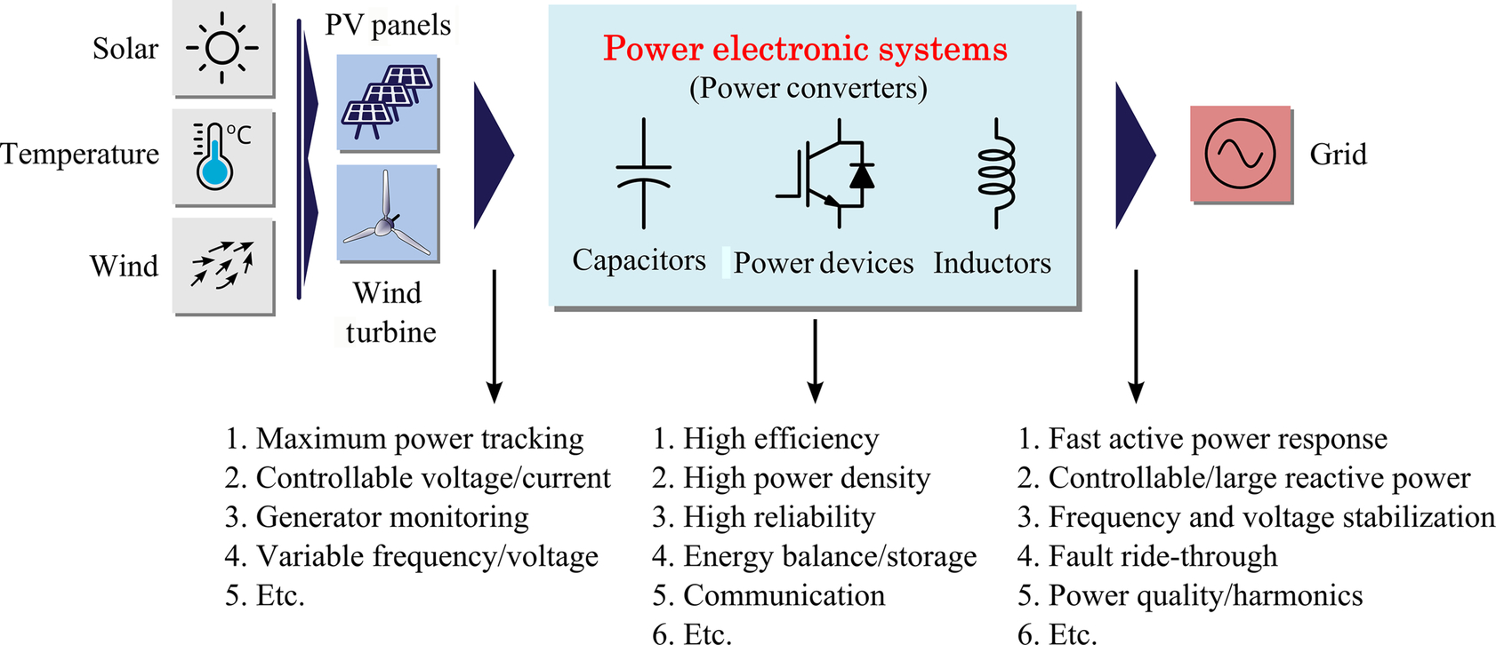
Design and operation of power electronic systems for both wind and PV power systems are strongly dependent on the grid requirements. Fig. 45.2 shows the general demands for grid-connected PV and wind power systems, where the power electronic system is the key component, acting as “the brain” of the entire system. The objectives of those power electronic systems are to manage the power demand from the local operators and end customers [31,32]. A very common requirement is to transfer the PV and wind energy to the grid, according to its inherent characteristics (i.e., applying maximum power point tracking techniques). Other specific demands can be summarized as (a) reliable/secure power supply; (b) high efficiency, low cost, small volume, and effective protection; (c) control of active and reactive power injected into the grid; (d) dynamic grid support (e.g., fault ride-through operation); and (e) system monitoring and communication. In all, as the core of power conversion systems, the reliability of power electronic systems is of strong concern. In the following, some of the state-of-the-art power electronic converter solutions for wind and PV systems are introduced.
45.2.1 Power Electronic Converters for Wind Power Systems
According to the types of generator, power electronics, speed controllability, and the way in which the aerodynamic power is limited, the wind-turbine system (WTS) designs can be categorized into four types:
• Fixed speed wind turbine (WT) systems
• Partial variable speed WT with variable rotor resistance
• Variable speed WT with partial-scale frequency converter
• Variable speed WT with full-scale power converter
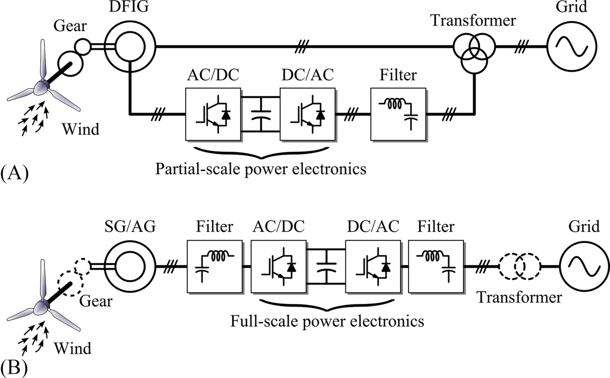
Among those configurations, the latter two shown in Fig. 45.3 currently dominate the markets, which will be further employed in future wind power systems. As observed in Fig. 45.3 and aforementioned, the power electronic converters are very important, and they have various power ratings. In the past, the doubly fed induction generator (DFIG) with partial-scale power electronic converters was the most favorable concept (see Fig. 45.3A). However, the synchronous generator (SG) or asynchronous generator (AG) with full-scale power electronic converters (see Fig. 45.3B) has taken over today's wind power markets [33,34].
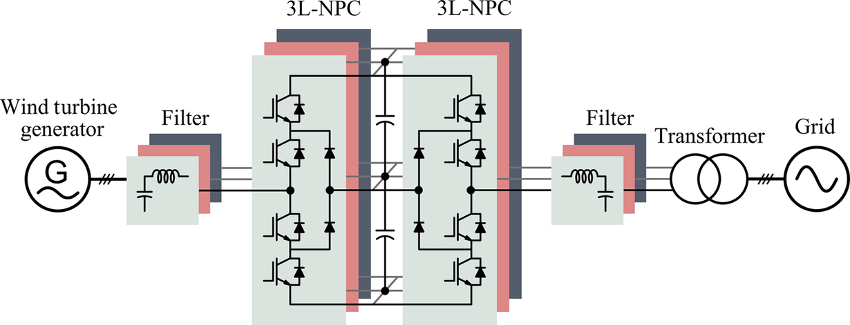
For the power electronic converters, there are many ways to configure. The most commonly adopted three-phase converter is the two-level voltage source converter (2L-VSC), as shown in Fig. 45.4. The popularity of this converter topology lies in its structural and control simplicity. However, the continuous increase in power capacity of an individual wind turbine [35,36] highly stressed the 2L-VSC and thus leading to a lower efficiency. From this standpoint, the multilevel converter technology is getting more and more attentions in wind power applications, since they can achieve more output voltage levels, higher voltage, and larger output power [33–37]. Fig. 45.5 shows the power converter schematics of the most successfully commercialized multilevel converter, that is, the three-level neutral-point-clamped (3L-NPC) converter. As mentioned, the 3L-NPC enables the use of smaller filters (reduced system volume), while the major drawback is the unequal power loss distribution. This in return may challenge the reliability of the entire power electronic converter system. To tackle this issue, multicell converter topologies by connecting converter cells in parallel or in series are developed and also commercially adopted in practice (e.g., Gamesa and Siemens) [38,39].

45.2.2 Power Electronic Converters for PV Power Systems
According to the state-of-the-art technologies, there are certain concepts [26,39a] to organize and deliver the PV power to the grid, as shown in Fig. 45.6. Each of the concepts consists of a couple of power electronic converters (e.g., dc-dc converters and dc-ac inverters) that are configured in different structures, depending on the applications and power ratings. For instance, modular PV converters (Fig. 45.6A) of small volume and high scalability are commonly adopted in small energy conversion systems. However, in order to connect modular PV converters to the grid, high conversion ratio dc-dc converters may be required, or a dc grid is necessary (see Fig. 45.6A and B). In contrast, string, multistring, or central inverters can directly be connected to the grid and they are developed as shown in Fig. 45.6B and C. Nevertheless, when compared with wind power systems, the PV utilization is still at a residential level with lower power ratings. Hence, string and multistring inverters with the exemplified configuration of Fig. 45.6B are dominant on the markets, and the single-phase connection is more often to see [40,41].
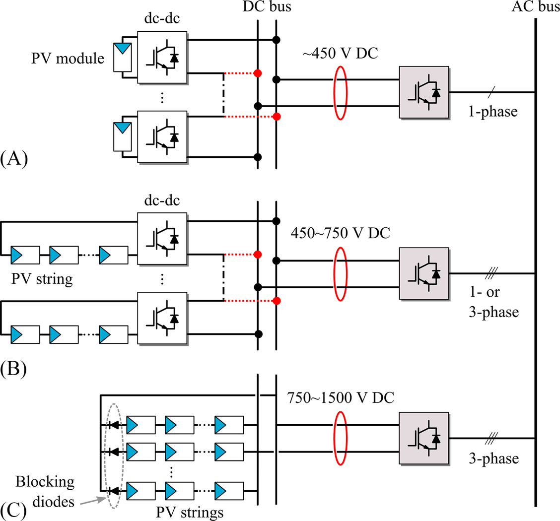
Fig. 45.7 exemplifies a single-phase grid-connected PV system with an LCL filter, where a full-bridge inverter has been employed. Additionally, to have a higher efficiency, transformerless PV inverters are preferred [40]. However, the side effects (e.g., leakage currents) brought by the removal of isolation transformers have to be addressed. Although single-phase configurations are more common, increasing demands in power and voltage also push the ratings of PV systems higher, as demonstrated in Fig. 45.6. Those large PV power plants, rated over tens and even hundreds of megawatts (MW), adopt many central inverters with the power rating of up to 900 kW. A typical large-scale PV power plant is shown in Fig. 45.8, in which the traditional three-phase full-bridge inverter can be adopted. Notably, the cables and power devices may have to bear large currents, and seen from this point, multilevel power electronic converter technologies might be more promising to large-scale PV systems [42–44]. In that case, disconnecting a large amount of dc currents is yet challenging.


45.2.3 Mission Profiles for Power Electronic Converters
A mission profile is normally referred to as a simplified representation of relevant conditions under which the system is operating [45,46]. As a result, the mission profiles for power electronic converters determine the loading of power electronic components, and thereby, they are closely related to the cost and reliability performances. In renewable energy applications, the mission profiles are relatively tough: they need to withstand a large amount of power (even up to a few MWs) and perform a series of complicated functions required from the grid, and meanwhile, they also operate under harsh environments like day-night temperature swings, dust, vibration, humidity, and salty ambience. Moreover, the operating hours for wind turbines can be up to 120,000 h, and for a PV inverter, they might be operating 80,000 h in a 20-year life span [19,20]. Notably, today, even longer operation hours are discussed. In this section, typical mission profiles for wind and PV applications are exemplified, including wind speed, solar irradiance level, and ambient temperature.
45.2.3.1 Wind Speed
As the input of the entire wind power system, the wind energy quantified by the wind speed is an important factor that can determine the design, control, maintenance, energy yield, and eventually also the system cost. During the construction and design phases, assumptions have to be made about the wind conditions that the wind turbines will be exposed to. Typically, wind classes are used that are determined by three parameters—the average wind speed, extreme 50-year gust, and turbulence. Because the loading of power electronic converters are mainly caused by wind speed level and its variations, the knowledge of the wind class is of crucial importance for the reliability calculation and performances. The commonly adopted classifications of wind conditions are from an IEC standard [47]. Fig. 45.9 shows the distribution under different wind classes, where the Weibull function is used to describe the distribution characteristics.

Additionally, a field-recorded annual wind speed profile is illustrated in Fig. 45.10 [48], which is based on 1-h averaged at 80-m hub height for a wind farm located near Germany with the latitude of 54.25° and the longitude of 8.20°. The shown wind speed belongs to the IEC class I—high with an average wind speed of 8.5–10 m/s. It can be seen in Fig. 45.10 that the wind speed fluctuates significantly. Without proper controls of the mechanical and electrical parts, the fluctuations may be transferred to the grid and cause grid stability problems. Moreover, the power electronic components may suffer from largely cyclical loadings and thus accelerating the degradation and challenging the lifetime. As a result, the roughness class and fluctuation of wind speeds should be considered in the control and design of the power electronics for wind power systems [34].

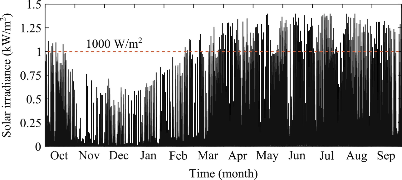
45.2.3.2 Solar Irradiance
Wind speeds directly affect the power outputs of wind power systems, while solar irradiance level and ambient temperature are determining the output power of PV power systems. Actually, the mission profile (i.e., solar irradiance and ambient temperature) is a reflection of the intermittent nature of the solar PV energy, and consequently, it has an inherent relationship with the entire system performance. Figs. 45.11 and 45.12 show annual solar irradiance and ambient temperature profiles for PV systems in Aalborg, Denmark, respectively. It can be observed that both the solar irradiance level and the ambient temperature vary significantly through a year. It is thus required to develop dedicated MPPT control systems in order to increase the energy yield. Moreover, like the case for wind power systems, the resultant fluctuating power from a PV power system may incur stability issues—especially when the PV penetration is getting larger and larger.

45.2.3.3 Ambient Temperature
In many applications, the power electronic systems are exposed to a harsh environment, where the ambient temperature is also time-varying, as shown in Fig. 45.12. The ambient temperature variation inevitably imposes thermal stresses on the power electronic systems, and thus, the reliability is affected by the ambient temperature. For PV power systems, as mentioned previously, the ambient temperature also affects the power outputs. Consequently, those aspects related to mission profiles have to be carefully considered in the control and design phases of power electronic systems.
45.3 Design for Reliability (DfR) of Power Electronic Systems
As discussed in Section 45.2, the power electronic system is the core of the energy conversion or processing system. Hence, the design of the entire system is centered on the power electronic systems, including power density, efficiency, and reliability. All those considered parameters aim to further reduce the cost but increase the manufacturability. For the design of high power density and high efficiency, technological achievements are dictated by topological innovations and semiconductor advancements, as mentioned at the beginning of this chapter.
To design a power electronic system with a specific reliability target, a top-down reliability allocation to the component level is necessary. Fig. 45.13 shows a typical architecture to illustrate this concept. The failure causes of a power electronic system could be hardware, software, and human errors. While this chapter focuses on the hardware reliability, the failure from software and human errors can be considered according to the software reliability modeling and the field operation experiences in human error rates. A certain level of the reliability budget should be allocated for the software failure and human errors accordingly. For the hardware part, there are long-term degradation related wear-out failures and single-event-related catastrophic failures. The wear-out failure of power electronic components usually can be modeled based on long-term operation conditions and their respective lifetime models, which contribute partially to the failure events. The single-event-related catastrophic failure does have associated failure mechanisms, while it is difficult to predict accurately by models. Instead, it can be obtained based on field operation experiences of the products or similar products. An ideal design is to avoid any wear-out failure of power electronic components within the specified service life of the power electronic system of interest. However, it is usually not feasible due to both design cost constraints and component property uncertainties to a certain degree. Based on the budgets for software failures, human errors, single-event-related catastrophic failures, and the system-level reliability target, the reliability design budget of hardware assemblies associated with wear-out failure mechanisms can be determined. The component-level reliability design target can then be allocated. The wear-out failure mechanisms of key power electronic components and the lifetime prediction methods have been well discussed in [20]. As an example, Section 45.4 demonstrates how to size the IGBT power devices to achieve a specific reliability target.
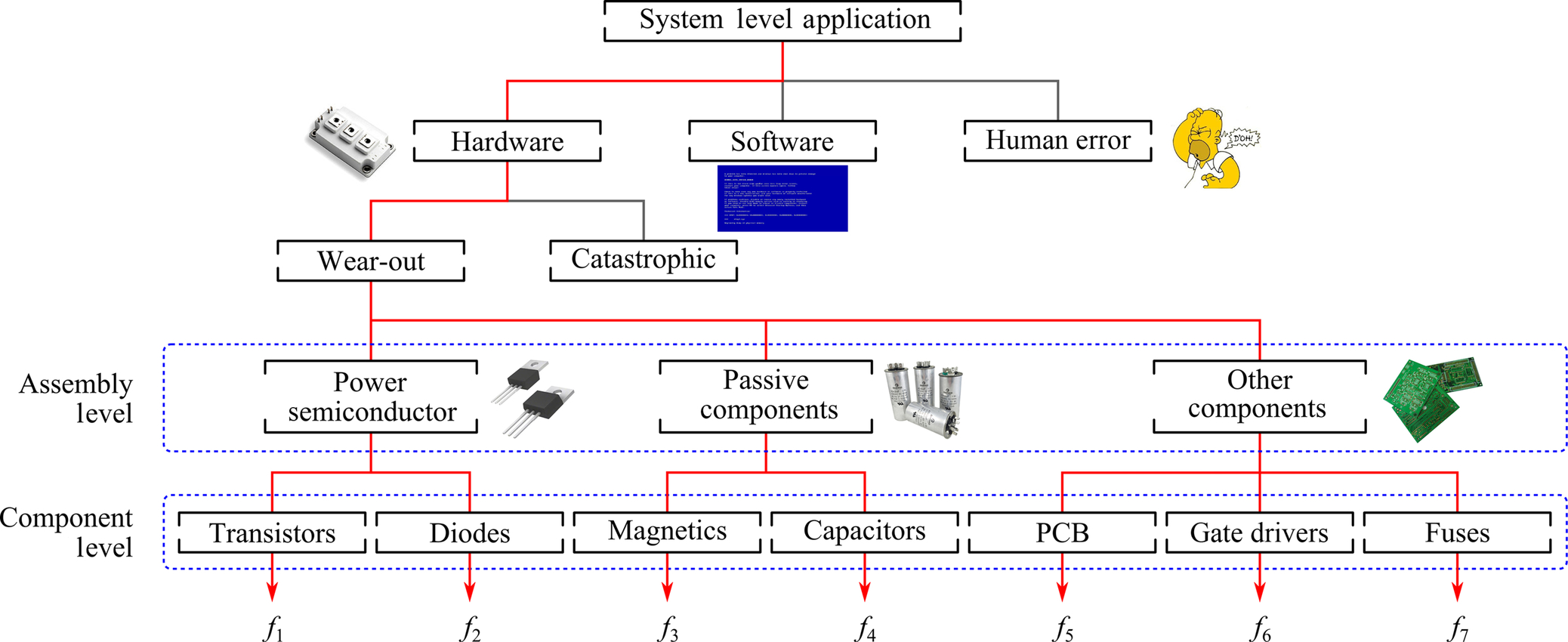
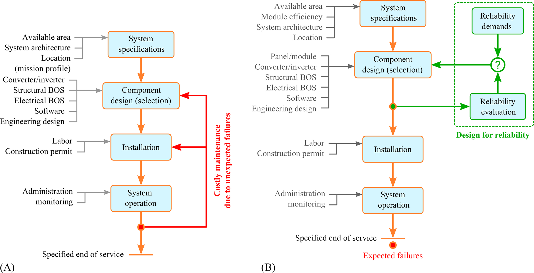
Fig. 45.14A shows the influencing factors in the design and operation phases of power electronic systems, where it can be observed that the design involves many factors. More important, it is seen in Fig. 45.14A that unexpected failures will occur during the operation, resulting in costly maintenance [24]. Accordingly, the design of high reliability is becoming mission critical in power electronic systems, as it is the key parameter affecting the levelized cost of energy (LCOE) [49,50]:
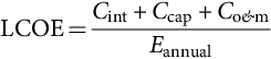
where Cint is the initial development cost, Ccap represents the capital cost, Co&m indicates the operational and maintenance cost, and Eannual denotes the average annual energy production in the lifetime cycle of the system. More specifically, a power electronic system of high reliability will reduce the cost for operational and maintenance and also increase the service time (i.e., more energy production). Eventually, the cost of energy is lowered.
In order to lower the unscheduled maintenance cost, potential failures should be anticipated as early as possible and input into the design flow. This initiates a more promising solution to improving the reliability of power electronic systems, as shown in Fig. 45.14B, being the DfR approach. The inclusion of reliability enables a quick identification of design flaws or weakness and thus feeds back to the design for corrections (e.g., reselection of components). After a few iterations, the reliability demands can be fulfilled before the installation/construction of the power electronic system. As a consequence, significant cost reduction in the design phase and shorter development cycles can be attained while also targeting for higher reliability. Clearly, the failures or downtimes of the designed power electronic systems are predictable, demonstrated in Fig. 45.14B.
It should be pointed out that the reliability prediction is the first task for the DfR process, and it involves in multiple disciplines from the PoF point of view. Fig. 45.15 depicts the detailed reliability evaluation process of the DfR approach, which shows that the reliability analysis has three major tasks:

• Stress analysis and strength modeling
• Reliability mapping.
More specifically, the critical components and the major failure mechanisms of power electronics are identified through physics analysis and real-field experience. Accordingly, the corresponding stresses and the ability of power electronic components to withstand the stresses are tested and modeled. Finally, counting algorithms and statistical distributions are adopted to map the stress and strength information to the reliability metrics of the power electronic system. The reliability indicators can be direct performances like the Bx lifetime, robustness, and failure probability or indirect performances [24]. Here, the Bx lifetime indicates the time by which x percent of a population of the system under study will have failed.
For a specific power electronic system, the DfR approach included in the Fig. 45.14 and the reliability predication process detailed in Fig. 45.15 enable analyzing the power converter candidates in terms of reliability. Here, the failure mechanisms have to be identified first. As discussed in [20], for power electronic converters, the major failures are related to the temperature in power devices. Nevertheless, on condition that the failure mechanisms are identified, it is possible to directly translate mission profiles into thermal loading on the power electronic components of the selected candidates. As a result, the reliability is obtained and can be compared with the demand. The process is further summarized as follows:
• Thermal loading interpretation
• Lifetime model of power devices
• Monte Carlo reliability assessment
• System-level reliability analysis
which is also discussed in detail in the following.
45.3.1 Mission Profile Translation
In the DfR approach, the knowledge of the power converter operating conditions during the entire operation is essential [20,51]. In this respect, a mission profile of the power electronic converters, which represents the operating condition of the system, is needed. Then, the mission profiles have to be translated into thermal loading of power electronic systems (e.g., junction temperature variations of the devices), which can be done in the following way.
Once the mission profiles are obtained, the power production of the power electronic system can be estimated considering the electrical characteristic model. Taking into account the conversion efficiency, the power losses dissipated in the power devices can be estimated. Notably, this loss calculation is usually implemented with a lookup table (LUT), in order to assist the long-term simulation (e.g., an annual mission profile). In that case, the power losses are calculated for a certain set of operating conditions (e.g., the input power from 0 to 100% of the rated power), and the power losses under other operating conditions can be interpolated from the constructed LUT. Then, the thermal model of the power devices in the power electronic converter is required in order to obtain the device junction temperature loading.
45.3.2 Thermal Loading Interpretation
By applying the previous process, the junction temperature of the power electronic device Tj under a specific mission profile can be obtained. However, the device junction temperature is usually an irregular loading profile, due to the dynamics of mission profiles (e.g., the solar irradiance and ambient temperature for PV power systems). Thus, a cycle-counting algorithm such as a rainflow analysis is usually employed, in order to divide the irregular thermal loading cycle into several regular thermal loading cycles [52]. By doing so, the information such as the mean junction temperature Tjm, the cycle amplitude ΔTj, and the cycle period ton can be obtained, which can then be applied to the lifetime (degradation) model of the selected power electronic devices of the converter candidates.
45.3.3 Lifetime Model of Power Devices
Any component in a power electronic system (e.g., power semiconductors and capacitors) can cause failures of the entire system. In that regard, it leads to a complicated analysis, as the components may have a cross effect of the reliability on each other. For simplicity, only the temperature-related failure mechanisms of the power device are considered. In fact, the power device has been reported as one of the most critical components in power electronic systems [15,16]. Hence, it is a natural thought to consider temperature-related lifetime models [53,54].
Normally, the lifetime of the power device is expressed by considering the life consumption (LC), which indicates how much life of the device has been consumed (or damaged) during operations. The LC is calculated by using the Miner's rule as [52]
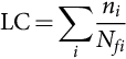
where ni is the number of cycles (obtained from the thermal loading interpretation) for a certain Tjm, ΔTj, and ton, and Nfi is the number of cycles to failure calculated at that specific stress condition. For instance, if the number of cycles ni is counted from an annual mission profile, the LC calculated in (45.2) will represent a yearly LC of the power device. When the LC accumulates to unity, the power electronic device is considered to reach its end of life, and the lifetime for the single power electronic device is predicted.
45.3.4 Monte Carlo Reliability Assessment
Actually, the lifetime prediction of the power device obtained from (45.2) can be taken as an ideal case, where all the power devices fail at the same rate. In reality, there are uncertainties in the time to failure of the power devices, mainly introduced by parametric variations in the lifetime model and changes in the stresses. Therefore, it is more common to express the lifetime prediction in terms of statistical values (e.g., using the probability of failures), rather than the fixed values. In order to do so, a Monte Carlo analysis should be performed, which is aimed to introduce variations in the system parameters, and simulate the result with a large number of samples. With the large enough number of samples, the results will converge to the expected value.
This approach can be employed for estimating the power devices lifetime [55–57]. In this method, all the parameters in the lifetime model have to be modeled by a distribution function with a certain range of variations. Then, following the Monte Carlo simulation approach, a certain number of samples from each parametric distribution are randomly taken to calculate the lifetime of the power electronic device. Accordingly, a set of results is obtained, which can then be represented with a certain distribution function (e.g., Weibull distribution) [58]. The probability density function (PDF) of this lifetime prediction result is usually referred to as a lifetime distribution (failure distribution) f(x), while its cumulative distribution function (CDF) is considered as an unreliability function F(x). Eventually, the Bx lifetime can be obtained from the unreliability function of the power electronic device.
45.3.5 System-Level Reliability Analysis
A power electronic system usually has many power devices, and each power electronic device has its own unreliability function F(x). In order to perform the system-level reliability assessment, the reliability block diagram of the entire system should be constructed [16]. The reliability block diagram represents how the reliability of components in the system interacts with each other. For a system with n components and the entire power electronic system cannot function if any of the n components fails, the total unreliability of system Ftot(x) can be calculated as
where Fn(x) is the unreliability function of the n-th component. Once the total unreliability function of the inverter system Ftot(x) is obtained, the Bx lifetime of the entire power electronic system can be estimated in a similar way as it has been done for a single power electronic component. However, it should be pointed out that the system-level reliability analysis approach (i.e., the reliability block diagram) can be applied to any power electronic system. For different converter topologies, the reliability block diagram may be different from (45.3), depending on the number of power devices and their operational principles.
Following the above steps, the reliability of a power electronic system can be predicted, and then, it can be compared with the design target (i.e., the reliability demand). This DfR flow especially includes the reliability in the design and thus avoids slow and expensive feedbacks or iterations. From this standpoint, the DfR approach can significantly accelerate the power electronic system design, while maintaining lower design costs and also better reliable products.
45.4 Case Study
In the DfR approach, the reliability target (i.e., the reliability demand) has to be specified at the beginning of the design phase, as shown in Fig. 45.14B. The reliability target is considered as a design objective, which should be fulfilled in the end of the design process. Following the diagram in Fig. 45.14B, the DfR approach is demonstrated on a single-phase 6 -kW PV power system referring to Fig. 45.7. To recap, the entire DfR flow for the PV power electronic system is represented in Fig. 45.16. As the PV power production is mainly affected by the solar irradiance level and the ambient temperature conditions, these two parameters are considered as the mission profile of the PV power electronic system, as also shown in Fig. 45.16. In the case study, the mission profiles in Figs. 45.11 and 45.12 are adopted. The targeted lifetime for the power electronic system is above 25 years. Three power electronic devices with the rated current of 15, 30, and 50 A from leading manufacturers are selected for comparison.

45.4.1 Mission Profile Translation
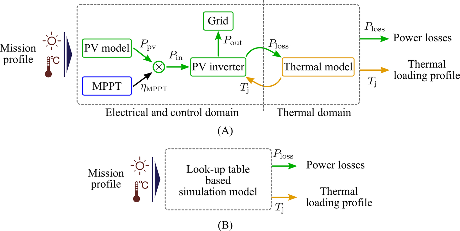
From the given mission profile, the PV power production (Ppv) can be determined by using the PV panel electrical characteristic model. Then, the actual input power seen by the PV inverter (Pin) is obtained by taking the MPPT algorithm efficiency (ηMPPT) into account. In order to estimate the power losses in the power devices (Ploss), a PV inverter loss model is employed. This can be obtained by considering the switching losses and conduction losses of the power devices in the inverter. After that, the thermal model of the power devices can be applied in order to obtain the junction temperature profile of the power devices (Tj) during the entire operation, which is implemented by using an LUT, as mentioned previously, in order to enable a long-term mission profile translation (e.g., yearly mission profiles) [59]. Fig. 45.17 summarizes the above process.
As an example (for the 600 V/30 A device), one of the translated thermal loading profiles under the mission profile (Figs. 45.11 and 45.12) is shown in Fig. 45.18. The cycle amplitude (△Tj) and the mean junction temperature (Tjm) are presented in Fig. 45.18A and B, respectively. The impact of the mission profile can be observed in Fig. 45.18 from the thermal loading of the power device, where the cycle amplitude profile follows the variation in the solar irradiance profile (i.e., part of the mission profile). The long-term variation in the mean junction temperature has the similar tendency as the ambient temperature profile in Fig. 45.12 with a short-term variation imposed by the variation in the solar irradiance profile in Fig. 45.11.

45.4.2 Thermal Loading Interpretation
The junction temperature profile shown in Fig. 45.18 reflects the impact of mission profiles on the thermal loading of the power electronic system. However, it provides limited qualitative information about the thermal loading of the power devices, as the cycle amplitude (△Tj) and the mean value of the junction temperature (Tjm) are an irregular profile due to the mission profile dynamics. In other words, it cannot be directly applied to an empirical lifetime model. Thus, a cycle-counting algorithm such as rainflow analysis is normally employed in order to divide the irregular profile into several regular thermal cycles [52]. With this analysis, the qualitative information such as the number of cycles ni at a certain cycle amplitude △Tj, mean junction temperature Tjm, and cycle period ton can be obtained and applied to the lifetime model. Details of the rainflow algorithm can be found in [30,60,61].
45.4.3 Lifetime Model of Power Devices
The lifetime model of the interested power component is required for the lifetime prediction. In the case study, the lifetime of the power electronic systems (devices) is considered. Several lifetime models of the power electronic devices, components, or modules have been developed. A recently developed IGBT lifetime model that considers the thermal cycle period ton is adopted [53], and it is expressed as

where Nf, △Tj, Tjm, and ton are defined previously. The other parameters are constants that are given in Table 45.1. Using the interpreted thermal loading information and (45.4), the LC of the power electronic components can be obtained according to (45.2). When the LC is accumulated to unity, the power electronic device reaches its end of life, as mentioned previously.
Table 45.1
Parameters of the lifetime model of an IGBT module [53]
| Parameter | Value | Experimental Condition |
| A | 3.4368×10¹⁴ | |
| α | −4.923 | 64≤△Tj≤113 K |
| β1 | −9.012×10⁻³ | |
| β0 | 1.942 | 0.19≤ar≤0.42 |
| C | 1.434 | |
| γ | −1.208 | 0.07≤ton≤63 s |
| fd | 0.6204 | |
| Ea | 0.06606 eV | 32.5≤Tj≤122 °C |
| kB | 8.6173324×10⁻⁵ eV/K |
45.4.4 Monte Carlo Reliability Assessment
The reliability metric is usually expressed in terms of statistical values, rather than a fixed value obtained previously, due to the uncertainties in the lifetime prediction. The uncertainties can be introduced by the component-parametric variations (e.g., due to the manufacturing process), lifetime- parametric variations (e.g., due to the test data), and variations in the stresses (e.g., variations in the PV power production due to the PV panel aging). In order to include the impact of those uncertainties into the lifetime prediction, a Monte Carlo analysis is employed [26,62], according to the flow shown in Fig. 45.16.
In the Monte Carlo analysis, variations are introduced to the lifetime model of (45.4) and also the stressors, where the parameters can be modeled with a certain distribution function (e.g., a normal distribution), as illustrated in Fig. 45.19. Following the Monte Carlo approach, a large set of populations are taken randomly from the distribution in Fig. 45.19 and applied to the lifetime model. Therefore, the lifetime distribution (or time-to-failure distribution) can be obtained and fitted with a specific distribution function. Normally, the lifetime distribution of the wear-out failure follows the Weibull distribution, and the Weibull probability density function (Weibull PDF) is shown in Fig. 45.20A. Notably, it is also possible to analyze the influence of an individual parametric variation by using the sensitivity study. This can be used for identifying the crucial parameter that limits the lifetime of the component (which may be redesigned). For instance, a controlled cooling unit may be required, if the lifetime is sensitive to the mean junction temperature.


From the lifetime distribution (i.e., the Weibull PDF), the reliability of one single power device (e.g., component level) can be determined by considering the CDF of the lifetime distribution. The Weibull CDF distribution (Weibull CDF) shown in Fig. 45.20B is referred to as the unreliability function, as it represents the percentage of failure population overtime. The Bx lifetime can be obtained from the unreliability function. For instance, the B1 and B10 lifetime of the power device, which indicates the time when 1% and 10% of the population have failed, are the commonly used reliability metrics.
45.4.5 System-Level Reliability Analysis
In many cases, the system under consideration consists of several components, where each component has its own unreliability function. The Bx lifetime of one single component may not accurately reflect the Bx lifetime of the overall power electronic system. Thus, the system-level reliability assessment is performed using the reliability block diagram. For the full-bridge PV inverter shown in Fig. 45.7, the system-level reliability block diagram consists of a series connection of four components, as the failure of any power device (e.g., S1, S2, S3, or S4) will lead to the loss of functionality of the entire power electronic system. Thus, according to (45.3), the system-level unreliability function can be calculated as
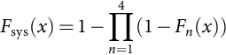
where Fsys(x) is the system-level unreliability function and Fn(x) is the component-level unreliability function of the n-th component. The system-level unreliability function of the PV inverter (e.g., four devices) is shown in Fig. 45.20B, where it can be noticed that the system-level unreliability is in general higher than the component-level unreliability (i.e., Fsys(x)≥Fn(x)), resulting in the lower Bx lifetime for the system level.
45.4.6 Design for Reliability (DfR) Results
The reliability analysis is carried out with three selected power devices following the above. As specified in the reliability target, the system-level lifetime of the PV power electronic system should be higher than 25 years. This is the benchmark for selecting the most suitable power electronic device among the three candidates. The DfR results are shown in Fig. 45.21. The lifetime distribution of each device obtained from the Monte Carlo analysis is shown in Fig. 45.21A, where it can be seen that the lifetime distribution of the three power electronic devices shows significant difference. A majority of the population with the 15-A power devices fail after 10 years of operation, while most of the population with the 30- and 50-A power devices can survive after 100 and 250 years of operation, respectively. However, it should be noted that in such cases other parameters will determine the lifetime. Additionally, the ratings of the two devices are over designed compared with the rating of the system under study (i.e., 6-kW). Both lead to the relatively long lifetime.

Based on the lifetime distribution in Fig. 45.21A, the unreliability function can be obtained, as it is shown in Fig. 45.21B, where the Bx lifetime is also indicated. For example, it can be seen from Fig. 45.21B that the system-level B1 lifetime of the PV inverter is 2 years if the 15-A power devices are selected. This means that the power electronic system with 15-A power devices did not meet the reliability target of 25 years under the given mission profile. On the other hand, the PV inverter with 30- and 50-A power devices has the system-level B1 lifetime of 30 and 61 years, respectively. Therefore, either the 30- or 50-A power device can be used in the full-bridge power electronic system that fulfills the reliability target. In most cases, the cost of the power devices with the current rating of 30 A will be lower than that of the 50-A power devices. Thus, the 30-A power electronic device is considered to be the most suitable candidate to be used in the PV power system in order to achieve the system-level B1 lifetime higher than 25 years. However, it is also worth mentioning that the predicted lifetime is relatively long, since there are many other factors influencing the reliability. In this case study, only the failure mechanism related the junction temperature is considered. To improve the reliability prediction, more failure mechanisms as well as possible coupling effects should be taken into account. It in return may make the analysis become more complicated. Nevertheless, the above demonstrates a way to lifetime prediction, and thus enables the DfR in power electronic systems.
45.5 Summary
The reliability demands for power electronic systems have been identified in this chapter. The state of the art in power electronic converters for wind and PV power systems have been briefly reviewed, from which it is known that the power electronic systems play a vital role in the power conversion. The conventional design of power electronic systems focuses on power density and efficiency. However, the power electronic system is also one of the most life-limiting parts, and thus, the reliability should be included in the design phase, being the design for reliability (DfR) approach, as demonstrated in this chapter. Multidisciplinary efforts in component physics, reliability engineering, system engineering, and power electronics are necessary to implement the DfR approach. Many challenges still exit in mission profile modeling, lifetime modeling, reliability data in software, human errors, single-event catastrophic failures, and reliability-oriented design tools as discussed in [20]. Other relevant studies related to this chapter have been collectively presented in [63], which provides an overview of the recent advancements in the area of reliability of power electronic converter systems and also reliability testing.