
Electric Power Transmission
Muhammad H. Rashid University of West Florida, Pensacola, FL, United States
Zahrul F. Hussien Transmission and Distribution TNB Research, Kajang, Malaysia
Azlan A. Rahim Transmission and Distribution TNB Research, Kajang, Malaysia
Norazlina Abdullah Transmission and Distribution TNB Research, Kajang, Malaysia
Abstract
Modern electric power system consists of complex interconnected network of components. This chapter covers the components that make up the modern power system. These include generators, transformers, and transmission line. It also focuses on the transmission of electric power, how to optimize its power transfer capability, the phenomena of over-voltages and the insulation requirement of transmission lines.
Keywords
Thermal rating; ACSR; Overvoltage; Transmission line; HVDC; Transmission loss; Conductor sag; Optimizing; Insulation; Switching surges
26.1 Elements of Power System
The growth of electricity production and usage in the world is at an all-time high. It is the fastest growing form of end-use energy worldwide. The world net electricity generation in the year 2006 is estimated at 18 trillion kWh. It is forecasted to be 23.2 trillion kWh in the year 2015 and 31.8 trillion in the year 2030 [1]. Electricity production from fossil fuels raises concern on climate change, and hence, alternative energy sources such as solar, geothermal, wind, wave, tidal, and biomass are being developed rapidly around the world.
Modern electric power system consists of complex interconnected network of components generally divided into generation, transmission, distribution, and load. The invention of the transformer at the end of the nineteenth century enables electric energy to be transmitted at higher voltages and hence higher capacity. In this chapter, the components that make up the modern power system are briefly reviewed, namely, generators, transformers, and transmission line. The chapter will focus on the transmission of electric power and how to optimize its power transfer capability. The chapter will also discuss the phenomena of overvoltages and the insulation requirement of transmission lines. The use of power electronics in electric power transmission is covered in Chapters 31 and 32, respectively, such as high-voltage direct current (HVDC) system and flexible AC transmission system (FACTS) (Fig. 26.1).

26.2 Generators and Transformers
Generators are the starting point in a power system where electricity is generated. The most commonly used type of generator is the synchronous generator, driven by a prime mover. In a thermal power station, the prime mover is powered by steam turbines using coal, gas, nuclear, or oil as the fuel. Steam turbines usually operate at high speed to optimize its power output. For a 60 Hz system, the speed of rotation is 3600 (two-pole machine) or 1800 rpm (four-pole machine). For a 50 Hz system, the speed of rotation is 3000 (two-pole machine) or 1500 rpm (four-pole machine). Hydropower station uses the potential energy of water to power the hydraulic turbines. The hydraulic turbines usually operate at relatively low speed, coupled to generators with salient-type rotor with many poles. In power-generating stations, the electric power is generated at high voltages typically between 10 and 30 kV, while the size of the generators varies from 50 to 1500 MW (Fig. 26.2).
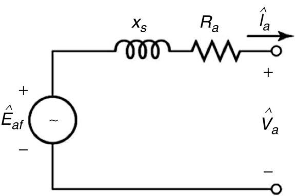
A synchronous generator produces alternating current in the armature winding (usually a three-phase winding on the stator) with dc excitation supplied to the field winding (usually on the rotor). The per-phase equivalent circuit of a synchronous generator is shown below where the armature voltage, Va, can be written as
where
Ra is the armature resistance
Ia is the armature current
Xs is the synchronous reactance
Eaf is the internal generated voltage
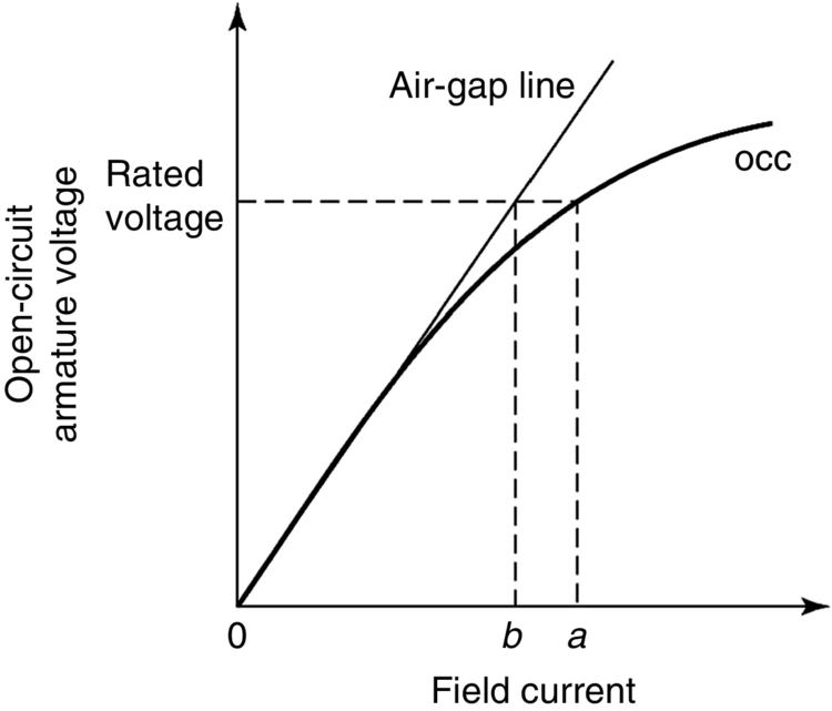
The open-circuit characteristic (occ) of a synchronous generator as shown below represents the relationship between the field current If and the internal generated voltage Eaf. Note that with the armature winding open-circuited, the armature voltage Va is equal to the internal generated voltage Eaf. As the field current If is increased from zero, the armature voltage Va increases linearly. Near the rated voltage, the saturation effect is clearly seen with the departure of the occ from the straight line (air-gap line) (Fig. 26.3).
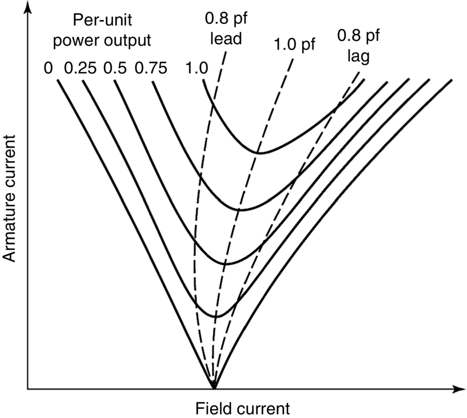
Another characteristic of the synchronous generator is illustrated by the V curve shown in Fig. 26.4. For a constant real-power loading, the field current and hence excitation can be adjusted to vary the reactive power VAr generated, hence power factor (pf).
The voltage output of the generator is transformed to a higher voltage before transmitting the power over a long distance to reduce the transmission losses, I2R losses. Transformers are used to step up or step down the voltage (Fig. 26.5).
Transmission system voltages vary from country to country. For example, in Britain, they are 400 and 275 kV; in the United States, they are 765, 500, and 345 kV, while in Malaysia, they are 500 and 275 kV. The subtransmission network is at 115 kV in the United States, while it is 132 kV in Britain and Malaysia. This network in turn supplies the distribution network to the customers in a given area. In Britain and Malaysia, the distribution network operates at 33 and 11 kV supplying the customer's feeders at 400 V three-phase and 230 V per-phase. Transformer used in the power system ranges from small 500 kVA distribution transformers to 1000 MVA supergrid transformers.
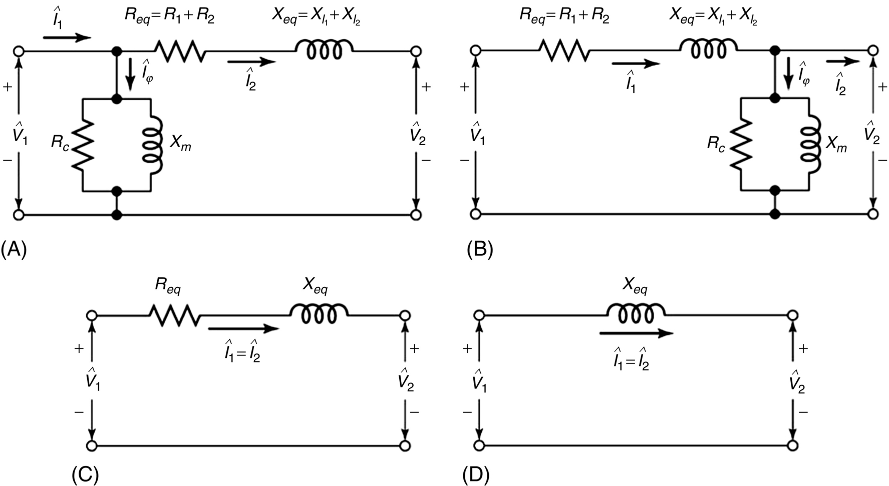
Detailed theoretical analysis of transformers has been covered in numerous textbooks. It is suffice to show here the equivalent circuit of a transformer to appreciate its electric circuit representation. The component Rc represents the core losses that consist of eddy current losses and hysteresis losses, while the component Xm represents the flow of the magnetization current. Core losses also known as no-load losses are essentially the power required to energize the core. It depends primarily on the voltage and frequency and does not vary much with system operation variations. On the other hand, Req and Xeq represent the primary and secondary winding of the transformer where the load losses originate. Load losses consist of the I2R losses mainly in the windings and stray losses that include winding eddy losses and the effect of leakage flux entering internal metallic structures (Fig. 26.6).
26.3 Transmission Line
The bulk transfer of electric energy from generating power plants to substations located near population centers is achieved through high-voltage transmission lines. Interconnected transmission lines are referred to as high-voltage transmission networks. Electricity is transmitted at high voltage to reduce the energy lost in long-distance transmission. It is important to understand the characteristic of the important component, which is the conductor, to appreciate the limiting factors to the power transfer capability of the transmission line. The power transfer can then be optimized using latest sensor and communication technology.
The conductor is one of the major components of a transmission line design. It is essential that the most appropriate conductor type and size be selected for optimum operating efficiency. There are four common types of conductors used for many years in electric utilities: (i) all-aluminum conductor (AAC), (ii) aluminum conductor steel reinforced (ACSR), (iii) aluminum conductor alloy reinforced (ACAR), and (iv) all-aluminum alloy conductor (AAAC). Regardless of the type of metal used in the makeup of the conductor, the strands are always round and have a concentric lay.
26.3.1 Aluminum Conductor Steel-Reinforced
Electric utility companies have utilized ACSR as a common choice of conductor in transmission lines for many years. ACSR is used extensively on long spans as both ground and phase conductors because of its high mechanical strength-to-weight ratio and good current-carrying capacity. ACSR consists of solid or stranded coated steel core surrounded by one or more layers of 1350-H19 aluminum. Because of the presence of the 1350 aluminum in the construction, ACSR has equivalent or higher thermal ratings to equivalent sizes of AAC [2] (Fig. 26.7).
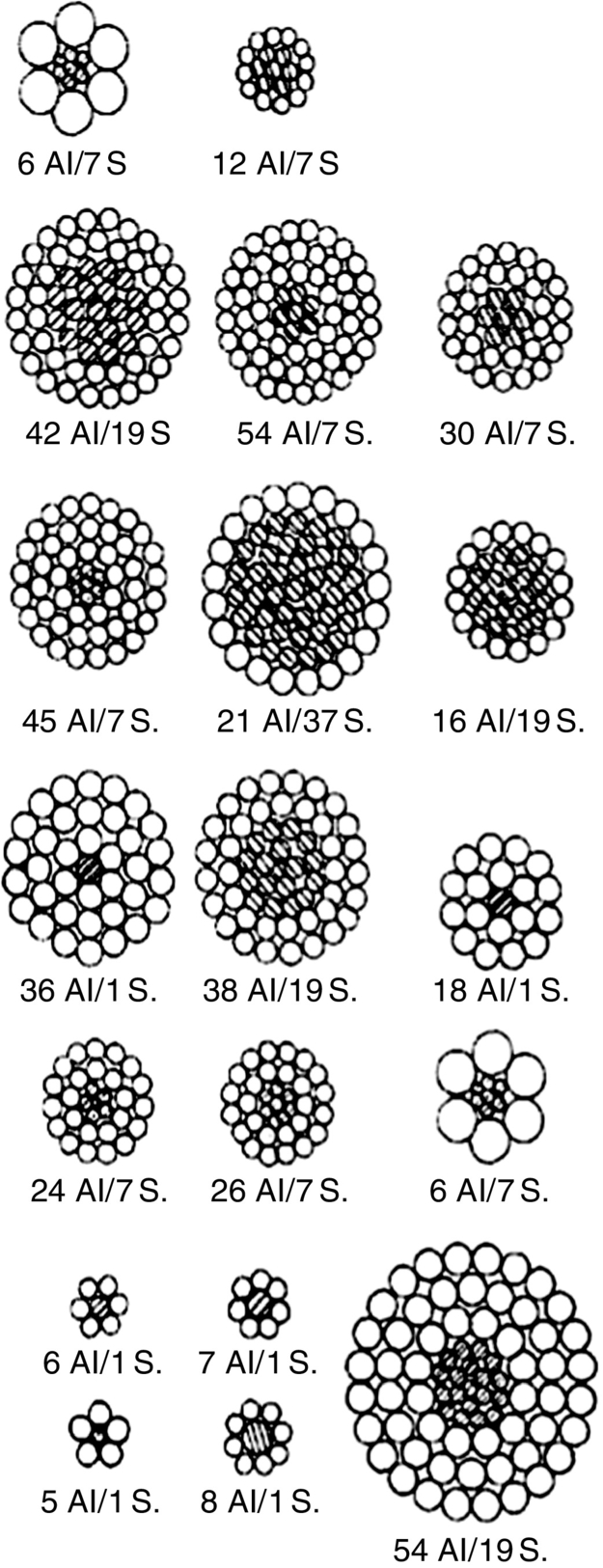
The cross-sectional area of ACSR is specified according to the cross-sectional area of aluminum to be contained in the construction. For example, a 428 mm2 54/7 ACSR has 428 mm2 of aluminum, the equivalent aluminum area content of 428 mm2 AAC. The steel content of ACSR typically ranges from 11% to 18% by weight for the conductor stranding of 18/1, 45/7, 72/7, or 84/19. However, it can vary up to 40% depending on the desired tensile strength. It is desirable for ground wires in extra-long spans crossing rivers, for example, to have a stranding of 8/1, 12/7, or 16/19, giving them higher tensile strength. Fig. 26.8 shows the standard stranding of ACSR [3].
The high tensile strength combined with the good conductivity gives ACSR several advantages such as the following:
• The high tensile strength of ACSR allows it to be installed in areas subject to extreme wind loading.
• Because of the presence of the steel core, lines designed with ACSR elongate less than other standard conductors, yielding less sag at a given tension. Therefore, the maximum allowable conductor temperature can be increased to allow a higher thermal rating when replacing other standard conductors with ACSR.
• ACSR is less likely to be broken by falling tree limbs.
26.4 Factors That Limit Power Transfer in Transmission Line
Factors that limit the power transfer are voltage drop, voltage stability, and thermal rating. For short transmission line, which is approximately less than 80 km, the power transfer is limited by the thermal rating. The thermal rating is limited by the maximum operating temperature of the conductor. This maximum operating temperature is limited by the maximum line sag limit and maximum allowable operating temperature of the conductor material.
26.4.1 Static and Dynamic Thermal Rating
Static thermal rating of the overhead transmission line is a fix rating in terms of current-carrying capacity. It is a conservative rating where worse case weather for contributing for maximum heat onto the conductor is assumed.
Dynamic thermal rating of the overhead transmission line is a time-dependence rating where the actual weather and loading of the conductor are measured and the thermal rating is calculated in real time.
26.4.2 Thermal Rating
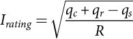
Bare overhead conductor is normally exposed to environment when it is in service. Due to this reason, the conductor temperature is normally influenced by weather condition and the electric current loading of the conductor. In thermal rating calculation, meteorologic parameters such as wind speed and direction, solar radiation, and ambient temperature are required for the calculation where the calculation is based on heat balance energy equation; in steady-state condition, the conductor heat gain is equal to the heat loss (no heat energy is stored in the conductor). The mathematical representation of the heat balance energy equation as in Eq. (26.1) and by reorganizing the equation as in Eq. (26.2), the thermal rating can be calculated [4]. The heating elements are solar radiation and internal heating by the electric current flow through the conductor resistance or ohmic loss (I2R). The heat loss is due to convection and radiation:
where
qs heat input due to solar, W/m
I2R(Tc) heat input due to line current (R is a function of conductor temperature)
qc heat output due to convection (a function of wind, air temperature, and conductor temperature), W/m
qr heat output due to radiation (a function of wind, air temperature, and conductor temperature), W/m
26.4.3 Convection Heat Loss
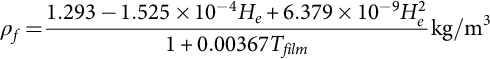
Convection heat-loss calculation can be grouped into natural convection and forced convection. The natural convection heat loss, qcn, is calculated in the condition where there is no wind. This happens in all thermal systems where there is a thermal gradient. Heat will migrate from the hotter region to the cooler region until the temperature is uniform across the entire system. The natural convection heat loss (watt per unit length, W/m) for the bare-stranded overhead conductor is a function of air density, ρf; conductor diameter, D; and temperature difference between conductor and ambient, ![]() , as given by Eq. (26.3) [4]:
, as given by Eq. (26.3) [4]:
In conditions where there is wind, wind blowing against the bare overhead conductor introduces cooling effect where the heat from the conductor will be transferred over the temperature gradient, from high to low, to the moving air; this is called forced convection heat loss. There are two equations used in the calculation for the forced convection heat loss. One is used for low wind speed, qc1, and another for high wind speed, qc2 [4]. The reason that there are two similar, yet independent, equations is because the correction factors incorporated into the equations are proprietary to a certain band of conditions. Eq. (26.4) is for low wind speed, and Eq. (26.5) is for high wind speed:


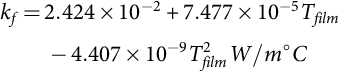
where air density, ρf; air viscosity, μf; and coefficient of thermal conductivity of air, kf, are calculated using Eqs. (26.8), (26.9), and (26.10), respectively, at Tfilm where
At any wind speed, the highest of the two calculated forced convection heat-loss rates is used. The angle at which the wind is blowing relative to the conductor's axis is also considered. The convective heat-loss rate is multiplied by the wind direction factor, Kangle, where ϕ is the angle between the wind direction and the conductor axis. This modifying factor is used to create a modified forced convective heat-loss value. The maximum heat loss will occur when the wind is perfectly perpendicular. The wind direction factor is calculated using Eq. (26.7):

26.4.4 Radiative Heat Loss
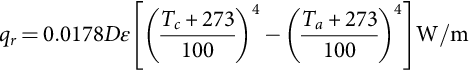
Radiative heat loss is usually a small fraction of the total heat loss. It is depending on conductor diameter, D; emissivity, ɛ; conductor temperature, Tc; and ambient temperature, Ta, as given by Eq. (26.11) [4]. If the ambient temperature is kept constant, for example, at ![]() , the radiative heat loss increases exponentially with conductor temperature as shown in Fig. 26.9. Emissivity, ɛ, is dependent on the conductor surface and varies from 0.27 for new stranded conductor to 0.95 for industrial weathered conductors [5]. It is equal to the ratio of the heat radiated by the conductor and to the heat radiated by a perfect blackbody of the same shape and orientation. Typical values for new bare overhead conductor are between 0.2 and 0.3. The solar emissivity of a new bare overhead conductor increases with age. A typical value for a conductor that has been in use for more than 5 (in industrial environments) to 20 years (in rural clean environments) is 0.7. A value of 0.5 is used if nothing is known about the conductor emissivity [4]:
, the radiative heat loss increases exponentially with conductor temperature as shown in Fig. 26.9. Emissivity, ɛ, is dependent on the conductor surface and varies from 0.27 for new stranded conductor to 0.95 for industrial weathered conductors [5]. It is equal to the ratio of the heat radiated by the conductor and to the heat radiated by a perfect blackbody of the same shape and orientation. Typical values for new bare overhead conductor are between 0.2 and 0.3. The solar emissivity of a new bare overhead conductor increases with age. A typical value for a conductor that has been in use for more than 5 (in industrial environments) to 20 years (in rural clean environments) is 0.7. A value of 0.5 is used if nothing is known about the conductor emissivity [4]:

26.4.5 Solar Heat Gain
The solar heat gain, qs, depends on the conductor diameter, D; absorptivity, α; and global solar radiation, S, as given by Eq. (26.12):
The conductor solar absorptivity, α, is a number that varies between 0.27 for bright stranded aluminum conductor and 0.95 for weathered conductor in industrial environment. It is equal to the ratio of the solar heat absorbed by the conductor to the solar heat absorbed by a perfect blackbody of the same shape orientation. Typical values for new conductor are between 0.2 and 0.3. The solar absorptivity of an overhead conductor increases with age. A typical value for a conductor that has been in use for more than 5 (in industrial environments) to 20 years (in rural clean environment) is 0.9. A value of 0.5 is often used if nothing is known about the conductor absorptivity [4].
26.4.6 Ohmic Losses (I2R(Tc)) Heat Gain
The ohmic loss of the bare overhead conductor is depending on the amount of current flows and conductor electric resistance, whereas the conductor electric resistance is depending on conductor temperature. For all bare overhead conductors, controlled lab tests have been carried out; high and low temperature and electric resistance values have been established. This is then published as a guide for electric utilities to use as a reference in their estimation of their system's performance. As upper and lower limits have been defined, it is merely a matter of interpolation to obtain values between the given temperatures. For values outside the envelope, extrapolation can be readily used to obtain the result with reasonable accuracy. For example, lab tests conducted for 1350-H19 aluminum show that for entry resistance values at temperatures of 25°C and 75°C, the errors are negligible [6]. For entry resistance values at temperatures of 25°C and 175°C, the errors are approximately 3% too low at 500°C but 0.5% too high at 75°C. It is concluded that the use of resistance data for temperatures of 25°C and 75°C is adequate for rough calculation of steady-state and transient thermal rating for conductor temperature up to 175°C. The formula that is used to obtain the resistance of the conductor, per unit length, based on the established lab test results is given in Eq. (26.13):
26.5 Effect of Temperature on Conductor Sag or Tension
26.5.1 Conductor Temperature and Sag Relationship
The relationship of the sag to the temperature of a homogenous conductor is almost linear. A third-degree equation gives a very close approximation of the temperature as a function of the sag, Eq. (26.14) [7]:
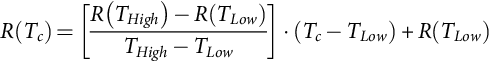
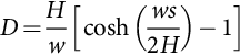
The line sag can be determined from the measured tension or direct measured ground clearance. For practical purposes, the sag can be considered to be inversely proportional to the tension in most spans. For a higher degree of accuracy, the sag/tension relationship can be determined to any desired degree of accuracy based on catenary equations. For level conductor spans as in Fig. 26.10, the low point is in the center of the total sag, D, given by Eq. (26.15):

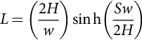
The horizontal component of tension, H, is located at the point in the span where the conductor slope is horizontal or at the midpoint for level spans. The conductor tension, T, is found at the ends of the spans at the point of attachment and is calculated using Eq. (26.16), and it corresponds to a conductor length, L, given by Eq. (26.17):
Eq. (26.17) describes the behavior of ideal (with perfectly elastic stress and strain characteristics) concentric-lay-stranded conductors [6]. The actual conductors such as ACSR conductors exhibit nonlinear behavior when loaded from initial tension to some final value due to wind or temperature loading. Permanent elongation from creep and heavy loading also affects the resulting sag. Also, high-temperature operations result in thermal elongation of the steel and aluminum strands, thus affecting sag. Therefore, in order to calculate the correct sag, it is necessary to separate the effects of conductor elongation due to tensile loading and thermal loading. This process requires an iterative procedure in which the mathematical formulas describing the conductor elongation caused by the temperature change are solved simultaneously with the tension and conductor length relationship. To calculate the change in length due to temperature loading, Eq. (26.18) is used:
where
![]() =reference length of the conductor
=reference length of the conductor
αAS=coefficient of linear thermal elongation for AL/SW strands, given in Table 26.1
Table 26.1
Coefficients of thermal expansion for bare-stranded conductors [8]
| Conductor | α (per °C) |
| AAC | |
| 36/1 ACSR | |
| 18/1 ACSR | |
| 45/7 ACSR | |
| 54/7 ACSR | |
| 26/1 ACSR | |
| 30/7 or 30/19 ACSR |
![]() =change in temperature
=change in temperature
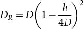
For inclined spans, the length of the conductor between the supports is divided into two separate sections as in Fig. 26.11. The same equation in (26.15) can be used for the calculation of the height of the conductor. In each part of the span, the sag is dependent upon the vertical distance between support points and can be described by Eqs. (26.19) and (26.20) [7]:
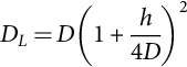
Most of the sag and tension calculations are typically performed with line rating software, for example, PLS-CADD software from Power Line Systems, Inc., the Unites States. To demonstrate the process on how sags and tensions occur for overhead line, simplified sag calculations and conductor length can be done by using Eqs. (26.21) and (26.22), respectively [6]:
The example of the relationship between conductor temperature and conductor sag can be describe by the following example [8].
A transmission line with ACSR conductor 795 kcmil (405 mm2) and a 1000 ft level span. The conductor weight per unit length is 1.094 lb/ft (1.6 kg/m), ambient temperature is 77°F (25°C), and horizontal tension component, H, is 25% of the ultimate tension strength (31,500 lb):
Conductor sag, D, is calculated by using Eq. (26.21):

Conductor length, L, is calculated by using Eq. (26.22):
Eq. (26.18) is used to calculate the conductor length when the conductor temperature increases from ambient to 50°C (122°F) and then to 150°C (302°F). The coefficient of linear thermal expansion is ![]() :
:
The conductor sag is calculated by rearranging Eq. (26.22):
The relationship of the conductor temperature and the conductor sag for the above example can be summarized in Table 26.2.
Table 26.2
Relationship between conductor temperature and conductor sag for the ACSR conductor 405 mm2 for a 1000 ft level span [6]
| Conductor temperature (°C) | Conductor sag, D (m) |
| 25 | 5.29 |
| 50 | 6.68 |
| 150 | 10.58 |
The conductor temperature corresponds to the measured sag given by Eq. (26.14), since the current conductor temperature is known; the dynamic thermal rating for the maximum conductor temperature, for example, at 75°C can be calculated by using Eq. (26.2).
From the known conductor temperature, the value of qr can be calculated by the thermal rating Eq. (26.11). The value of qs can be calculated by Eq. (26.12); the conductor resistance at the known temperature can be calculated by Eq. (26.13). By rearranging the thermal balance equation and with the known value of conductor current, the convective heat loss qc can be calculated using Eq. (26.23):
From the known value of qc, the equivalent perpendicular wind speed can be calculated by Eq. (26.4) or (26.5). Assuming the equivalent perpendicular wind speed is constant, then the thermal rating at the maximum conductor temperature can be calculated.
26.6 Standard and Guidelines on Thermal Rating Calculation
Reference standard for thermal rating calculation is published by IEEE; the first standard is IEEE Std 738-1993, IEEE Standard for Calculation of Bare Overhead Conductor Temperature and Ampacity Under Steady-State Conditions. Later, the new revision of this standard is published, IEEE Std 738-2006. The revised standard has additional information that addresses fault current and transient rating calculation, SI units were used throughout, and the solar heating calculation was extensively revised to cater for most part of the world instead of only 20 degrees north and above in the first standard IEEE Std 738-1993. The IEEE standard presents a method of calculating the current-temperature relationship of overhead lines given the weather conditions. The heat balance energy equation used for thermal rating calculation is described in details in this standard. The equation relating electric current to conductor temperature described in this standard can be used in two ways:
• To calculate the conductor temperature when the electric current is known
• To calculate the current that yields a given maximum allowable conductor temperature
Other guidelines on thermal rating calculation were developed by CIGRE working group WG 22.12, published in Electra No. 144 in October 1992, The thermal behavior of overhead conductors, Sections 1 and 2: Mathematical model for evaluation of conductor temperature in the steady state and the application thereof. And another one was published in Electra No. 174 in October 1997, The thermal behavior of overhead conductors, Section 3: Mathematical model for evaluation of conductor temperature in the unsteady state. In these guidelines, the heat balance energy equation is discussed in more details compared with in IEEE standard where other addition elements are added in the heat balance energy equation such as magnetic heating, corona heating, and evaporating cooling.
26.7 Optimizing Power Transmission Capacity
26.7.1 Overview of Dynamic Thermal Current Rating of Transmission Line
Real-time thermal rating methods can be classified into two basic types: weather model (WM) and conductor temperature model (CTM) [4]. The difference between the two models is the method by which the conductor convective heat-transfer coefficient is calculated. The WM approach calculates the convective heat-transfer coefficient using ambient temperature, wind speed, and wind direction data together with empirical expressions for convective heat transfer for airflow past cylindrical objects. The CTM computes the convective heat-transfer coefficient directly using the conductor heat balance energy equation, conductor temperature, air temperature, and conductor current. There are five main dynamic thermal rating techniques in WM and CTM, that is, weather monitoring, line tension monitoring, sag monitoring, line temperature monitoring, and conductor replica technique. The most appropriate technique depends upon a particular application and is based on various issues including accuracy, cost, and ease of installation [8].
In general, the overview of DTCR system is as shown in Fig. 26.12. There are three main components that form the dynamic thermal current rating (DTCR) system: remote monitoring station, communication system, and the system computer. Remote monitoring station gathers information on the environment in which the transmission lines are located and also information on the line sag/clearance or tension or conductor temperature. The remote monitoring station is normally placed at a critical location along the transmission line where the wind cooling is minimal or where there is an increased probability of contact between the conductor and objects on the ground.

The communication system used in this real-time thermal rating system can be wireless or wired system. Normally, wireless communication system is more suitable for the thermal rating system compared with wired system due to connectivity issues and cost. The wireless system is easy to be implemented; it is robust and suitable for use in the outdoor environment. Data transfer from the remote monitoring station to the system computer can be based on dial-up connection at certain time intervals.
The system computer normally consists of two software modules, thermal rating calculation module and thermal rating display module. It has two primary functions, namely, to process the weather and line clearance data then calculate the thermal rating of the line and to display the thermal rating in real time.
As electric current in an overhead conductor increases, the line temperature increases, and therefore, the line sags. Each line has a minimum clearance to ground, which must never be violated for safety reasons. The thermal rating is the maximum current that results in the line sagging down exactly to the minimum clearance. Any additional current would result in too much sag and therefore breaches the safety requirement [9].
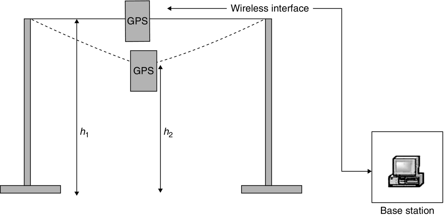
There are a few methods of transmission line sag monitoring that has been developed. One of the methods proposed is based on global positioning system (GPS). The method is known as differential GPS [10]. This mode consists of the use of two GPS receivers, the base and the rover as shown in Fig. 26.13. The actual position of the base is known (e.g., by precise surveying) and compared with the readings received at the same base point. With the estimated error, the readings obtained at the rover can be compensated by simple subtraction.
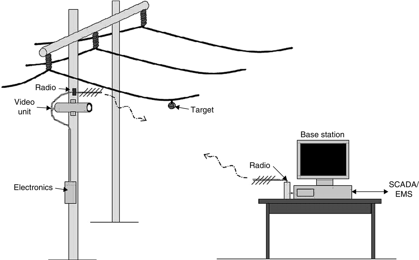
Another method to monitor the line sag is by using smart camera. This method is developed by Electric Power Research Institute (EPRI), the United States [4]. The system uses an imaging system to monitor the location of the conductor or a target attached to it as shown in Fig. 26.14. The imaging system is installed on either a transmission line structure or any other structure with a view of the span being monitored. The field of view of the imaging system remains the same at all time, and the location of the conductor or the target in the view changes as the conductor moves up, down, or horizontally. Image-processing technique is used to determine the location of the conductor or the target attached to the conductor in the camera's field of view. The search algorithm uses a preselected subimage of the target and searches the image to determine the most likely location of the target in the camera image. The key for the success of this approach is to have a target with unique features that cannot be easily found in the background. The change in vertical position of the conductor in the image is directly related to the change in ground clearance or sag. At the time of installation, location of the conductor or the target attached to the conductor in the imaging system's field of view is calibrated to the measured ground clearance/sag. Ground clearance or sag at any later time is obtained from the measured change in location of the conductor using calibration constants obtained at the time of system calibration. The resulting clearance information may be made available on a real-time basis using telemetry and/or logged in a data logger for historical study. An effective conductor temperature is calculated using sag-tension routines of line rating software such as PLS-CADD software from Power Line Systems, Inc., the United States, and the real-time ratings is calculated using IEEE standard 738 [4].
Tension monitors consist of solar-powered line tension monitoring system located along the transmission line that communicate the measured data via spread-spectrum radios to receiving units at substations that are further linked to the utility's EMS/SCADA systems. The conductor tension is measured using load cell installed at the dead-end insulators. There are also sensors that measure the ambient temperature and the net radiation at the conductor. All data are transmitted to the center processor computer for the line thermal rating calculation. The calibration of the system allows determination of the conductor temperature based on the measured tension [2].
Direct measurement of conductor temperature method uses temperature sensor that is directly attached to the conductor. It uses solid-state thermoelectric sensors, and it is powered up using line-current transformer. The system was developed by Niagara Mohawk in the 1980s, and the temperature sensor was called Power Donut. This method can provide conductor temperature data in real time. Power Donut has ambient and conductor temperature measurement accuracy of ![]() over a range of −40°C to 125°C [12]. The advantage of this method is that the user has a direct measurement of conductor temperature. If the line rating is intended to limit the loss of conductor strength at high temperature, then this method is mostly appropriate.
over a range of −40°C to 125°C [12]. The advantage of this method is that the user has a direct measurement of conductor temperature. If the line rating is intended to limit the loss of conductor strength at high temperature, then this method is mostly appropriate.
Ground clearance has direct relationship with line sag as they depend on conductor temperature. Therefore, thermal rating can also be determined by monitoring the ground clearance. Laser distance measurement sensor can be used to measure the distance between the transmission line and ground. The installation of the laser distance measurement sensor must be at the middle of the span on the ground directly under the transmission line as shown in Fig. 26.15.

To enable continuous monitoring of the line clearance, the sensor can be set to operate in automatic mode that will take measurement continuously for a certain time interval. The line thermal rating can be calculated based on the conductor temperature determined by the clearance measurement.
A number of studies have shown that it is possible to calculate the thermal rating of an overhead conductor in a single span if the weather conditions in the span are known. This can be done using historical weather data records in order to select appropriately conservative static ratings, or it can be done in real time as a basis to dynamically rate the line. By accounting for variations in span orientation along a transmission line, it was found that the weather data from a single weather station as far as 20 mi away could be used to predict the statistical distribution of thermal ratings for that line [5]. For a real-time monitoring, the dynamic thermal rating of the line is calculated using real-time value of the line load current and the weather data. Example of a weather station installation at the transmission line is shown in Fig. 26.16.

26.7.2 Example of Dynamic Thermal Current Rating of Transmission Line
The dynamic rating profile as shown in Fig. 26.17 is based on DTCR calculations using weather data recorded by a weather station for one of the transmission lines in Malaysia [13]. The figure shows three curves:
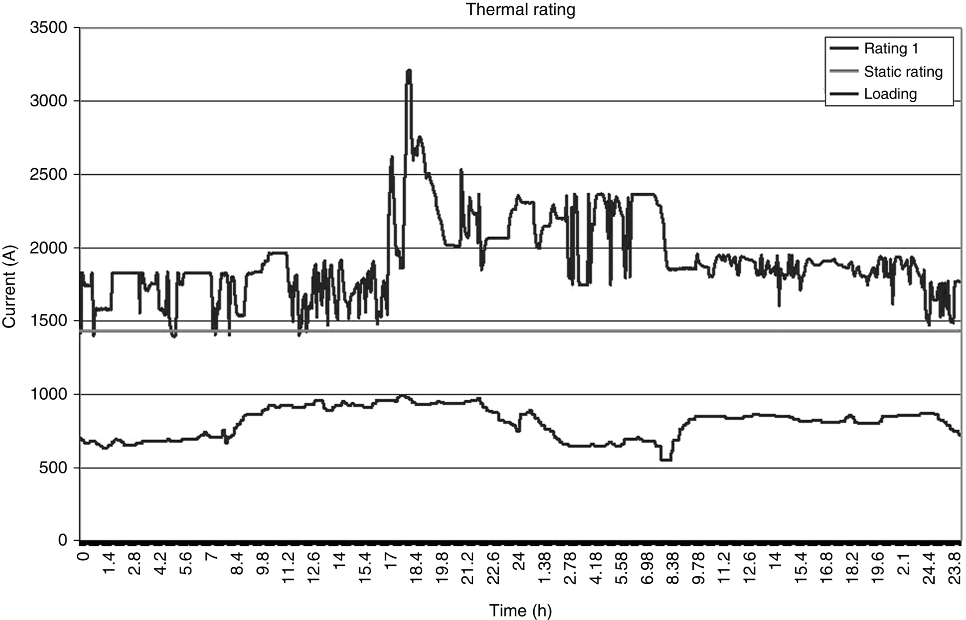
• Static rating
• Calculated dynamic rating from DTCR software
It is important to note that
• the dynamic rating is almost always greater than the static rating,
• the measured load is always significantly lower than the static rating.
For statistical representation of the thermal rating, the thermal rating data for certain duration, for example, 6 months, can be represented using probability density plot. The probability density plot shows the frequency of the thermal rating in a certain period of time. It can be used as a guide for operating the transmission line or revising the static rating. Example of the probability density plot is shown in Fig. 26.18.

The graphs show that the load is always below the static rating. Only during emergencies, the load would exceed the normal static rating. The dynamic thermal rating is mostly 20% higher than the static rating that is shown at the tip of the dynamic thermal rating probability density graph in Fig. 26.18. This is the available potential extra capacity ready to be utilized when DTCR system is used to monitor the line rating.
26.8 Overvoltages and Insulation Requirements of Transmission Lines
The considerations for insulation requirements of transmission lines are critical because overvoltages can occur as a result of lightning strokes, switching, faults, load failure, and others. Overvoltages are transitory phenomena. It is defined as any transitory voltage between phase and ground or between phases with a crest value higher than the crest value of maximum system voltage [14]. These overvoltages are often expressed in per unit values, with maximum system voltage as per unit base.
For example, the phase-to-ground per unit overvoltage is
where
Vpu=per unit phase-to-ground overvoltage
![]() =crest value of phase-to-ground overvoltage
=crest value of phase-to-ground overvoltage
Vm=maximum rms system voltage
This condition can be transient or permanent depending on its duration. Understanding overvoltage behavior including power-frequency phenomena and switching and lightning surges is important prerequisite condition in determining insulation coordination in a power system network.
The overvoltage phenomena are classified into four major classes [15]:
(a) Power-frequency overvoltages (also known as temporary overvoltages) that include Ferranti effect, self-excitation generator, overvoltage of unfaulted phases due to single-line-to-ground fault, and sudden load failure.
(b) Lower frequency harmonic resonant overvoltages that include lower order frequency resonance and local area resonant overvoltages.
(c) Switching surges that include breaker closing overvoltages, breaker tripping overvoltages, and switching surges by line switches
(d) Overvoltages by lightning strikes direct to phase conductors (direct flashover) and direct stroke to overhead shield wire or to tower structure (back flashover) or induced flashovers.
(e) Overvoltages due to abnormal conditions such as interrupted ground fault of cable, overvoltages induced on cable sheath, or touching of different kilovolts line.
In this chapter, the emphasis is given on overvoltages due to lightning strikes and switching surges and temporary overvoltages that have great impact in the selection of insulation requirements for transmission lines.
26.8.1 Overvoltage Phenomena by Lightning Strikes
By definition, lightning is an electric discharge. It is the high-current discharges of an electrostatic electricity accumulation between thundercloud and ground (cloud-to-ground discharges) or within the thundercloud (intracloud discharges). Other types of discharges such as cloud-to-cloud lightning and cloud-to-air lightning also exist but not very frequent. The thunderclouds contain ice crystals that are positively charged upper portion and water droplets that are negatively charged, usually located at lower portion of the thundercloud. The vertical circulation in terms of updrafts and downdrafts due to height and temperature effects caused disposition of charges in the thunderclouds (Fig. 26.19).
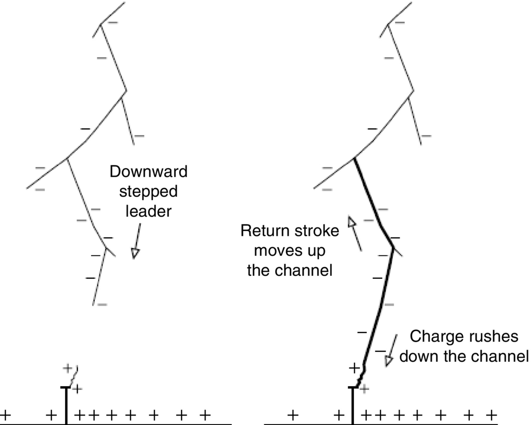
The mechanism of a lightning stroke is typically explained as follows. As the negative charges build up in the cloud base, positive charges are induced on the ground. When the voltage gradient within the cloud build up to the order of ![]() , the ionized air breaks down and creates an ionized path (leader) moving from thundercloud to ground. This initial leader progresses by series of jumps called a stepped leader. As this stepped leader (or downward leader) nears the ground, the upward leader (or return stroke) is initiated that meets the downward leader. This return stroke propagates upward from the ground to the thundercloud following the same path, at the speed of 10%–30% that of light, which is visible to the naked eye. The current involved may exceed 200 kA and lasting about 100 μs The second leader called dart leader may stroke following the same path taken by the first leader, about 40 μs later. The process of dart leader and return stroke can be repeated several times. The complete process of successive strokes are called lightning flash.
, the ionized air breaks down and creates an ionized path (leader) moving from thundercloud to ground. This initial leader progresses by series of jumps called a stepped leader. As this stepped leader (or downward leader) nears the ground, the upward leader (or return stroke) is initiated that meets the downward leader. This return stroke propagates upward from the ground to the thundercloud following the same path, at the speed of 10%–30% that of light, which is visible to the naked eye. The current involved may exceed 200 kA and lasting about 100 μs The second leader called dart leader may stroke following the same path taken by the first leader, about 40 μs later. The process of dart leader and return stroke can be repeated several times. The complete process of successive strokes are called lightning flash.
Lightning surge phenomena can be classified into three different stroke modes: (a) direct strike on phase conductors (direct flashover), (b) direct strike on shield wire or tower structure, and (c) induced strokes.
In the case of direct strike, the lightning current path is directly from the thundercloud to the line. This will cause the voltage to rise at stroke termination point, on either one phase or more phase conductors. The stroke current propagates in the form of a traveling wave in both directions and raises potential of the line to the voltage of the downward leader. Overvoltage may exceed the line-to-ground withstand voltage of line insulation and cause insulation failure, if not properly protected.
In the case of direct strike on shield wire or tower structure, a lightning stroke directly strikes the shield wire or tower structure. If lightning strikes a tower top, some of the current may flow through the shield wires, and the remaining current flows through the tower to the earth. For stroke with average current magnitude and rate of rise, the current may flow into the ground provided the tower and its footing resistance are low. Otherwise, the lightning current will raise the tower to a high voltage above the ground, causing flashover from the tower over the line insulators to one or more phase conductors.
In induced strokes, lightning strokes terminate at some point on the Earth at a short distance from a transmission line. This can be considered as a virtual wire connected to a cloud and an earth point and a surge current I(t) flowing along the virtual wire. This wire has mutual capacitances and mutual inductances across the line conductors and the shield wires of the neighborhood transmission lines. In this regard, the capacitive induced voltages and inductive induced voltage appear on the phase conductors and on the shield wires [15].
The insulation for lines is composed of air and solid dielectric insulators. The geometry of the insulators and their insulation strengths is selected to ensure that if an insulation failure occurs, the failure will be a flashover in air. This flashover produces a low-impedance path through which 50 Hz power current will flow. Generally, these arcs are not self-extinguishing. To interrupt the power fault, a protective device (circuit breaker) operating to de-energize the circuit will be required. Four types of lightning-caused flashover can occur on transmission lines: back flashover, shielding failure, induced, or midspan.
A back flashover event can occur when lightning strikes a grounded conductor or structure. In this case, a flashover proceeds backward from tower metal to the insulated conductor. A lightning stroke, terminating on an overhead ground wire or shield wire, produces waves of current and voltage that travel along the shield wire. At the tower/pole, these waves are reflected back toward the struck point and are transmitted down the tower/pole toward the ground and outward onto the adjacent shield wires. Riding along with these surge voltages are other surge voltages coupled onto the phase conductors. These waves continue to be transmitted and reflected at all points of impedance discontinuity. The surge voltages are built up at the tower/pole, across the phase-ground insulation, across the air insulation between phase conductors, and along the span across the air insulation from the shield wire to the phase conductor. If this surge voltage exceeds the insulation strength, flashover occurs. The parameters that affect the line back flashover rate (BFR) are the following:
• Surge impedances of the shield wires and tower/pole
• Coupling factors between conductors
• Power-frequency voltage
• Tower and line height
• Span length
• Insulation strength
• Footing resistance and soil composition
Sometimes, the design engineer can vary the shield wire surge impedance and the coupling factors, for example, using two shield wires instead of one. Normally, only insulation and footing impedance can be varied to improve back flashover performance. Reducing the footing impedance directly reduces the voltage stress across the insulator for a given surge current down the tower.
A shielding failure is defined as a lightning stroke that terminates on a phase conductor. For an unshielded line, all strokes to the line are shielding failures. For a transmission line with overhead shield wires, most of the lightning strokes that terminate on the line hit the shield wire and are not considered shielding failures.
The calculated number of shielding failures for a particular transmission line model depends on a number of factors, including the model's electrogeometric parameters, the stroke current distribution, and natural shielding from trees, terrain, or buildings. Not all shielding failures will result in insulator flashover. The critical current is defined as the lightning stroke current that, injected into the conductor, will result in flashover. The critical current for a particular transmission line conductor is calculated by
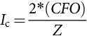
where CFO is the lightning impulse negative polarity critical flashover voltage and Z is the conductor surge impedance.
Severe transient overvoltage can be induced on overhead power lines by nearby lightning strikes. On lower voltage distribution power lines, indirect lightning strikes cause the majority of lightning-related flashovers. Estimation of indirect lightning effects is crucial for proper protection and insulation coordination of overhead lines. The problem of induced flashovers from nearby lightning strikes has received a great deal of scientific attention in the past 20 years, and the result has been the development of more accurate estimation models of lightning-induced overvoltages.
Important points to remember when dealing with induced flashovers from nearby lightning strokes include the following:
• Insulator CFO voltages above approximately 400 kV prevent nearly all induced flashovers.
• The presence of an effectively grounded overhead shield wire or neutral on the line will reduce insulator voltages by 30%–40%, depending on the line configuration.
• Line surge arresters installed every few spans can improve induced flashover performance for distribution voltage lines (spacing line arresters in this manner will seldom improve direct stroke lightning performance, only induced flashovers, and it is not recommended for transmission lines).
Power line flashovers caused by lightning strokes near midspan are unusual for most line configurations. Midspan flashovers become more likely when midspan conductor spacing is small, such as on-distribution lines, or when span lengths are very long (304.8 m or more). The voltage on a conductor follows the equation presented for a shielding failure. If the voltage rises to approximately 610 kV/m in the air gap between conductors, a long, relatively slow breakdown process might occur that might take many microseconds to complete.
26.8.2 Switching Surges
Switching surges can occur during the operation of circuit breaker and line switch opening (tripping) and closing at the same substation. In general, switching surges occur in the vicinity of non-self-restoring insulation equipment such as generators, transformers, breakers, and cables. Overvoltages caused by switching surges are a concern since they can damage insulation or cause insulation flashover. Damage and flashovers often lead to power system outage that is highly undesirable. The amplitude of a typical switching surge is about 1.5 pu with duration of about one power-frequency cycle [16].
26.8.3 Temporary Overvoltage
A temporary overvoltage is an oscillatory phase-to-ground overvoltage that is of relatively long duration and is undamped or only weakly damped. These types of overvoltages usually originate from faults, sudden changes of load, Ferranti effect, linear resonance, ferroresonance, open conductors, induced resonance from couple circuits, and others (e.g., backfeeding and stuck pole). In general, temporary overvoltage has two important characteristics: They are determinable, and they persist for many cycles. The magnitudes of these voltages may be calculated by steady-state analysis, assuming the physical conditions on the system are known.
26.9 Methods of Controlling Overvoltages
There are several means for controlling the overvoltages that occur on transmission system. Overvoltages due to switching surges can be controlled by modifying the operation of a circuit breaker or other switching device in various ways. The overvoltage may be limited to an acceptable level with the installation of surge arresters at the specific locations to be protected. The transmission system may be changed to minimize the effect of switching operations.
It is clear that if the source of the overvoltage is a random event such as lightning or fault initiation, the only sure method of controlling overvoltage will be the use of surge arresters or similar protective devices. In lightning protection design, two aspects are important to consider: (i) diversion and shielding, mainly for structural protection that also provides reduction of electric and magnetic fields within the structure, and (ii) limiting the currents and voltages on electronic, power, and communication systems through surge protection. For the latter, the protection must include the control of currents and voltages from direct strikes to the structure and from lightning-induced current and voltage surges propagating into the structure from aerial or buried conductors from outside. Four general types of current- and voltage-limiting technique are commonly used [17] which are as follows:
(a) Voltage crowbar devices such as gas-tube arresters, silicon-controlled rectifiers (SCRs), and triacs that limit overvoltages to values smaller than operating voltages and short-circuit the current to ground.
(b) Voltage clamps such as metal oxide varistors (MOVs), Zener diodes, and p-n junction transistors. These solid-state nonlinear devices reflect and absorb energy while clamping the applied voltage across terminals to 30%–50% above the system operating voltage.
(c) Circuit filters that are linear circuits that both reflect and absorb the frequencies contained in the lightning transient pulses.
(d) Isolating devices such as optical isolators and isolation transformers suppress relatively large transients.
Reduction of basic impulse insulation levels of transmission equipment is possible with the use of surge arresters. Arresters are primarily used to protect the system insulation from the effects of lightning. Nowadays, modern arresters can also control many other system surges that may be caused by switching or faults. Arresters provide indispensable aid to insulation coordination in electric power system. It has basically a nonlinear resistor so that its resistance decreases rapidly as the voltage across it rises. At the surge ends and the voltage across the arrester returns to the normal line-to-neutral voltage level, the resistance becomes high enough to limit the arc current to a value that can be quenched by the series gap of the arrester.
Surge arresters may be used to control temporary overvoltages, such as due to a fault. It may be able to protect the equipment for the short time it takes to clear the applicable breakers. Similarly, surge arresters may be used to control switching surge overvoltages along a transmission line and thus reduce the length of required insulator strings. For example, the use of metal oxide arresters at the receiving end of a 280 km line can reduce the switching overvoltage along the line from a maximum of 2.2 to 1.8 pu.
26.10 Insulation Coordination
Insulation coordination is the selection of the insulation strength [18]. The strength is selected on the basis of some quantitative or perceived degree of reliability. It is also important to know the stress placed on the insulation and methods to reduce the stress, be it through surge arresters or other means. There are three different voltage stresses to consider when determining insulation and electric clearance requirements for the design of high-voltage transmission lines: (i) the power-frequency voltage, (ii) lightning surge, and (iii) switching surge. In general, lightning surges have the highest value and the highest rates of voltage rise. Properly done insulation coordination provides assurance that the insulation used will withstand all normal discharge and a majority of abnormal discharges. Several terms used in insulation coordination are defined as follows.
The basic lightning impulse insulation level (BIL) is defined as the electric strength of insulation expressed in terms of the crest value of the “standard lightning impulse” [18]. The BILs are universally for dry conditions. It is determined by tests made using impulses of a 1.2/50-μs waveshape. Several tests are performed, and a number of flashovers are noted.
The basic lightning impulse insulation level (BSL) is the electric strength of insulation expressed in terms of the crest value of a standard switching impulse. BSLs are universally for wet conditions.
Withstand voltage is the highest voltage that the insulation can withstand without failure or disruptive discharge, under specified test conditions. It is a common practice to assign a specific testing waveshape and duration of its application to each category of overvoltage.
There are two major categories of insulation: external insulation is the distances in open air or across the surfaces of solid insulation in contact with open air that is subjected to dielectric stress and to the effects of the atmosphere. Most transmission line insulation is external insulation. Internal insulation is the internal solid, liquid, or gaseous parts of the insulation of equipment that are protected by the equipment enclosures from the effects of the atmosphere such as in a transformer.
Insulation can also be divided into self-restoring and non-self-restoring categories. Self-restoring insulation completely recovers its insulating properties after a disruptive discharge. Non-self-restoring insulation loses insulation properties or does not recover completely after a disruptive discharge. Most external insulation, such as external air gap, is self-restoring insulation, and most internal insulation, such as solid insulation in a transformer, is non-self-restoring insulation. Insulation failure consequences are different for the different categories. Failure of non-self-restoring internal insulation is catastrophic, while failure of external self-restoring insulation may only be a nuisance. Testing may be done after a disruptive discharge for self-restoring internal insulation that provides statistical data for examination.
Insulation coordination involves the following processes: (i) determination of line insulation, (ii) selection of BIL and insulation levels of other equipment, and (iii) selection of lightning arresters. To assist this process, standard insulation levels are recommended such as in IEC Publication 71.1 “Insulation Coordination Part 1, Definitions, Principles and Rules,” 1993–12.
Knowledge of the overvoltages that the system will be exposed may be gained in two general ways: by measurement on the real system or by analysis on related models. Field measurement on a real system can only be done after the system is built. Analytic method can be used to determine the magnitude of overvoltages. The transient behavior of a complex transmission system must be studied through models either analog or digital. Transient network analyzer is an example on an analog model. For transmission lines below 345 kV, the line insulation is determined by lightning flashover rate. At 345 kV, the line insulation may be dictated either by switching surge or by lightning flashover rate. Above 345 kV, switching surges become a major factor in flashover considerations. The probability of flashover due to a switching surge is a function of the line characteristics and the magnitude of the surges expected. The number of insulators may be selected to keep the probability of flashovers due to switching surge very low.
In the design of substation, the maximum switching surge level used is either the maximum surge that can take place in the system or the protective level of arresters. In this case, the insulation coordination in a substation involves the selection of the minimum arrester rating applicable to withstand the power-frequency voltage and the equipment insulation level to be protected by arresters.