
Fuzzy-Logic Applications in Electric Drives and Power Electronics
Abdul R. Ofoli The University of Tennessee at Chattanooga, Chattanooga, TN, United States
Abstract
The use of an extended Kalman filter to train fuzzy neural network structures for online speed trajectory tracking of a brushless drive system is illustrated as an alternative to control schemes. Also described in this chapter is an implementation of a genetic-based hybrid fuzzy-proportional-integral-derivative (PID) controller for industrial motor drives. The genetic optimization technique is used to determine the optimal values of the scaling factors of the output variables of the fuzzy-PID (FPID) controller. The objective is to utilize the best attributes of the PID and FPID controllers to produce better response under disturbance. In servomotor drive tracking applications where we need to compensate for system uncertainty and random changes, a control structure that employs a fuzzy-logic controller incorporating an H-infinity tracking controller via an acceleration feedback signal is explained. The chapter ends with the implementation of a fuzzy-logic controller structure for switch-mode power-stage DC-DC converters and evaluates experimentally its sensitivity for variable supply voltages and load resistance variations.
Keywords
Extended Kalman filter (EKF); Fuzzy neural network (FNN); Motor drives; Proportional-integral-derivative (PID) controllers; dSPACE digital signal processor (DSP); Genetic optimization; Hybrid fuzzy-PID controller; Brushless servo drives; Fuzzy-logic controller; H-infinity controller; DC-DC converter; Learning algorithm; Real-time implementation
Acknowledgments
We will like to acknowledge Dr. Ahmed Rubaai at Howard University, Dr. Paul Young of RadiantBlue Technologies and Dr. Marcel J. Castro-Sitiriche at the Electrical and Computer Engineering Department, of the University of Puerto Rico at Mayagüez, for their contribution to the third edition of this chapter.
36.1 Introduction
Improving the popular proportional-integral-derivative (PID) controller using fuzzy logic (FL) is currently an important research topic. Years of various applications have shown different techniques for customizing the PID controller [1–7]. Recent work by Sant [1] employs an FL controller combined with a classical PID controller with a switching function between them for speed control of a motor drive. The switching algorithm allows each controller type to perform better under different operations. In another recent example, Hohan [2] has developed a fuzzy-PID controller based upon the error, the difference in error, and the difference to create a delta change in the control signal at each time step. Hohan includes analytic stability analysis for bounded inputs, important for fuzzy systems to gain acceptance among control engineers. The application of fuzzy reasoning to improve the PID controller is evident in the research community today to build state-of-the-art control systems. Recent work on self-tuning PID controllers demonstrates adaptive control of motor drive systems. Typically, an engineer might retune the gains of a nominal PID controller during operation, but an adaptive PID system autonomously tunes gains as performance diminishes. The work of Rubaai [3] employs a genetic algorithm to evolve optimal scale factors of fuzzy-based PID gains for improved control of a motor drive. This genetic-based scale factor in conjunction with FL gain selection enhances the sensitivity of the PID control to error. Another class of fuzzy-PID control design mimics PID control via blending FL networks with absolute and incremental control values at a given control time step. The work of Kuo [4] employs two FL structures to formulate a control of a suspension system. One FL mimics PD control, while the other FL generates a change in control to mimic a PI control signal. These FL structures adapt using a genetic algorithm as well. The work of Hu [5] also employs fuzzy-PD and fuzzy-PI elements as part of a control strategy. Li [6] designs an FL based on error and error derivative to generate an initial control estimate that then feeds a PI logic and a PD logic. This work demonstrates robustness of the control algorithm through simulations of a dynamic model. The recent work of Masiala [7] demonstrates incremental fuzzy-PI control of an induction motor drive. For Masiala, the FL decision at each time step modifies the control current based on the error and a change in error. All these controllers use FL to generate absolute and incremental control signals to mimic control techniques seen in PID control. Kalman filter (KF) is another research topic that has been applied to a wide range of engineering disciplines. For a linear system, the KF is an established control design feature, but the improved application of variants of the KF to account for nonlinearity in systems inspires research today. Barut [8] employs an extended Kalman filter (EKF) for a speed sensorless control of an induction motor. This work depends on high-fidelity equations of motion model and noise characteristics. Szabat [9] demonstrates an adaptively tuned EKF for control of an industrial drive. Ahn [10] designs an EKF algorithm to update parameters of parallel FL systems, which generate a PID gain set for control of a motor drive system. Treating the controller as a process and deriving appropriate derivatives allow for adaptive update to the FL components. So, while PID control is a commonly known algorithm, current research applications of adaptive tuning are yielding better tuned PID systems. The artificial neural network (ANN) is a computational data structure modeled after the firing of neurons in the brain. Training exercises may adjust the parameters within the ANN to improve modeling capabilities. The work of Lary [11] details an EKF algorithm for training an ANN to model correlations between chemical compounds. Singhal [12] shows that the EKF training algorithm treats all ANN parameters as a state vector, and thus, the ANN becomes a nonlinear stationary process. Research experience demonstrates that the EKF training compares favorably to the BP update method in terms of iterations of training epochs, but with higher computational cost per time step. The ANN is an important contribution to the control field. The fuzzy neural network (FNN) combines aspects of FL and the ANN and is at the state of the art in control research today. For example, recent work of Ho [13] simulates PID control using an FNN structure that updates time constants in the dynamic models that generate the PID gains online. Ho compares the orthogonal simulated annealing learning technique to a genetic technique to improve performance of the FNN portion of the controller. Campo [14] designs an embedded hardware FNN updated by the Takagi-Sugeno training method for performance improvement. Such a chip enables for a fuzzy system embedded into a hardware control loop. Uddin [15] also developed a hybrid neuro-fuzzy-PI controller adapted by a real-coded genetic algorithm to control an IPMSM. In this case, a fuzzy basis function network similar to an FNN output PI gains sensitive to error conditions. The cutting-edge work of many researchers today relies on the FNN to improve the performance of fuzzy control systems in electric applications.
36.2 PI/PD-Like Fuzzy Control Structure
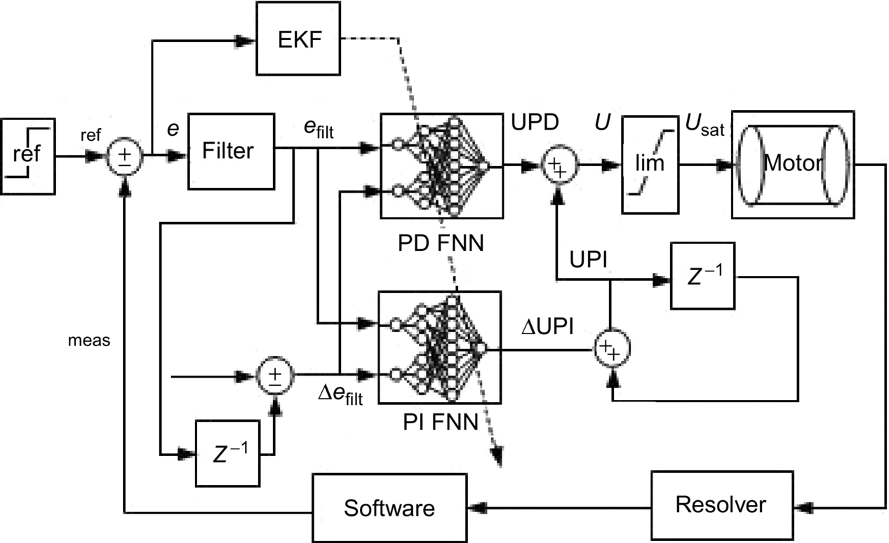
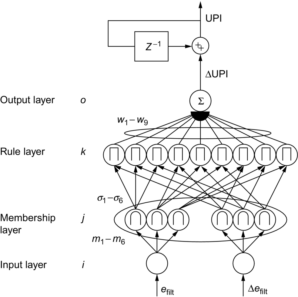
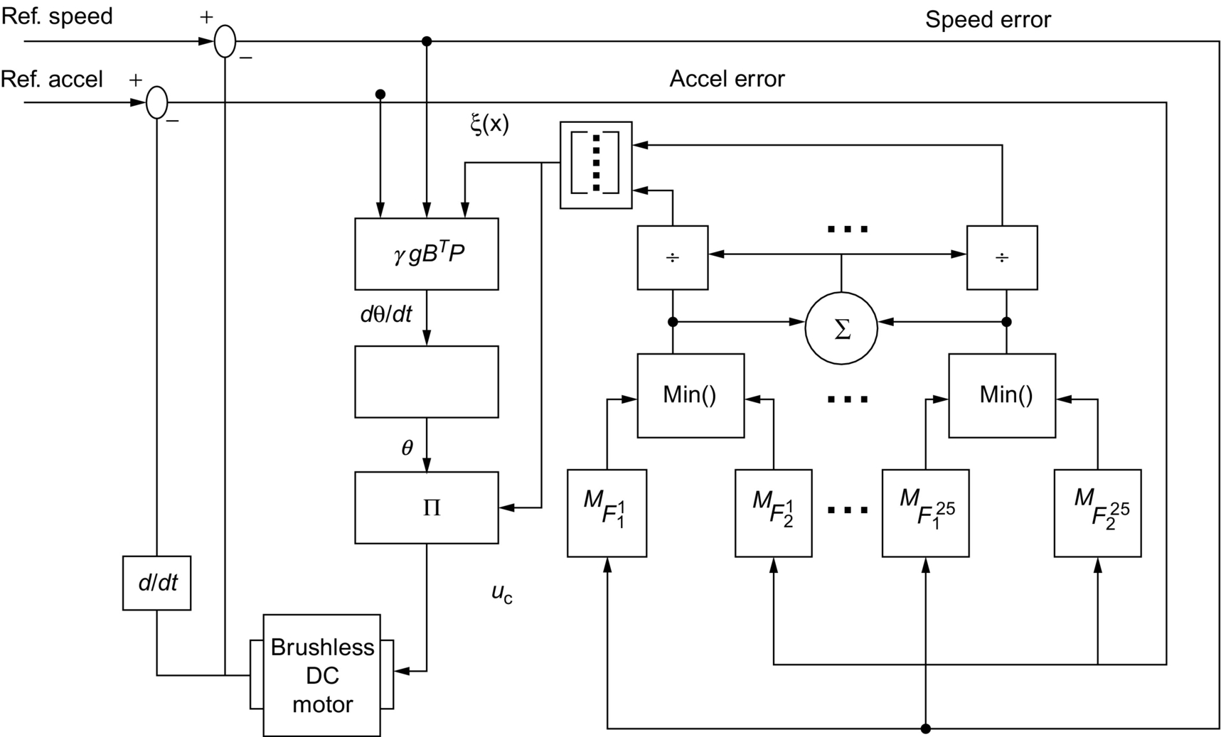
The FNN PI/PD-like fuzzy controller using EKF control structure presented in this chapter is an instantiation of a feedback control loop. The FNN PI/PD-like fuzzy consists of two independent fuzzy structures, namely, fuzzy-PD controller and fuzzy-PI controller. EKF technique is used to modify the weights and the membership functions of the FNN PI/PD controller to adaptively control the rotor speed of the drive system. The summation of the outputs of the two FNNs forms the control signal. Fig. 36.1 shows the architecture of the neural-fuzzy PI-/PD-based EKF learning scheme. The control structure is anticipated to accommodate the robust stabilization and disturbance rejection problems. The fuzzy controller generates a control signal based upon two FL structures. The first structure is a fuzzy PD that generates a fuzzy-PD control signal. The second structure is a fuzzy PI that generates an incremental fuzzy-PI control signal.
UPD=FLPD(efilt,Δefilt)
ΔUPI=FLPI(efilt,Δefilt)
The incremental fuzzy-PI signal sums with the previous fuzzy-PI signal to generate the fuzzy-PI signal for the time step at hand. The fuzzy-PI/fuzzy-PD controller generates a control signal with the summation of the fuzzy-PI/fuzzy-PD control signals:
U=UPD+UPI
The control signal is limited by a discontinuous range-limiting saturation element. The saturation equation caps the signal between a maximum and minimum value:
usat=umaxifU>umaxuminifU<uminUotherwise

36.2.1 Fuzzy-Based PI Controller
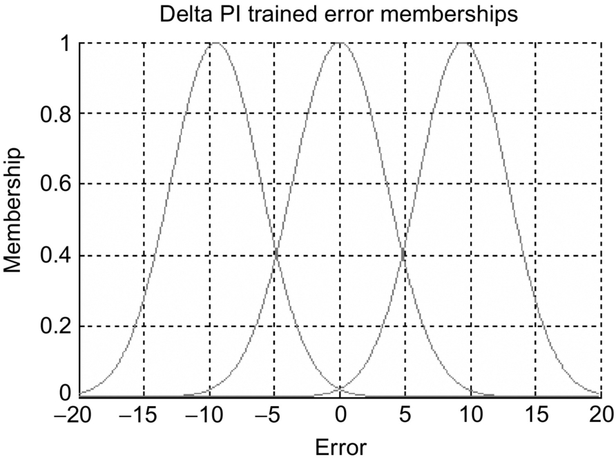
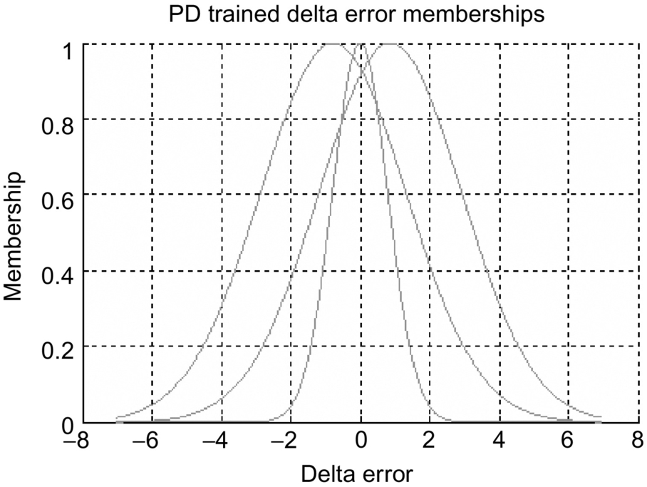
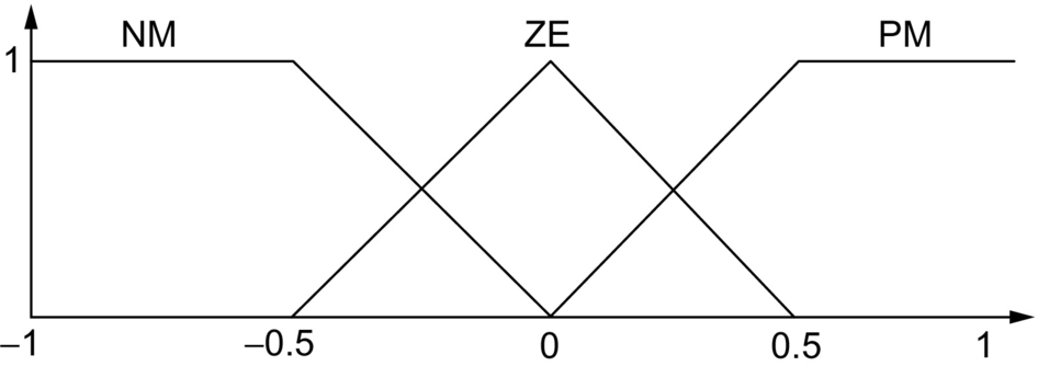
The fuzzy-PI system implements an FL for the PI control signals efilt and Δefilt, the error and the delta error, respectively, the linguistic inputs to the system. The FL output is the PI control ΔUPI signal. The error signal has three fuzzy variables: positive (P), zero (Z), and negative (N). The delta error signal has three fuzzy variables: positive (P), zero (Z), and negative (N). The membership function for each fuzzy variable is a Gaussian function. Figs. 36.2 and 36.3 display the trained membership functions for the fuzzy inputs.

The linguistic control rules are established considering the dynamic behavior of the BLDC drive system and analyzing the error and its variation. The fuzzy inference system has nine rules.
Rule 1: IF speed error is negative (N) AND delta speed error is negative (N), THEN the fuzzy-PI control voltage (output of FL) is negative large (NL). This rule pertains to the condition that wref<wmeas![]() and that the difference between them is increasing. Thus, the control action must act to change the error momentum and bring the motor rate back down to the reference rate. Therefore, a large negative change in control voltage is necessary.
and that the difference between them is increasing. Thus, the control action must act to change the error momentum and bring the motor rate back down to the reference rate. Therefore, a large negative change in control voltage is necessary.
Rule 2: IF speed error is negative (N) AND delta speed error is zero (Z), THEN the fuzzy-PI control voltage (output of FL) is negative medium (NM). This rule pertains to the condition that wref<wmeas![]() and that the difference between them is steady. Thus, the control action need not change the error momentum but still bring the motor rate back down to the reference rate. Therefore, a medium negative change in control voltage is necessary.
and that the difference between them is steady. Thus, the control action need not change the error momentum but still bring the motor rate back down to the reference rate. Therefore, a medium negative change in control voltage is necessary.
Rule 3: IF speed error is zero (Z) AND delta speed error is negative (N), THEN the fuzzy-PI control voltage (output of FL) is negative small (NS). This rule pertains to the condition that wref=wmeas![]() but tending toward wref<wmeas
but tending toward wref<wmeas![]() as the error trends more negative. Thus, the control action must act to halt the error momentum but maintain the motor rate being close to the reference rate. Therefore, a small negative change in control voltage is necessary.
as the error trends more negative. Thus, the control action must act to halt the error momentum but maintain the motor rate being close to the reference rate. Therefore, a small negative change in control voltage is necessary.
Rule 4: IF speed error is negative (N) AND delta speed error is positive (P), THEN the fuzzy-PI control voltage (output of FL) is zero (ZE). This rule pertains to the condition that wref<wmeas![]() and that the difference between them is decreasing. Thus, the control action of nothing allows the error momentum to bring the motor rate back down to the reference rate. Therefore, no change in control voltage is necessary.
and that the difference between them is decreasing. Thus, the control action of nothing allows the error momentum to bring the motor rate back down to the reference rate. Therefore, no change in control voltage is necessary.
Rule 5: IF speed error is zero (Z) AND delta speed error is zero (Z), THEN the fuzzy-PI control voltage (output of FL) is zero (ZE). This rule pertains to the condition that wref=wmeas![]() and that the difference between them is steady. Thus, the control action of nothing allows the error momentum to remain negligible to leave the motor rate at the reference rate. Therefore, no change in control voltage is necessary.
and that the difference between them is steady. Thus, the control action of nothing allows the error momentum to remain negligible to leave the motor rate at the reference rate. Therefore, no change in control voltage is necessary.
Rule 6: IF speed error is positive (P) AND delta speed error is positive (P), THEN the fuzzy-PI control voltage (output of FL) is positive large (PL). This rule pertains to the condition that wref>wmeas![]() and that the difference between them is increasing. Thus, the control action must act to change the error momentum and bring the motor rate back up to the reference rate. Therefore, a large positive change in control voltage is necessary.
and that the difference between them is increasing. Thus, the control action must act to change the error momentum and bring the motor rate back up to the reference rate. Therefore, a large positive change in control voltage is necessary.
Rule 7: IF speed error is positive (P) AND delta speed error is zero (Z), THEN the fuzzy-PI control voltage (output of FL) is negative medium (NM). This rule pertains to the condition that wref>wmeas![]() and that the difference between them is steady. Thus, the control action need not change the error momentum but still bring the motor rate back down to the reference rate. Therefore, a medium positive change in control voltage is necessary.
and that the difference between them is steady. Thus, the control action need not change the error momentum but still bring the motor rate back down to the reference rate. Therefore, a medium positive change in control voltage is necessary.
Rule 8: IF speed error is zero (Z) AND delta speed error is positive (P), THEN the fuzzy-PI control voltage (output of FL) is positive small (PS). This rule pertains to the condition that wref=wmeas![]() but tending toward wref>wmeas
but tending toward wref>wmeas![]() as the error trends more positive. Thus, the control action must act to halt the error momentum but maintain the motor rate being close to the reference rate. Therefore, a small positive change in control voltage is necessary.
as the error trends more positive. Thus, the control action must act to halt the error momentum but maintain the motor rate being close to the reference rate. Therefore, a small positive change in control voltage is necessary.
Rule 9: IF speed error is positive (P) AND delta speed error is negative (N), THEN the fuzzy-PI control voltage (output of FL) is zero (ZE). This rule pertains to the condition that wref>wmeas![]() and that the difference between them is decreasing. Thus, the control action of nothing allows the error momentum to bring the motor rate back down to the reference rate. Therefore, no change in control voltage is necessary.
and that the difference between them is decreasing. Thus, the control action of nothing allows the error momentum to bring the motor rate back down to the reference rate. Therefore, no change in control voltage is necessary.
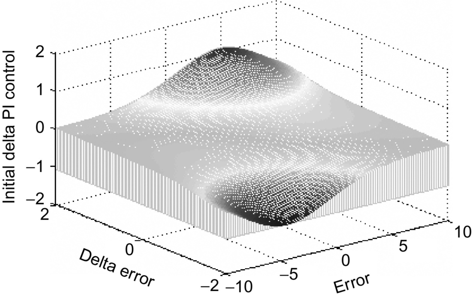
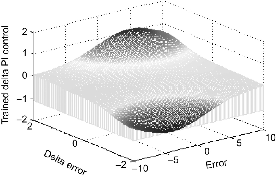
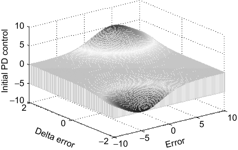
Each rule is implemented via a weighted product of the membership variables. The fuzzy centroid method generates a crisp output from the nine-dimensional fuzzy rule vector. This scaled output corresponds to the control signal, ΔUPI. Figs. 36.4 and 36.5 illustrate the initial and trained fuzzy control output ΔUPI as a function of the error and the change of error.
36.2.2 Fuzzy-Based PD Controller
The same technique applied to the fuzzy-PI controller is applied to the fuzzy-PD controller. The controller has two inputs and one output. The fuzzy-PD system implements an FL for the PD control signal. The signals efilt and Δefilt, the error and the delta error, respectively, are the linguistic inputs to the system. The FL output is the PD control signal UPD. The error signal has three fuzzy variables: positive (P), zero (Z), and negative (N). The delta error signal has three fuzzy variables: positive (P), zero (Z), and negative (N). The membership function for each fuzzy variable is a Gaussian function. Figs. 36.6 and 36.7 show the trained membership functions for the PD fuzzy inputs.

Similarly, the number of fuzzy rules that are required is equal to the product of the number of fuzzy sets that make up each of the two fuzzy input variables. Therefore, a total of nine fuzzy rules are instituted. The nine fuzzy rules are composed of the same fuzzy rules generated for the fuzzy-PI controller and are not repeated here. Each rule is implemented via a weighted product of the membership variables. The fuzzy centroid method generates a crisp output from the nine-dimensional fuzzy rule vector. This scaled output corresponds to the control signal, UPD. Figs. 36.8 and 36.9 demonstrate the initial and trained fuzzy control output, UPD, as a function of the error and the change of error.
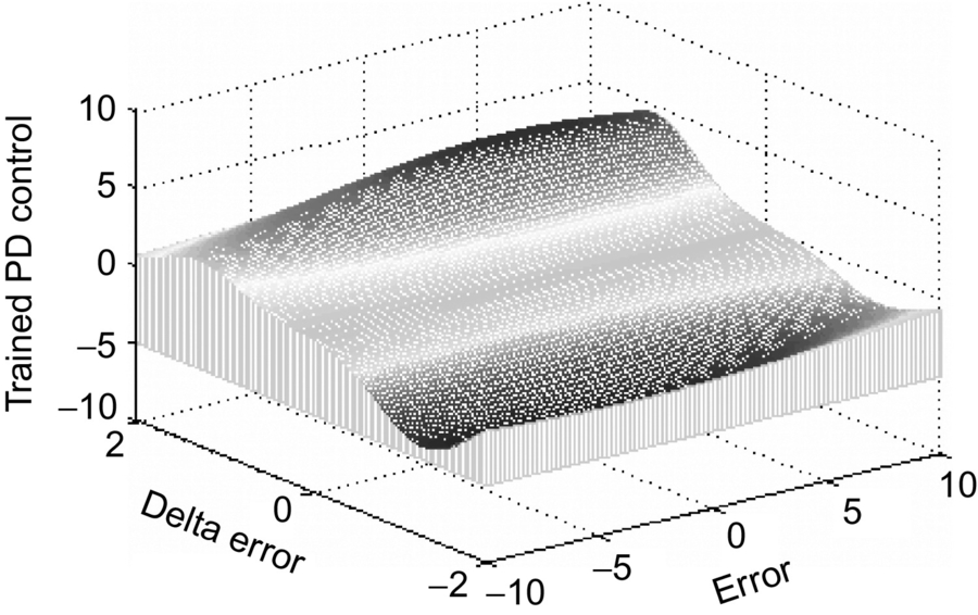
Figs. 36.8 and 36.9 provide an indication of how well the EKF learning algorithm succeeds in training the output fuzzy-PD control signal. This is an indication of how well the control process is proceeding during the experimental implementation.
36.3 FNN PI/PD-Like Fuzzy Control Architecture
The proposed FNN has four layers: an input layer, a membership layer, a rule layer, and an output layer. The input layer is a pass-through capture of each input signal. The membership layer creates a fuzzy set for each input using Gaussian membership functions. The rule layer consists of a truth table like evaluation of the fuzzy membership sets by product pairing. The output layer consists of a weighted summation of the rules. Three numbers define the size of an FNN: the number of inputs to the logic, the number of memberships per input, and the number of outputs, respectively, that is, 2×3×1![]() . The PI/PD demands two 2×M×1
. The PI/PD demands two 2×M×1![]() FNNs, where M, the number of memberships, is customizable. A larger number of memberships enhance accuracy of the FNN for modeling; however, a smaller number of memberships yields a smaller training calculation time period per step (there are less calculations to perform) enabling a faster system rate on real-time hardware. The membership number of 3 is selected. The parameters of the FNN are the means and sigmas of the Gaussian memberships and the weights of the output layer. For a 2×3×1
FNNs, where M, the number of memberships, is customizable. A larger number of memberships enhance accuracy of the FNN for modeling; however, a smaller number of memberships yields a smaller training calculation time period per step (there are less calculations to perform) enabling a faster system rate on real-time hardware. The membership number of 3 is selected. The parameters of the FNN are the means and sigmas of the Gaussian memberships and the weights of the output layer. For a 2×3×1![]() FNN, there are (six means + six sigmas + nine weights) 21 parameters. Figs. 36.10 and 36.11 display the structure of FNN-based PI and FNN-based PD. Below is the definition of the function of each layer.
FNN, there are (six means + six sigmas + nine weights) 21 parameters. Figs. 36.10 and 36.11 display the structure of FNN-based PI and FNN-based PD. Below is the definition of the function of each layer.
 FNN PI structure.
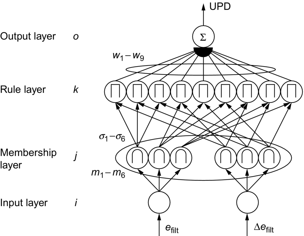 FNN PD structure.
36.3.1 Input Layer
The input layer passes the input value, assigned for each FNN as follows (let be the feedback error).

36.3.2 The Membership Layer
Each membership function into the fuzzy set is a Gaussian; the following evaluation occurs (note that mij and σij are parameters):
ymemij=exp(ui−mij)2σ2ij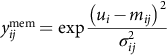 for input i=1,2
![]() and member j=1,2,3
and member j=1,2,3![]() of that input.
of that input.
For further derivations, allow the matrix ymem to be vectorized as follows:
ymem1=ymem11,ymem2=ymem12,ymem3=ymem13,ymem4=ymem21,ymem5=ymem22,ymem6=ymem23

and allow the same vectorization for the means m matrix into a vector and sigmas σ matrix into a vector.
36.3.3 The Rule Layer
Each rule function is a product of two membership outputs. Refer to the table: each table cell is a rule layer output calculated by the product of the row and column label values.
36.3.4 The Output Layer
The weighted summation of the rules composes the output layer (note parameters Wk): y=Σ9k=1yrulekWk![]() where k=1,9
where k=1,9![]() .
.
36.4 Learning Algorithm-Based EKF
At each time step, for each 2×3×1![]() FNN, there is a state vector comprised of 21 elements: x=[W1⋯W9,m1⋯m6,σ1⋯σ6]
FNN, there is a state vector comprised of 21 elements: x=[W1⋯W9,m1⋯m6,σ1⋯σ6]![]() (noting vector form of m,σ).
(noting vector form of m,σ).
Furthermore, define the following: the reference model output ωref, measured output ωmeas, control signal U, PI FNN output control signal ΔUPI, and PD FNN output control signal UPD. Also, allow for the matrix notation of the membership outputs to be vectorized as follows:
The EKF innovation process is the difference from a reference signal to the measured output of the system ˜Z=ωref−ωmeas![]() . A state gradient vector h must be created, such that hi=d(ωmeas)/dxi
. A state gradient vector h must be created, such that hi=d(ωmeas)/dxi![]() using the chain rule backpropagation. The change in system output with respect to input (ωmeas)/d(U) is assumed as unity. This is a dangerous assumption, and a more sophisticated control algorithm would attempt to model this scalar value, perhaps with an FNN identification structure.
using the chain rule backpropagation. The change in system output with respect to input (ωmeas)/d(U) is assumed as unity. This is a dangerous assumption, and a more sophisticated control algorithm would attempt to model this scalar value, perhaps with an FNN identification structure.
The control signal is the summation U=UPI+UPD![]() . Thus, to propagate into each FNN, the following are useful: d(U)/d(UPI)=1
. Thus, to propagate into each FNN, the following are useful: d(U)/d(UPI)=1![]() and d(U)/d(UPD)=1
and d(U)/d(UPD)=1![]() and d(UPI)/d(ΔUPI)=1
and d(UPI)/d(ΔUPI)=1![]() .
.
Within the FNN, the change in output layer calculation with respect to each weight is d(y)/d(Wk)=yrulek![]() for k=[1,9]
for k=[1,9]![]() and note y=ΔUPI
and note y=ΔUPI![]() and y=UPD
and y=UPD![]() for each FNN.
for each FNN.
Within the FNN, to propagate to the membership layer, the vector d(y)/d(yrulek)=Wk![]() is the change in the FNN output with respect to each rule.
is the change in the FNN output with respect to each rule.
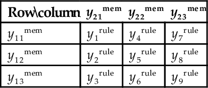
Each rule is a product of two fuzzy set elements from the membership layer. The following matrix defines the gradient of rules to a vector form of membership outputs.
d(yrule)Td(ymem)=[ymem400ymem!00ymem5000ymem10ymem60000ymem10ymem40ymem2000ymem500ymem200ymem6000ymem200ymem4ymem30000ymem50ymem3000ymem600ymem3]
Each membership is Gaussian. The partial with respect to the mean and sigma are necessary:
d(ymemij)/d(mij)=ymemij2(ui−mij)/σ2ij
and
d(ymemij)/d(σij)=ymemij2(ui−mij)2/σ3ij
Note that the resulting matrix may be vectorized as seen previously for ymem.
Applying the chain rule, the following gradients for each FNN are (where y=ΔUPI![]() and y=UPD
and y=UPD![]() for each respective calculation) and ∗
for each respective calculation) and ∗![]() represents element-wise multiplication:
represents element-wise multiplication:
d(ωmeas)/d(w)=d(ωmeas)d(U)d(U)d(y)d(y)d(W)d(ωmeas)/d(m)=d(ωmeas)d(U)d(U)d(y)d(y)Td(yrule)d(yrule)TTd(ymem)∗d(ymem)d(m)d(ωmeas)/d(σ)=d(ωmeas)d(U)d(U)d(y)d(y)Td(yrule)d(yrule)TTd(ymem)∗d(ymem)d(σ)
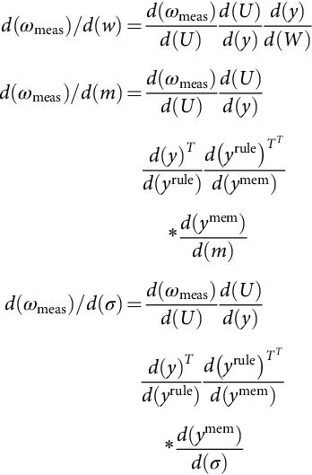
The gradient state vector is then a concatenation:
h=[d(ωmeas)d(w)λw,d(ωmeas)d(m)λm,d(ωmeas)d(σ)λσ]
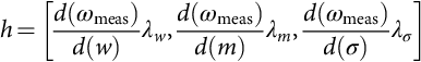
where λw,λm, and λσ are learning rate constants for the weights, means, and sigmas.
The EKF algorithm consists of the following recursive equations built on the state vector x and gradient state vector h (both 21×1![]() below) and a state covariance matrix P and measurement noise scalar r and state noise vector q:
below) and a state covariance matrix P and measurement noise scalar r and state noise vector q:
k=(Ph)/(r+hTPh)xnext=x+k˜zPnext=P−khTP+q

36.5 Fuzzy PID Control Design-Based Genetic Optimization
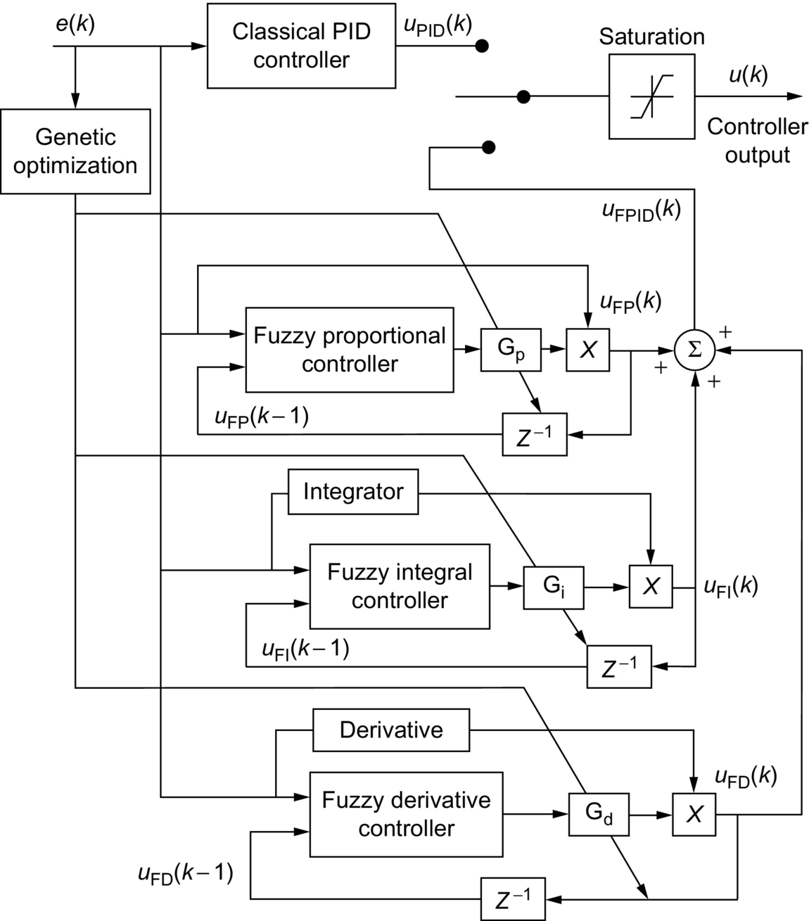
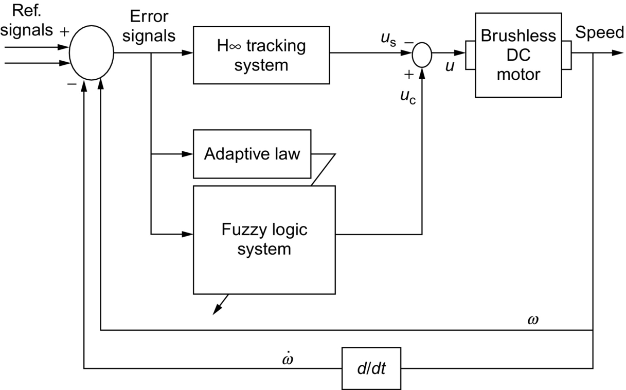
A genetic-based hybrid fuzzy-PID controller, which employs a fuzzy-PID controller integrating a classical PID controller, is presented in this section. The fuzzy-PID controller consists of three parallel fuzzy subcontrollers, namely, fuzzy-based proportional controller, fuzzy-based integral controller, and fuzzy-based derivative controller. A genetic optimization technique is used to determine the optimal values of the scaling factors of the output variables of these subcontrollers. These independent controllers are grouped together and integrated with an industrial PID controller to form a hybrid fuzzy-PID controller. Fig. 36.12 shows the architecture of the proposed genetic-based hybrid fuzzy-PID controller. The hybrid fuzzy-PID controller is anticipated to accommodate the robust stabilization and disturbance rejection problems.
36.5.1 Fuzzy-Based Proportional Controller
The first step in designing the controller is to decide which state variables of the drive system can be taken as the input signals to the controller. Both the speed error, e(k), and the delayed feedback control signal, uFP(k−1)![]() , are used as the inputs to the speed controller. The output of the fuzzy-based proportional controllers is the gain, FKP. The linguistic fuzzy variable “e(k)” has three sets: positive large (PL), zero (ZE), and negative large (NL), with each set having its own membership function. Furthermore, the linguistic fuzzy variable “uFP(k−1)
, are used as the inputs to the speed controller. The output of the fuzzy-based proportional controllers is the gain, FKP. The linguistic fuzzy variable “e(k)” has three sets: positive large (PL), zero (ZE), and negative large (NL), with each set having its own membership function. Furthermore, the linguistic fuzzy variable “uFP(k−1)![]() ” also has three sets: positive large (PL), zero (ZE), and negative large (NL), with each set having its own membership function. After specifying the fuzzy sets, it is required to determine the membership functions for these sets. Typical triangular membership functions are utilized for the e(k) and uFP(k−1)
” also has three sets: positive large (PL), zero (ZE), and negative large (NL), with each set having its own membership function. After specifying the fuzzy sets, it is required to determine the membership functions for these sets. Typical triangular membership functions are utilized for the e(k) and uFP(k−1)![]() . The three fuzzy sets can be symbolized by Fji,i=1,2
. The three fuzzy sets can be symbolized by Fji,i=1,2![]() and j=1,2,3.
and j=1,2,3.![]() Their corresponding membership functions can be symbolized by μFj(e,uFP(k−1)),j=1,2,3
Their corresponding membership functions can be symbolized by μFj(e,uFP(k−1)),j=1,2,3![]() .
.
The next step in the design of the fuzzy subcontroller is the determination of the fuzzy IF-THEN inference rules. The number of fuzzy rules that are required is equal to the product of the number of fuzzy sets that make up each of the two fuzzy input variables. Thus, a total of nine fuzzy rules are required to relate each possible combination of the two fuzzy input variables to the output membership fuzzy sets. The fuzzy rules ensure that the output of each fuzzy controller enhances the overall speed-tracking performance. Examples of such rules are the following:
IF e(k) is positive large AND uFP(k−1)![]() is negative large, THEN FKP is positive medium (PM).
is negative large, THEN FKP is positive medium (PM).
IF e(k) is zero AND uFP(k−1)![]() is zero, THEN FKP is positive small (PS).
is zero, THEN FKP is positive small (PS).
IF e(k) is positive large AND uFP(k−1)![]() is zero, THEN FKP is positive very large (PVL).
is zero, THEN FKP is positive very large (PVL).
In general, a typical fuzzy rule is of the form:
R(k): IF e(k) is F1j, and uFP(k−1)![]() is F2l, THEN fP is Ckl for j=1…3,l=1…3,k=1…9
is F2l, THEN fP is Ckl for j=1…3,l=1…3,k=1…9![]() .
.
The conjunction of the rule antecedents is evaluated by the fuzzy operation intersection, which is implemented by the min operator. The rule strength represents the degree of membership of the output variable for a particular rule. Defining the rule strength, ξi,j of a particular rule as ξi,j=min(μFi,μFj)![]() where i∈[PL,ZE,NL]
where i∈[PL,ZE,NL]![]() is associated with the fuzzy variable, e(k), and j∈[PL,ZE,NL]
is associated with the fuzzy variable, e(k), and j∈[PL,ZE,NL]![]() is associated with the fuzzy variable, uFP(k−1)
is associated with the fuzzy variable, uFP(k−1)![]() . The fuzzy inference engine uses the appropriately designed knowledge base to evaluate the fuzzy rules and produce an output for each rule. Subsequently, the multiple outputs are transformed to a crisp output by the defuzzification interface. Once the aggregated fuzzy set representing the fuzzy output variable has been determined, an actual crisp control decision must be made. The process of decoding the output to produce an actual value for the controller gain FKP is referred to as defuzzification. Thus, a fuzzy-logic controller-based center-average defuzzifier is implemented. The output of fuzzy-based proportional controller is given by FKP=fP(e(k),uFP(k−1))
. The fuzzy inference engine uses the appropriately designed knowledge base to evaluate the fuzzy rules and produce an output for each rule. Subsequently, the multiple outputs are transformed to a crisp output by the defuzzification interface. Once the aggregated fuzzy set representing the fuzzy output variable has been determined, an actual crisp control decision must be made. The process of decoding the output to produce an actual value for the controller gain FKP is referred to as defuzzification. Thus, a fuzzy-logic controller-based center-average defuzzifier is implemented. The output of fuzzy-based proportional controller is given by FKP=fP(e(k),uFP(k−1))![]() , where
, where
fP(e(k),uFP(k−1))=9∑1=1μOl(mini=1,2(μFli(e(k),uFP(k−1))))9∑l=1(mini=1,2(μFli(e(k),uFP(k−1))))

The linguistic fuzzy output variable “FKP” has nine sets: negative very large (NVL), negative large (NL), negative medium (NM), and negative small (NS), zero (ZE), positive small (PS), positive medium (PM), positive large (PL), and positive very large (PVL). The two fuzzy sets, namely, negative very large (NVL) and positive very large (PVL), are added to enhance the tracking performance. After specifying the fuzzy sets, it is required to determine the membership functions for these sets μOl for l=1…9![]() . The membership function for the fuzzy set-representing zero is a fuzzy singleton. Additionally, the other membership functions are composed of fuzzy singletons within the region defined for the fuzzy output variable. Consequently, the control signal generated by the fuzzy-proportional controller can be written as uFP(k)=GP{fP(e(k),uFP(k−1))}e(k)
. The membership function for the fuzzy set-representing zero is a fuzzy singleton. Additionally, the other membership functions are composed of fuzzy singletons within the region defined for the fuzzy output variable. Consequently, the control signal generated by the fuzzy-proportional controller can be written as uFP(k)=GP{fP(e(k),uFP(k−1))}e(k)![]() , where GP is the scaling factor that is tuned experimentally using genetic optimization.
, where GP is the scaling factor that is tuned experimentally using genetic optimization.
36.5.2 Fuzzy-Based Integral Controller
The same technique applied to the fuzzy-based proportional controller is applied to the fuzzy-based integral controller. The controller has two inputs and one output. The inputs to the fuzzy-based controller are (1) the angular speed error, e(k), and (2) the delayed feedback control signal, uFI(k−1)![]() . The controller output is the gain, FKI, of the controller. Three fuzzy sets are defined for the fuzzy linguistic variable “e(k)” and three fuzzy sets for the fuzzy linguistic variable “uFI(k−1).”
. The controller output is the gain, FKI, of the controller. Three fuzzy sets are defined for the fuzzy linguistic variable “e(k)” and three fuzzy sets for the fuzzy linguistic variable “uFI(k−1).”![]() After specifying the fuzzy sets of the two fuzzy variables, the membership functions for these sets are derived. The membership functions are composed of the same fuzzy triangular membership functions allocated for the fuzzy-based proportional controller. Similarly, the number of fuzzy rules that are required is equal to the product of the number of fuzzy sets that make up each of the two fuzzy input variables. Therefore, a total of nine fuzzy rules are introduced. Some of these rules and their significance are explained as follows:
After specifying the fuzzy sets of the two fuzzy variables, the membership functions for these sets are derived. The membership functions are composed of the same fuzzy triangular membership functions allocated for the fuzzy-based proportional controller. Similarly, the number of fuzzy rules that are required is equal to the product of the number of fuzzy sets that make up each of the two fuzzy input variables. Therefore, a total of nine fuzzy rules are introduced. Some of these rules and their significance are explained as follows:
Rule 1: IF e(k) is positive large (PL) AND uFI(k−1)![]() is positive large (PL), THEN FKI is positive large (PL). This rule implies a general condition when both input signals are positive. Consequently, the output membership function assigned to this rule is a positive value to keep the controller gain within a stable range.
is positive large (PL), THEN FKI is positive large (PL). This rule implies a general condition when both input signals are positive. Consequently, the output membership function assigned to this rule is a positive value to keep the controller gain within a stable range.
Rule 2: IF e(k) is zero (ZE) AND uFI(k−1)![]() is positive large (PL), THEN FKI is positive very small (PVS). This rule implies a general condition when the speed error is close to zero and uFI(k−1)
is positive large (PL), THEN FKI is positive very small (PVS). This rule implies a general condition when the speed error is close to zero and uFI(k−1)![]() is positive. Therefore, the output membership function assigned to this rule is a small positive value to reduce the control signal variations.
is positive. Therefore, the output membership function assigned to this rule is a small positive value to reduce the control signal variations.
Rule 3: IF e(k) is negative large (NL) AND uFI(k−1)![]() is positive large (PL), THEN FKI is positive medium (PM). This rule usually deals with the case in which overshoots occur. A medium positive value is assigned in this case to ensure that the overshoot is decreased and prevent oscillations at the same time.
is positive large (PL), THEN FKI is positive medium (PM). This rule usually deals with the case in which overshoots occur. A medium positive value is assigned in this case to ensure that the overshoot is decreased and prevent oscillations at the same time.
The rule strength represents the degree of membership of the output variable for a particular rule. Similarly, the rule strength, ξn,m of a particular rule is defined as
ξn,m=min(μFn,μFm)
where n∈[PL,ZE,NL]![]() is associated with the fuzzy variable, e(k), and m∈[PL,ZE,NL]
is associated with the fuzzy variable, e(k), and m∈[PL,ZE,NL]![]() is associated with the fuzzy variable, uFI(k−1)
is associated with the fuzzy variable, uFI(k−1)![]() .
.
The fuzzy inference engine uses the appropriately designed knowledge base to evaluate the fuzzy rules and produce an output for each rule. Subsequently, the multiple outputs are transformed to a crisp output, by the defuzzification interface. A center-average defuzzifier method is used. Thus, the output of fuzzy-based integral controller is given by FKI=fI(e(k),uFI(k−1)![]() where
where
fI(e(k),uFI(k−1))=9∑1=1μOl(mini=1,2(μFli(e(k),uFI(k−1))))9∑l=1(mini=1,2(μFli(e(k),uFI(k−1))))
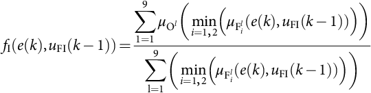
After specifying the fuzzy sets for the fuzzy output variable, FKI, the membership functions for these sets are derived. It is important to note that the same fuzzy singleton membership functions are used here. The control signal of the fuzzy-based integral controller is given by
uFI(k)=GI{fI(e,uFI(k−1))}k∑i=0e(i)Δt,k=0,1,2,…,
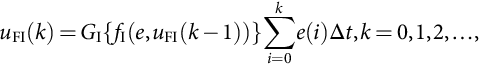
where GI is the scaling factor that is tuned experimentally using genetic optimization.
36.5.3 Fuzzy-Based Derivative Controller
The same process applied to fuzzy-based proportional controller and fuzzy-based integral controller is applied to the fuzzy-based derivative controller. The input signals (state variables) to the controller are e(k) and uFD(k−1)![]() . The output of the controller is the gain FKD. After specifying the fuzzy sets and the membership functions for these sets, the triangle membership functions are also used to define the degree of membership. Figs. 36.2 and 36.3 show the membership functions for the fuzzy sets. Similarly, the linguistic fuzzy output variable “FKD” has nine sets: negative very large (NVL), negative large (NL), negative medium (NM), and negative small (NS), zero (ZE), positive small (PS), positive medium (PM), positive large (PL), and positive very large (PVL). Now, it is necessary to find the final controller output. Consequently, the output of fuzzy-based derivative controller is given by FKD=fD(e(k),uFD(k−1))
. The output of the controller is the gain FKD. After specifying the fuzzy sets and the membership functions for these sets, the triangle membership functions are also used to define the degree of membership. Figs. 36.2 and 36.3 show the membership functions for the fuzzy sets. Similarly, the linguistic fuzzy output variable “FKD” has nine sets: negative very large (NVL), negative large (NL), negative medium (NM), and negative small (NS), zero (ZE), positive small (PS), positive medium (PM), positive large (PL), and positive very large (PVL). Now, it is necessary to find the final controller output. Consequently, the output of fuzzy-based derivative controller is given by FKD=fD(e(k),uFD(k−1))![]() , where
, where
fD(e(k),uFD(k−1))=9∑l=1μOl(mini=1,2(μFli(e(k),uFD(k−1))))9∑l=1(mini=1,2(μFli(e(k),uFD(k−1))))

The control signal of the fuzzy-based derivative controller:
uFD(k)=GDfD(e(k),uFD(k−1))Δe(k)/Δt
where GD is a scaling factor that tuned experimentally using genetic optimization.
Finally, the overall output of fuzzy PID was derived as follows:
uFPID(k)=uFP(k)+uFI(k)+uFD(k)
Saturation is also incorporated in the hybrid fuzzy-PID controller structure. As such, the final output of proposed controller is
umax(k),uFPID(k)>umax(k),u(k)=uFPID(k)umin(k)≤uFPID(k)≤umax(k)umin(k)uFPID(k)<umin(k)(10)
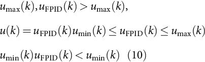
where umin and umax are the permitted minimum and maximum inputs to the brushless drive system.
36.6 Classical PID Versus Fuzzy-PID Controller
The classical linear PID controller in its discrete form can be characterized as
uPID=KPe(k)+KIk∑i=0e(i)Δt+KDΔe(k)/Δtk=0,1,…,
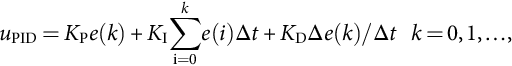
where KP,KI, and KD are constant gains.
This discrete form characterization equation provides a closed-form solution to the proposed fuzzy-PID controller. It can be rewritten as
uFPID(k)=fP(e,DuP)GPe(k)+fI(e,DuI)GIk∑i=0e(i)Δt+fD(e,DuD)GDΔe(k)/Δtk=0,1,2,…=(FKP)eqe(k)+(FKI)eqk∑i=0e(i)Δt+(FKD)eqΔe(k)/Δtk=0,1,2,…,

where (FKP)eq,(FKI)eq, and (FKD)eq are defined to be the equivalent proportional, integral, and derivative gains to a classical linear PID controller, respectively.
36.7 Genetic-Based Autotuning of Fuzzy-PID Controller
Genetic optimization-based approach is used to ensure the best performance of the proposed fuzzy-PID controller. The genetic optimization imitates the natural evolution process in which the fittest survive and the best genes are propagated to the next generation. A population of chromosomes is evaluated and a fitness value is assigned to each. Each chromosome represents a possible solution for a given problem, and the ones with the higher fitness have a better chance to reproduce. One of the main features is that it could work well for nondeterministic systems, ill-defined systems, and systems that are hard to model. Furthermore, the final performance outcome of the algorithm does not depend highly on the initial choice of chromosomes. When the genetic optimization is applied to control applications, each chromosome represents the set of controller's adjustable parameters, and the fitness value is a quantitative measure of the controller performance. The autotuning consists of the automatic adjustment of these parameters to optimize the controller performance. The genetic optimization combines a stochastic exploratory search with a well-defined cost function to find the solution that fit the problem the best. The cost function that represents the fuzzy-PID controller is defined as follows:
J=F(GP,GI,GD),
where GP,GI,GD are the output scaling factors of the fuzzy-PID subcontrollers. The function F represents the relationship between the overall performance and the design parameters.
The optimization problem for the fuzzy-PID controller is described as
max(F(GP,GI,GD))=max(1/J)
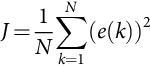
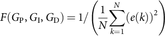
where F is the fitness function. There are various ways to calculate the overall performance J of the controller, but for simplicity reasons, the mean square error (MSE) performance index was selected.
J=1NN∑k=1(e(k))2
where N is the length of the evaluation window and e(k) is the error between the reference speed and the actual speed. The fitness of each parameter set or chromosome can be determined as follows:
F(GP,GI,GD)=1/(1NN∑k=1(e(k))2)
Once the fitness function is established, the genetic operators and parameters are defined. The genetic optimization consists of three basic operators: the crossover, mutation, and reproduction. The parameters are the number of generations, the population size, the probability of crossover, and mutation. In general, an initial population size is defined and evaluated with the fitness function. Once each chromosome has a fitness assigned to it, the reproduction process takes place with those that are more fit having a greater chance to be selected. Then, each of the two operators of crossover and mutation is applied to create the new pool of chromosomes to be evaluated. Crossover occurs when the chromosomes partially exchange their information by interchanging some of their genes. Mutation is the random alteration of a particular section of the chromosome by occasionally changing one or more of the genes that are part of the chromosome. For this optimization task, a crossover factor of 0.3 and a mutation factor of 0.7 were used. Another important aspect of the genetic optimization is the coding of the parameters. Binary coding has been used widely for decades; however, real-coded algorithms are proving useful for a number of applications, and it was chosen to implement the genetic optimization algorithm. One of the difficulties of the real-time implementation is in the simultaneous evaluation of the fitness for all the chromosomes in one generation as a batch data. This problem was overcome by reducing the population size to one and evaluating the fitness function of each chromosome sequentially. The mutation function is applied by increasing or decreasing the value proportional to a uniformly distributed random number between −0.9 and 1. The crossover is implemented with the chromosome that had the higher value for the fitness function and the chromosome being tested in the current generation. A Bernoulli binary set of numbers with probability of 0.5 is used to select the resulting offspring chromosome with a mix of genes from both parent chromosomes. The overall genetic-based autotuning procedure of the fuzzy-PID controller consists of the following steps:
Step 1: Select the control topology of the fuzzy-PID controller in which the outputs of the subcontrollers are used as the FPID gains.
Step 2: Define the characteristics of the fuzzy-PID subcontrollers such as the number of fuzzy sets, membership functions, fuzzy rules, and defuzzification method.
Step 3: Set the genetic optimization parameters, such as the number of generations, the population size, the probability of crossover, and mutation.
Step 4: The last step is the tuning of the parameters, GP,GI, and GD of the fuzzy-PID controller using the genetic optimization procedure.
36.8 Fuzzy and H∞ Control Design
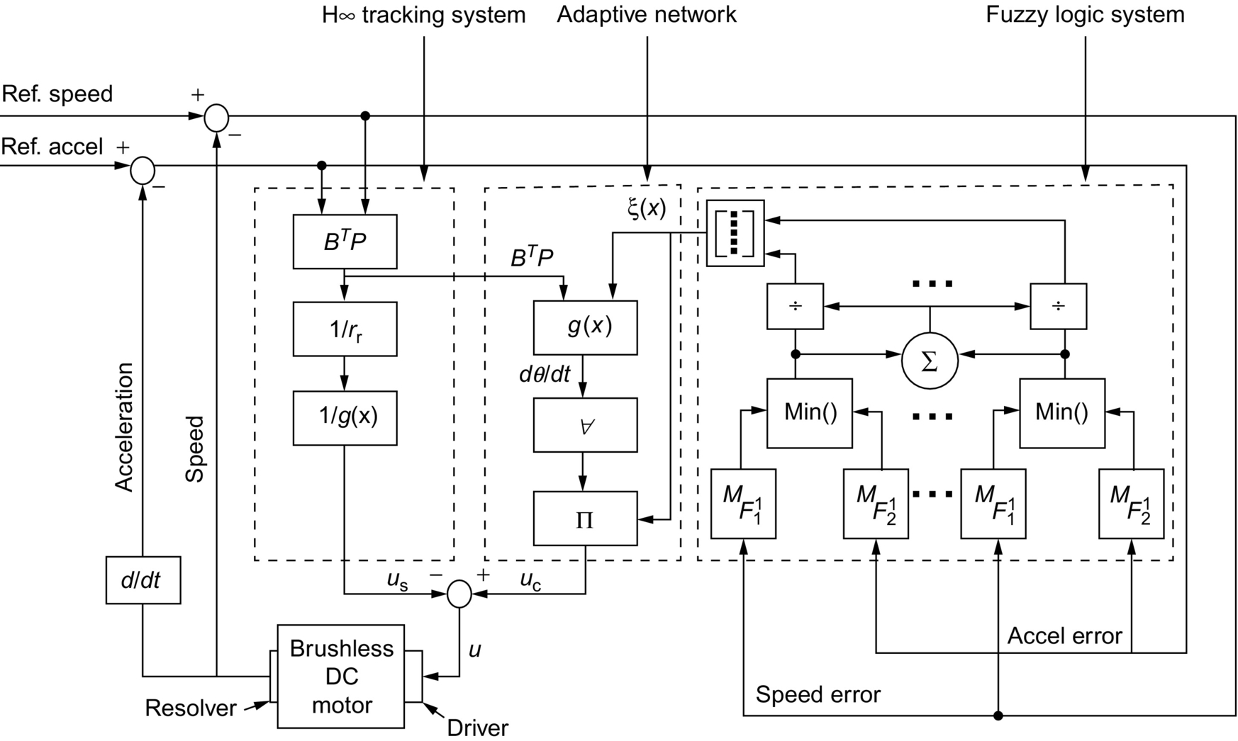
36.8.1 Brushless Servo-Motor Drive System
The brushless DC motor used in the section is excited by a three-phase sinusoidal supply and driven from a six-step inverter, which converts a constant voltage to a three-phase voltage with a frequency corresponding instantaneously to the rotor speed. The model of the drive system is used to design the H∞![]() tracking controller and to simulate its dynamic behavior. However, fuzzy-logic controller does not require mathematical models and has the ability to approximate nonlinear systems. The reader is referred to [16] for details of the dynamic model of the brushless dc motor drive system. For the purpose of discussion, the dynamics of the brushless servomotor drive system can be written in state space form as follows:
tracking controller and to simulate its dynamic behavior. However, fuzzy-logic controller does not require mathematical models and has the ability to approximate nonlinear systems. The reader is referred to [16] for details of the dynamic model of the brushless dc motor drive system. For the purpose of discussion, the dynamics of the brushless servomotor drive system can be written in state space form as follows:
x(n)=f(x)+Bu+d
where x=(x,.x,…,x(n−1))T∈Rn![]() , d is the external disturbance, and B≠0
, d is the external disturbance, and B≠0![]() . Since B≠0
. Since B≠0![]() for x∈Rn
for x∈Rn![]() , the system is controllable in the whole space Rn.
, the system is controllable in the whole space Rn.
36.8.2 The Fuzzy H∞ Control Structure
A hybrid adaptive fuzzy controller is implemented, which employs a fuzzy-logic controller integrating an H∞![]() tracking controller. The H∞
tracking controller. The H∞![]() tracking controller is capable of taking care of the robust stabilization and disturbance rejection problems, while fuzzy-logic controller is used as principle components of the adaptive fuzzy controller. Actually, it is outfitted with an adaptive control law that modifies the parameters of the controller based on a Lyapunov synthesis approach. Fig. 36.13 shows the block diagram of the proposed control structure.
tracking controller is capable of taking care of the robust stabilization and disturbance rejection problems, while fuzzy-logic controller is used as principle components of the adaptive fuzzy controller. Actually, it is outfitted with an adaptive control law that modifies the parameters of the controller based on a Lyapunov synthesis approach. Fig. 36.13 shows the block diagram of the proposed control structure.
36.8.3 H∞ Control Design
The controller objective is to obtain high-performance servo tracking; therefore, the control problem is to force the actual output to follow a predetermined bounded reference trajectory. The tracking performance indicates how closely the servomotor follows a desired position trajectory, velocity trajectory, or acceleration trajectory. For the purpose of discussion, we define the tracking error to be ˉɛ=[ɛ,.ɛ]T![]() , where ɛ is the rotor speed error and .ɛ
, where ɛ is the rotor speed error and .ɛ![]() is the acceleration error. Consequently, the motor speed error ɛ=ωref−ωact
is the acceleration error. Consequently, the motor speed error ɛ=ωref−ωact![]() and the acceleration error .ɛ=αref−αact
and the acceleration error .ɛ=αref−αact![]() are used as input variables to the H∞
are used as input variables to the H∞![]() controller. Here, ωact is the actual speed in rev/s, ωref is the desired reference speed, αref is the desired acceleration in rev/s2, and αact is the calculated acceleration. The acceleration is calculated as the difference in the speed over two successive sampling periods. A block diagram of the H∞
controller. Here, ωact is the actual speed in rev/s, ωref is the desired reference speed, αref is the desired acceleration in rev/s2, and αact is the calculated acceleration. The acceleration is calculated as the difference in the speed over two successive sampling periods. A block diagram of the H∞![]() tracking controller is shown in Fig. 36.14. The H∞
tracking controller is shown in Fig. 36.14. The H∞![]() control law is defined as [17]
control law is defined as [17]

 tracking controller.
u∞=−1rrBTPɛ
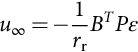
where rr is a weighting factor and P is the solution of the simplified Riccati-like equation for P=PT≥0![]()
PA+ATP=−Q
The matrices A and B are given by
A=[01−k2−k1]B=[01]
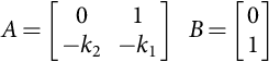
where k=[k1,k2]![]() is chosen such that all roots of the polynomial p(S)=Sn+KnSn−1+⋯+k1
is chosen such that all roots of the polynomial p(S)=Sn+KnSn−1+⋯+k1![]() are in the open left-hand plane.
are in the open left-hand plane.
36.8.4 Fuzzy Logic Control Design
The fuzzy-logic principles with center-average defuzzifier, product inference, and singleton fuzzifier are used as building blocks for the fuzzy controller. A block diagram of the fuzzy control structure is shown in Fig. 36.15. The fuzzy-logic-based controller implemented in this work has two inputs and one output. The inputs are the rotor speed error and the feedback acceleration error, with each of these inputs corresponding to a fuzzy variable.
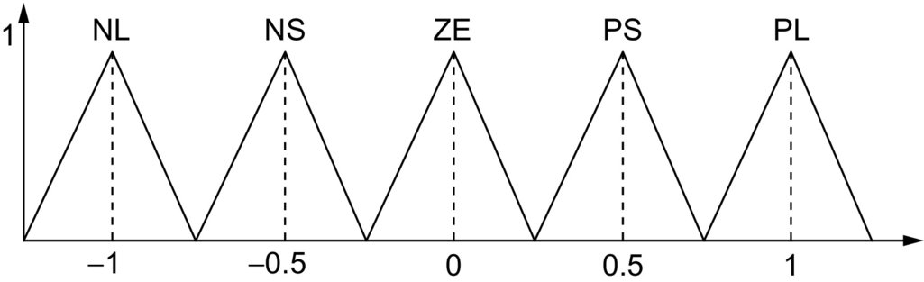
The output is the fuzzy control decision. The fuzzy variable associated with the rotor speed error signal consists of five fuzzy sets: positive large (PL), positive medium (PM), zero (ZE), negative large (NL), and negative medium (NM). Typical example of the fuzzy membership functions used for the speed is shown in Fig. 36.16. In this way, for any given value of the rotor angle, the degree of membership μ, to which it belongs to each of these sets, can be determined, and a control decision based on this information can be obtained.
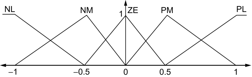
Similarly, the acceleration error can be described by a group of partially overlapping fuzzy sets as positive large (PL), positive medium (PM), zero (ZE), negative large (NL), and negative medium (NM), with each set having its own membership function. An example of typical membership functions that make up the fuzzy variable acceleration is shown in Fig. 36.17.

The five fuzzy sets can be symbolized by FjI,i=1,2![]() and j=1,2,3…5
and j=1,2,3…5![]() . Their membership functions can be symbolized by μFjI(xI),i=1,2
. Their membership functions can be symbolized by μFjI(xI),i=1,2![]() and j=1,2,3…5
and j=1,2,3…5![]() .
.
36.8.5 Fuzzy Logic Rules
The next step in the design of the fuzzy-logic-based controller is the determination of the fuzzy IF-THEN inference rules. The number of fuzzy rules that are required is equal to the product of the number of fuzzy sets that make up each of the two fuzzy input variables. For the fuzzy controller described here, the input variables representing the rotor speed and its acceleration consist of five fuzzy sets each. Thus, a total of 25 fuzzy rules are required. During each sampling interval that a controller is calculated, the present value of the degree of membership of the motor speed and its acceleration is calculated for each of the fuzzy sets that make up their respective fuzzy variables. This process is one of the largest computational burdens of the fuzzy-logic control algorithm if each fuzzy set is expected to have some degree of membership for the present input value of the motor speed and its acceleration. This will in addition affect the computational speed at which the fuzzy rules are processed since all the rules have to be evaluated.
Using a triangular membership function for the input variables was very desirable to reduce this computational burden and speed up the process. This ensures that only two fuzzy sets, which are overlapping, will actually have a nonzero degree of membership (Figs. 36.16 and 36.17). With this advantage, the evaluation of the degree of membership in each set is accelerated. This also speeds up the evaluation of the fuzzy rules since only those rules that correspond to nonzero values of membership function need to be evaluated. Hence, for this controller, only four fuzzy rules need to be evaluated during any sampling interval. The fuzzy inference rules have been determined experimentally using the measured responses of the brushless drive servo system. A typical fuzzy rule is of the form:
[R(1):] IF x1 is F1j, and x2 is F2j, THEN O is G1l for j=1…5,l=1…5![]() .
.
In general,
[R(k):] IF x1 is F1j, and x2 is F2j, THEN O is Gkl for j=1…5,l=1…5,k=1…25![]() .
.
The conjunction of the rule antecedents is evaluated by the fuzzy operation intersection, which is implemented by the min operator. The rule strength represents the degree of membership of the output variable for a particular rule. Defining the rule strength, ξi,j, of a particular rule as
ξi,j=min(μFspeedi,μFaccelj)
where i∈[PL,PM,ZE,NM,NL]![]() is associated with the fuzzy variable, speed, and j∈[PL,PM,ZE,NM,NL]
is associated with the fuzzy variable, speed, and j∈[PL,PM,ZE,NM,NL]![]() is associated with the fuzzy variable, acceleration. From above, it is clear that for all the rules where at least one of the degrees of membership in the corresponding fuzzy sets is zero, the output of the min operator will be zero, and hence, these rules do not have to be analyzed. The fuzzy inference engine uses the appropriately designed knowledge base to evaluate the fuzzy rules and produce an output for each rule. Subsequently, the multiple outputs are transformed to a crisp output by the defuzzification interface.
is associated with the fuzzy variable, acceleration. From above, it is clear that for all the rules where at least one of the degrees of membership in the corresponding fuzzy sets is zero, the output of the min operator will be zero, and hence, these rules do not have to be analyzed. The fuzzy inference engine uses the appropriately designed knowledge base to evaluate the fuzzy rules and produce an output for each rule. Subsequently, the multiple outputs are transformed to a crisp output by the defuzzification interface.
36.8.6 Defuzzification
Once the aggregated fuzzy set representing the fuzzy output variable has been determined, an actual crisp control decision must be made. The process of decoding the output to produce an actual value for the control signal is referred to as defuzzification. Thus, a fuzzy-logic controller-based center-average defuzzifier is implemented. The control output can be written in general form:
O(x)=25∑l=1μOl(mini=1,2(μFli(x)))/25∑l=1(mini=1,2(μFli(x)))
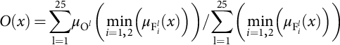
which can be written in the form
O(x)=θTξ(x)=ξT(x)θ
where
ξl(x)=mini=1,2(μFli(x))/25∑l=1(mini=1,2(μFli(x)))

θ=(μO1,…μO25,)![]() is a parameter vector representing the degree of membership of the output, which is tuned online using an adaptation law.
is a parameter vector representing the degree of membership of the output, which is tuned online using an adaptation law.
36.8.7 On-Line Adaptation
By using an adaptive law, the fuzzy parameters, θ, can be tuned online based on the Lyapunov synthesis approach. The feedback control law can be expressed as follows [17]:
u=ξT(x)θ−u∞/g
where θ is a vector denoting the parameter estimate of fuzzy-logic controller. The parameter θ is adjusted using the following adaptive law:
.θ=γξ(x)gBTPɛ
where γ is an adaptation gain and g is a constant that depends on machine parameters. A block diagram of the hybrid adaptive fuzzy controller is shown in Fig. 36.18.
 control structure.
36.9 Fuzzy Control for DC-DC Converters
36.9.1 Background
The DC-DC converters are generally divided into two groups: hard-switching converters and soft-switching converters. In hard-switching converters, the power switches cut off the load current within the turn-on and turn-off times under the hard-switching conditions. The output voltage is controlled by adjusting the on-time of the power switch, which in turn adjusts the width of a voltage pulse at the output. This is known as PWM control. In soft-switching converters, resonant components are used to create oscillatory voltage or current waveforms so that the zero-voltage switching or zero-current switching conditions could be created for the power switches. For many years, control design for converters has been carried out through analog circuits, which limited them to mostly PI controller structure. The PI controllers generally give overshoot in output voltage and high initial current when rise time of response is reduced. Feed-forward types of controllers have also been designed by sensing the input voltage to improve line regulation in applications with a wide range of input voltages and load currents. However, direct sensing of the input voltage through a feed-forward loop may induce large-signal disturbances that could upset the normal duty cycle of the converter. Using human linguistic terms and common sense, several fuzzy-logic controllers have been developed and implemented for the DC-DC converters [18–20]. These controllers have shown promise in dealing with nonlinear systems and achieving voltage regulation in buck converters. Fuzzy-logic control uses humanlike linguistic terms in the form of IF-THEN rules to capture the nonlinear system dynamics. Once in place, the fuzzy rules will not be able to adapt themselves to adequately capture the dynamics and external disturbances of the converter. Although achieving many practical successes, fuzzy control has not been viewed as a rigorous science due to a lack of formal analysis and synthesis techniques. As a result of this, a lot of work has been done to develop adaptive fuzzy controllers and automate the modeling process as much as possible. Recently, the resurgence of interest in ANN has injected a new driving force into fuzzy literature. One of the major features of ANNs is their learning capability. A learning algorithm is usually used to update the nonlinear parameters of the network architecture. A drawback in using an ANN for control is that there is so much freedom in structural implementation choice that it is often difficult to decide how complex a structure is actually necessary for the desired control. Besides, the implementation is not at all intuitive, and the inner workings of the network are very much invisible to the designer. The integration of neural network architectures with fuzzy inference system has resulted in a very powerful strategy known as adaptive network-based fuzzy inference system. Some researchers suggest that neural networks and fuzzy control are in fact special instances of adaptive networks [21,22]. The suggested fuzzy inference system has the advantage that it can not only take linguistic information from human experts but also adapt itself using numerical data to achieve better performance.
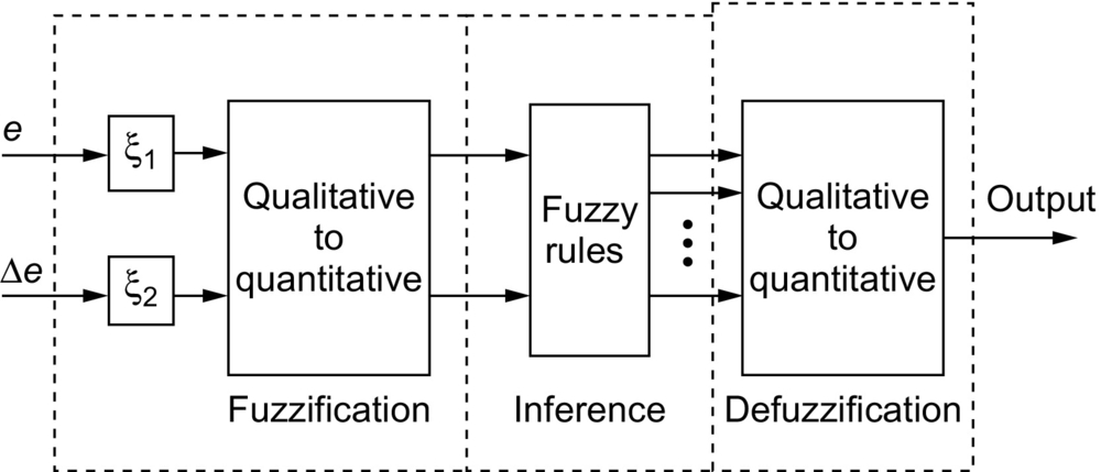
36.10 Fuzzy Control Design for Switch-Mode Power Converters
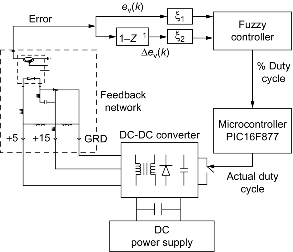
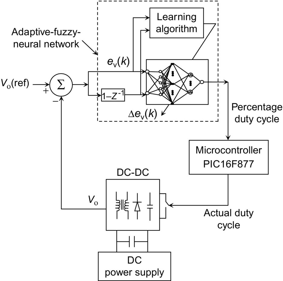
The structure built-up here is a two-input single-output controller. The inputs are the variable voltage error, e(k), and the change in voltage error, Δe(k). Consequently, the input to the DC-DC converter would be the duty cycle that is actually the output of the fuzzy controller. The operational structure of the proposed fuzzy controller is shown in Fig. 36.19. It consists of three building blocks: (1) a fuzzification block that expresses quantitative action to qualitative action, (2) fuzzy inference engine that generates the fuzzy rules, and (3) a defuzzification block that articulates qualitative action to quantitative action. Fuzzification translates a numeric value for the error e(k) or change in error Δe(k) into a linguistic value such as big or small with a membership grade. Defuzzification takes the fuzzy output of the rules and generates a “crisp” numeric value used as the control input to the DC-DC converter. The controller qualitatively captures the dynamics of the DC-DC converter and executes this qualitative idea in a real-time situation. The DC-DC converter is equipped with a feedback network that provides the error value at the output. The overall architecture of a DC-DC converter topology with the fuzzy controller structure is given in Fig. 36.20. The feedback network consists of a precision voltage reference with a nominal voltage of 2.5 V. The 5 and 15 V output potentials are combined in a resistive sampling network in such a way that the output voltage of the network is 2.5 V when the potentials are closed to their nominal magnitudes. This output voltage is then compared internally with the reference of the precision voltage reference, and any error difference detected is amplified and fed back. The converter is represented by a “black box” from which we only extract the terminals corresponding to input voltage (VI), output voltage (Vo), and controlled switch (S). From these measurements, the controller provides a percentage duty-cycle signal for a peripheral interface microcontroller PIC16F877, which generates the converters' actual duty cycle.
36.10.1 DC-DC Switch-Mode Power Converter
The DC-DC switch-mode power converter consists of six distinct circuit networks as shown in Fig. 36.21, working together to form a complete DC-to-DC dual-output switch-mode power regulator [23]. The six distinct circuit networks are (1) the bias voltage regulator network, (2) the 100 KHZ clock, (3) the pulse-width modulator (PWM), (4) the power switch driver interface, (5) the feedback error amplifier, and (6) the integrated-magnetic (IM) power stage. In order to implement the proposed adaptive fuzzy-neural-network controller, the converter system shown in Fig. 36.21 was modified by removing the bias voltage regulator network, the 100 KHz clock, and the pulse-width modulator (PWM), which is the core of the control system. The power-stage concept is based on that of a “dual-output forward” configuration operating in a continuous mode of energy storage. When the power MOSFET switch Q1 is turned ON, energy is transferred from the input power source (VIN) to the two secondary sides of the transformer. The voltage potential across the terminals of C1 will be that of the reflected line voltage, namely, NS1×VIN/NP![]() . The ON time is a fraction of the clock period, and it has to be short and long enough to bring the output to a level above the desired voltage (5 and 15 V). Diodes D1 and D4 conduct allowing the energy transfer to be used to supply 5 and 15 V load power, respectively, and to replenish the energy lost in the “output” inductors during the previous OFF period of Q1. Diodes D2 and D3 do not conduct during this time, since they are reverse-biased.
. The ON time is a fraction of the clock period, and it has to be short and long enough to bring the output to a level above the desired voltage (5 and 15 V). Diodes D1 and D4 conduct allowing the energy transfer to be used to supply 5 and 15 V load power, respectively, and to replenish the energy lost in the “output” inductors during the previous OFF period of Q1. Diodes D2 and D3 do not conduct during this time, since they are reverse-biased.

When Q1 turns OFF, the 5 and 15 V load power is sustained by the energies of the two “inductors” (L1 and L2). The output stored energy, located in two inductors, will then start discharging causing the voltages to drop. Diodes D2 and D3 conduct during this time with diodes D1 and D4 forced off. As soon as the voltages go below the desired values, another impulse will be applied on Q1 (Q1 ON), to bring the voltage back upward. Capacitors C2 (0.001 μf) and C3 (100 μf) serve to prevent the dynamic ripple currents in the “inductors” from appearing at the 5 and 15 V load terminals, respectively.
36.11 Optimum Topology of the Fuzzy Controller
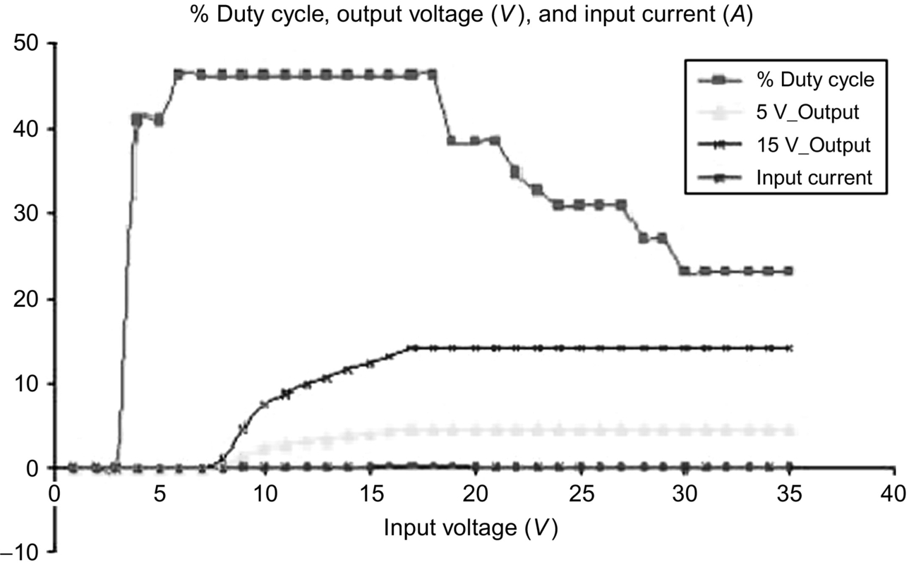
The main problem with fuzzy controller generation is related to the definition of its optimum topology such as scaling factors, number of fuzzy sets, shape of the fuzzy sets, and decision-making. This section is devoted to the topology determination of the proposed fuzzy controller structure. Various test cases were performed on the DC-DC converter in order to determine the ranges of membership functions and other system-specific responses of the converter that will help in the design of the linguistic control rules of the proposed controller. The experimental tests were focused on the responses of the DC-DC converter with and without the action of the controller. One other point was to observe how the changes of the control signal and the variations of the error signal with respect to the variations of the input voltage. The various voltage ranges observed in the test cases assisted in choosing the ranges for the input and output membership set. A summary of some of these tests is shown in Figs. 36.22–36.24. Fig. 36.22 shows the optimum trajectories of the duty cycle, the output voltage, and the input current with variations in the input voltage. From Fig. 36.22, when the input voltage increases, the control signal pulses get reduced to maintain the output voltages at their required level. The other information gives the range of the control signal (i.e., 16%–50%) required for the working range of the DC-DC converter. A similar test case was conducted while the error of the system was observed. Fig. 36.23 shows four different test cases of variations of the error voltage and duty cycle with increase in the input voltage plotted together. The figure shows four variations of the error voltage with the control signal at 16%, 24%, 32%, and 40% duty cycle. For the 40% duty-cycle test case, the feedback network becomes active at an input voltage of 18 V. When the duty cycle was reduced to 32%, the feedback network becomes active at around 21 V of the input voltage. At 16% duty cycle, it was realized that the feedback network was not yet active at 36 V of the input voltage. This test case shows that when the feedback network is active, the error voltages are all below 2 V. Fig. 36.23 also gives the actual values of the error voltage and the control signals needed at each stage of the input voltage variations. A general rule from Fig. 36.23 will be “if the error voltage is high (i.e., max 6 V) and the change in error is zero (i.e., very small), then increase the control signal (i.e., duty cycle).” In Fig. 36.24, a 5 V output voltage level was tested for different constant control signals while increasing the input voltage. Four different test cases were conducted for duty-cycle values of 16%, 24%, 32%, and 40%. From the figure, it shows the various voltage levels at which the output voltage gets to the 5 V mark for the different duty cycles. It also shows that without any control, the output voltage will continue to increase without any bound. These experimental observations were in general very helpful in the design of the fuzzy-logic controller.


36.11.1 Membership Functions and Rules Generation
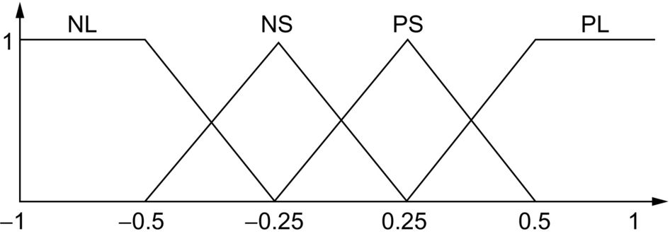
The chief problem of the construction of the fuzzy controller is related to the choice of the regulator parameters. Certainly, there is no systematic procedure for the design of a fuzzy controller (membership functions and rules generation), and this section is devoted to the determination of the fuzzy sets and the linguistic rules. The number of the linguistic sets of the proposed controller has been determined using laboratory experimentation and the responses of the DC-DC converter that have been compared with different numbers of the fuzzy sets. The actual responses have been compared with three, four, five, and seven fuzzy sets. It has been found that the use of more than five linguistic sets does not improve the tracking accuracy of the DC-DC converters but in fact increases the computation time. Consequently, four linguistic sets, positive large (PL), positive small (PS), negative large (NL), and negative small (NS), have been chosen for the input variable voltage error, e(k), and three linguistic sets, positive medium (PM), zero (ZE), and negative medium (NM), have been chosen for that of the change in voltage error, Δe(k). Additionally, five linguistic sets, positive large (PL), positive small (PS), zero, negative large (NL), and negative small (NL), have been chosen for the output variable of the fuzzy controller structure. The fuzzy controller utilizes triangular membership functions on the controller input. The triangular membership function is chosen owing to its simplicity. For the change in voltage error, Δe(k), the initial values of the premise parameters (the corner coordinates of the triangle) are chosen so that the membership functions are equally spaced along the operating range of each input variable. The scaled input and output membership functions sets are shown in Figs. 36.25 through 36.27. The actual error measured from the feedback network ranges from 0.8 to about 6.0 V, while the control signal ranges from 16% to 50% duty cycle. The scaling factors ξ1=0.167![]() and ξ2=0.01
and ξ2=0.01![]() were determined using experimental tests in such a way that the normalized inputs e(k) and Δe(k) are well adapted to the universe of discourse [−1,1]
were determined using experimental tests in such a way that the normalized inputs e(k) and Δe(k) are well adapted to the universe of discourse [−1,1]![]() for any operating point. The linguistic control rules are established considering the dynamic behavior of the DC-DC converter and analyzing the error and its variation. To obtain control decision, the max-min inference method is used. It is based on the minimum function to describe the “AND” operator present in each control rule and the maximum function to describe the “OR” operator.
for any operating point. The linguistic control rules are established considering the dynamic behavior of the DC-DC converter and analyzing the error and its variation. To obtain control decision, the max-min inference method is used. It is based on the minimum function to describe the “AND” operator present in each control rule and the maximum function to describe the “OR” operator.
The output of the fuzzy controller structure is crisp, and thus a combined output fuzzy set must be defuzzified. To express the qualitative action in a quantitative action, the sum-product composition method was used. It calculates the crisp output as the weighted average of the centroids of all output membership functions. The output of the controller can be expressed as
Oo=(∑mO∗maCm×bCm)∑m(O∗mbCm)
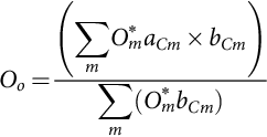
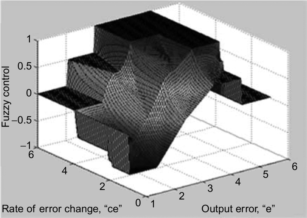
where aCm and bCm are the centers and widths of the output fuzzy sets, respectively, for m=1,…,5![]() . The values of the bCm s were chosen to be unity. This scaled output corresponds to the control signal (percent duty cycle) to be applied to maintain the output voltage at a constant value. Fig. 36.28 represents the normalized output Oo of the proposed fuzzy controller structure as a function of the error e(k) and the change of error Δe(k). It clearly illustrates the nonlinear characteristics of the proposed fuzzy controller structure.
. The values of the bCm s were chosen to be unity. This scaled output corresponds to the control signal (percent duty cycle) to be applied to maintain the output voltage at a constant value. Fig. 36.28 represents the normalized output Oo of the proposed fuzzy controller structure as a function of the error e(k) and the change of error Δe(k). It clearly illustrates the nonlinear characteristics of the proposed fuzzy controller structure.
36.12 Adaptive Network-Based Fuzzy Control System for DC-DC Converters
Adaptive network architecture, ANFIS, and a learning algorithm by which the ANFIS could construct a desired input-output mapping are proposed. The basic structure of a converter topology with adaptive network architecture is given in Fig. 36.29. Both fuzzy-logic principles and learning functions of neural networks are employed together to construct the adaptive fuzzy-network inference system for the control topology. Initially, a basic fuzzy-logic controller is set up utilizing linguistic rules, and then numerical data is used for training the controller. The number of membership functions is chosen so as to cover the entire input space. The converter is represented by a “black box” from which we only extract the terminals corresponding to input voltage (Vi), output voltage (Vo), and controlled switch (S). From these measurements, the ANFIS provides a signal proportional to a percentage duty-cycle signal for a peripheral interface microcontroller, PIC16F877, which generates the converters' actual duty cycle.
36.12.1 Topology of the Neural-Fuzzy Controller (NFC)
The proposed ANFIS is a multilayer neural network-based fuzzy-logic controller. The network architecture is built, such that the designer recognizes the internal nodes as they relate to the components of fuzzy controller. The system has a total of five layers. The architecture of the network is shown in Fig. 36.30. The scaled input and output membership functions sets are shown in Figs. 36.3–36.5. The actual error measured from the feedback network ranges from 0.8 to about 6.0 V, while the control signal ranges from 16% to 50% duty cycle.

36.12.1.1 Layer 1: Input Layer
Each node in this layer is an input node, which corresponds to one input variable. These nodes only bypass input signals to the next layer. The input variables are the output voltage error e(k)=Vo(k)−Voref(k)![]() and change in voltage error Δe(k)=[e(k)−e(k−1)]
and change in voltage error Δe(k)=[e(k)−e(k−1)]![]() , respectively. The fuzzy sets proposed for the input variable voltage error, e(k), are positive large (PL), positive medium (PM), positive small (PS), and small (S) and that for the change in voltage error, Δe(k), are positive medium (PM), zero (ZE), and negative medium (NM). The output of the neuron i in layer 1 is obtained as
, respectively. The fuzzy sets proposed for the input variable voltage error, e(k), are positive large (PL), positive medium (PM), positive small (PS), and small (S) and that for the change in voltage error, Δe(k), are positive medium (PM), zero (ZE), and negative medium (NM). The output of the neuron i in layer 1 is obtained as
O1i=f1i(net1i)=net1i
where netI1 is the ith input to the node of layer 1, namely, the error and the change in the error.
36.12.1.2 Layer 2: Input Membership Layer
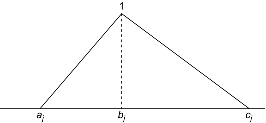
Each node in this layer acts as a linguistic label of one of the input variables in layer 1, that is, the membership value specifying the degree to which an input value belongs to a fuzzy set is determined in this layer. The triangular membership function is chosen owing to its simplicity. For the change in voltage error, Δe(k), the initial values of the premise parameters (the corner coordinates of the triangle) are chosen so that the membership functions are equally spaced along the operating range of each input variable. Due to the nonlinearity in the converter, the triangular membership for the error, e(k), was slightly modified. The weights between the input and membership level are assumed to be unity. The output of neuron j in the second layer can be obtained as follows:
when (Xi≥aj)and(Xi≤bj)![]()
O2j=f2j(net2j)=(Xi−aj)/(bj−aj)
else when (Xi≥bj)and(Xi≤cj)![]()
O2j=f2j(net2j)=(Xi−cj)/(bj−cj)
where aj,bj, and cj are the corners of the jth membership function in layer 2 shown in Fig. 36.31 and Xi is the ith input variable to the node of layer 2, which could be either the value of the error or the change in error.
36.12.1.3 Layer 3: Rule Layer
Each node in layer 3 multiplies the incoming signal and outputs the result of the product. The conjunction of the rule antecedents is evaluated by the fuzzy operation intersection, which is implemented by the product operator. Consequently, each node of this layer is a rule node that represents one fuzzy control rule. Each node takes two inputs: one from nodes A1–A4 and the other from nodes B1–B3 of layer 2. Nodes A1–A4 define the membership values for the voltage error, and nodes B1–B3 define the membership values for the change in voltage error. Accordingly, there are 12 nodes in layer 3 to form a fuzzy rule base for two input variables, with four linguistic variables for the input voltage error, e(k), and three linguistic variables for the input change in voltage error, Δe(k). The input/output links of layer 3 define the preconditions and the outcome of the rule nodes, respectively. The outcome is the strength applied to the evaluation of the effect defined for each particular rule. The output of neuron k in layer 3 is obtained as
O3k=f3k(net3k)=net3k,wherenet3k=∏jw3jky3j
yj3 represents the j th input to the node of layer 3, and wjk3 is assumed to be unity.
36.12.1.4 Layer 4: Output Membership Layer
Neurons in this layer represent fuzzy sets used in the consequent of fuzzy rules. An output membership neuron receives inputs from the corresponding fuzzy rule neurons and combines them by using the fuzzy operation union. This was implemented by the maximum function. Layer 4 acts upon the output of layer 3 multiplied by the connecting weights. These link weights represent the output action of the rule nodes evaluated by layer 3. That output is given by
O4m=f4m(net4km)=max(net4km)
and
net4km=O3kwkm
where the count of k depends on the links from layer 3 to the particular mth output in layer 4 and the link weight wkm is the output action of the mth output associate with the kth rule. This level is essential in ensuring the system's stability and allowing a smooth control action.
36.12.1.5 Layer 5: Defuzzification Layer
Layer 5 is the output layer and acts as a defuzzifier. The single node in this layer takes the output fuzzy sets clipped by the respective integrated firing strengths and combines them into a single fuzzy set. The output of the neurofuzzy system is crisp, and thus a combined output fuzzy set must be defuzzified. The sum-product composition method was used. It calculates the crisp output as the weighted average of the centroids of all output membership functions.
Oo=f5o(net5o)=net5o
and
net5o=(∑mO4m×aCm×bCm)∑m(O4m×bCm)

where aCm and bCm for m=1,…,5![]() are the centers and widths of the output fuzzy sets, respectively. The values for the bCm’s were chosen to be unity. This scaled output corresponds to the control signal (percent duty cycle) to be applied to maintain the output voltage at a constant value.
are the centers and widths of the output fuzzy sets, respectively. The values for the bCm’s were chosen to be unity. This scaled output corresponds to the control signal (percent duty cycle) to be applied to maintain the output voltage at a constant value.
36.12.2 Learning Algorithm
The only weights that are trained are those between layer 3 and layer 4 of Fig. 36.30. The back-propagation network is used to train the weights of this layer. The weights of the neural network were trained offline before they were used in the experimental setup. The learning algorithm used can be described in the following steps:
Step 1: Calculate the error for the change in the control signal (duty cycle) based on the type of the converter.
Eo=To−O5o
where Eo,To, and Oo5 are the output error, the target control signal, and the actual control signal, respectively.
Step 2: Calculate the error gradient.
δm=Eo×f′(O41,…,O4m)⇒δm=(To−O5o)×f′(O41,…,O4m)
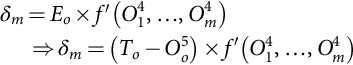
where
f(O41,…,O4m)=m∑j=1O4j×aCjm∑j=1O4j
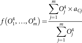
and the partial derivative of f with respect to Om4 is given by
fO4m′(O41,…,O4m)=m−1∑j=1j≠mO4j×(aCm−aCj)(m∑j=1O4j)2

where aCi for i=1,…,5![]() are the centers of the output fuzzy sets and Oj4 is the firing strength from node j in layer 4.
are the centers of the output fuzzy sets and Oj4 is the firing strength from node j in layer 4.
Step 3: Calculate the weight correction
Δwkm=η×δm×O3k
to increase the learning rate, the Sejnowski-Rosenberg updating mechanism was used, which takes into account the effect of past weight changes on the current direction of the movement in the weight space. This is given by
Δwkm(t)=η×(1−α)×δm×O3m+α×Δwkm(t−1)
where α is a smoothing coefficient in the range of 0–1.0 and η is the learning rate.
Step 4: Update the weights.
wkm(t+1)=wkm(t)+Δwkm(t)
where t is the iteration number
The weights linking the rule layer (layer 3) and the output membership layer (layer 4) are trained to capture the system dynamics and therefore minimize the ripples around the operating point. The training results of the link weights are shown in Figs. 36.32 and 36.33.
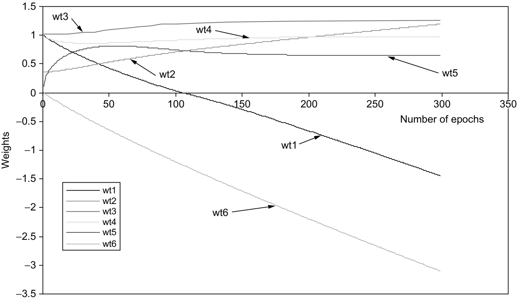
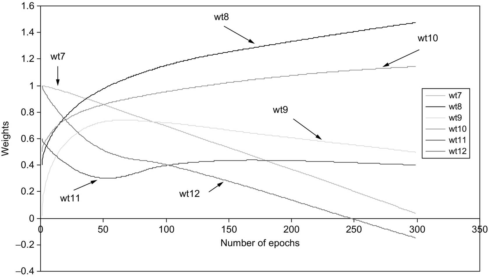
In the initialization of the weights, wt5 and wt6 in Fig. 36.32 were set to a very small number of 0.001 with the initial assumption that those weights are almost redundant before the training begins. However, the neurofuzzy system was capable of correcting those assumptions. Weight wt5 finally converges to a positive value that indicates an excitatory rule weight, while wt6 converges to a negative number that is an inhibitory rule weight. Some of the weights change sign during the training process. Weight wt1 was initially set at a positive value but converges to a negative value that makes that rule weight inhibitory.
36.13 Summary
The presence of adaptive control via the EKF learning of the FNN control laws marks an improvement over the FL design. The motor drive over time is subject to experience degradation of mechanical parts or even electric characteristics, and the ability to automatically adapt the control laws to these changes is a feature that a nonadaptive fuzzy controller does not have. A genetic-based FPID controller and its integration with a classical PID in a global control scheme have been developed. Experimental results have shown excellent tracking performance of the proposed hybrid FPID controller and have convincingly demonstrated the usefulness of the FPID controller in high-performance drives with uncertainties. For the H-infinity-based controller, test results have shown that the proposed hybrid controller achieved good tracking performance and stable control, under loading conditions for a number of desired reference trajectories. The ability of the hybrid controller to achieve the tracking process with a high degree of accuracy, even in the presence of random disturbance, was also demonstrated, while the fuzzy application to the DC-DC converter topology showed considerable control performance over a wide range of operating conditions.