
Multiphase Converters
Atif Iqbal Qatar University, Doha, Qatar
Shaikh Moinoddin Aligarh Muslim University, Aligarh, India
Salman Ahmad Aligarh Muslim University, Aligarh, India
Mohammad Ali Aligarh Muslim University, Aligarh, India
Adil Sarwar Aligarh Muslim University, Aligarh, India
Kishore N. Mude University of Porto, Porto, Portugal
Amrita Vishwa Vidyapeetham University, Bengaluru, India
Abstract
Multiphase converters refer to converters with more than three phases and are the extension of three-phase converters by adding extra legs. From hardware point of view, as such there is no major difference between a three-phase and a multiphase converter except the number of legs. However, control becomes more flexible and complex, and higher degrees of redundancies are available. Multiphase power converters have gained popularity in the last decade because of the developments in the field of high-power switching devices and computational platforms such as high-speed digital signal processors (DSPs) and high-density field-programmable gate arrays (FPGAs). The major thrust in the area of multiphase converter is seen due to concern in developing clean transportation systems, renewable energy generation system (especially wind energy system), and high-reliability variable-speed electric drive system. Multiphase power converters are used in numerous applications depending upon their role as to convert AC to DC, DC to AC, AC to AC, or DC to DC. The major applications of DC to AC converters are found in adjustable-speed drives, while AC to AC and AC to DC are employed in multiphase renewable energy generation system. Multiphase DC-DC converter finds its application in automotive industry.
Keywords
Multiphase power converters; Pulse-width modulation; Space-vector PWM; High-power drives; Multiphase wind generation converters
15.1 Introduction
Multiphase converters refer to converters with more than three phases and are the extension of three-phase converters by adding extra legs. From hardware point of view, there is least difference. However, control becomes more flexible and complex, and higher degrees of redundancies are available. Multiphase power converters have gained popularity in the last decade because of the developments in the field of high-power switching devices and computational platform such as high-speed digital signal processors and high-density field-programmable gate arrays. The major push in the area of multiphase converter is seen due to concern in developing clean transportation systems, renewable energy generation system (especially wind energy system), and developing high-reliability variable-speed electric drive system. Multiphase power converters are used in numerous applications depending upon their role so as to convert AC to DC, DC to AC, AC to AC, or DC to DC. The major applications of DC to AC converters are found in adjustable-speed drives, while AC to AC and AC to DC are employed in multiphase renewable energy generation system. Multiphase DC-DC converter finds its application in automotive industry.
Multiphase power converter (DC-AC and AC-AC) fed adjustable-speed drives offer numerous advantages when compared with three-phase drives. The major advantages offered are enhanced torque density (since in concentrated winding multiphase electric machine low-order harmonics also contribute to the torque production unlike three-phase machines where only fundamental current components generate torque), lower torque pulsation, and higher frequency pulsation. The electromagnetic torque of inverter-fed induction motor drive possesses a considerable amount of ripple especially at low speed [1,2]. This arises due to the interaction of higher-order current harmonics with fundamental air-gap flux and higher-order air-gap harmonics with fundamental current. Sixth-harmonic pulsating torque is dominant in a three-phase induction motor when inverter feeding the motor operated in six-step mode. In a five-phase drive the most dominant pulsating torque is a 10th harmonic and as such for n-phase it is 2nth harmonic torque. Other advantages are lower per-leg current rating for the same voltage rating (due to lower current rating series and parallel switch combination is not required and hence cheaper solution is achieved), greater fault tolerance (machine can start and run even with loss of one or more phase supply), lower dc link current harmonics and lower harmonic losses.
Multiphase electric machines are becoming more popular in the range of medium- and high-power applications [1–5]. Considering an inverter-fed high-power electric motor with power rating exceeding the available rating of power semiconductor switches, the designer has to increase the number of feeding inverters. This implies higher number of phases on the stator of the electric motor as well. Two solutions can be sought for segmenting the power, either increase the number of phases in multiple of three (parallel-connected multiple three-phase inverters) or increase the number of legs of inverter with each leg handling a power of P/n (P is the total power, and n is the number of phases). The design solutions are shown in Fig. 15.1. The solutions given in Fig. 15.1B have n number of parallel-connected three-phase inverters each carrying power of P/n. The supplied motor has multiple three-phase windings with separate neutral points. The major advantage of these off-the-shelf standard three-phase inverters is to supply the motor with each inverter handling lower amount of power. However, the major issue of this drive topology is the circulating current due to the voltage mismatch of each three-phase inverter. The electric motor in this case is called asymmetrical or split-phase motor. This solution is preferred and most widely used in industries because of the fact that the three-phase system solution is well proved and a mature technology:
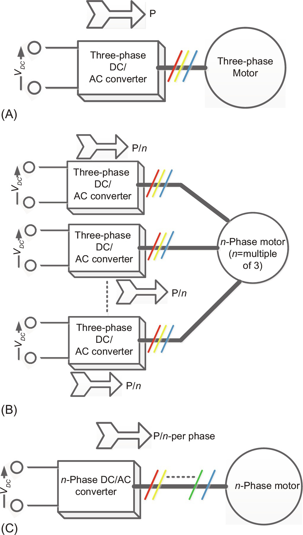
Solution of Fig. 15.1C, in contrast to the previous solution, works with a single inverter of n-phases supplying electric motor of n-phase. Each phase or leg now handles P/n power, and the circulating current is absent. The electric motor in this case is called symmetrical n-phase motor. This solution is also employed in high-power marine drive applications [6].
Reliability and fault tolerance are other driving forces leading to the development of multiphase system. Due to high phase number, fault tolerance is inherently guaranteed, which is of high importance in safety critical applications such as ship propulsion, more electric aircrafts, electric vehicles, and industrial setup where production loss is critical such as oil and gas plants and military. The multiphase motor drive guarantees continuous operation, however, with degraded performance under fault conditions. The higher the phase number, the better is the performance during faults. This make them highly attractive in applications mentioned above [7,8].
According to classical electric machine theory, the air-gap flux harmonic content improves and becomes close to sinusoidal with the increase in the number of phases. The improved flux density waveform leads to: (i) reduced rotor losses due to flux pulsation and eddy currents (this has importance for high-speed permanent magnet machines since the eddy current losses are very high at high speed in such kind of machines) and (ii) improved torque quality with reduced amplitude of torque pulsation that occurs at higher frequency (this is very important when machine is subjected to high distorted current, and limits are enforced on the maximum allowable torque pulsation).
Multiphase generators, specially five phases and more, have started to find a slot in the market due to their advantages over three-phase counterpart [9,10]. This multiphase system could be more suitable for direct drive wind energy, microturbines, and electric vehicle applications since the need for gears can be minimized. Multipulse rectifiers are employed, which have the ability to reduce the line current harmonic distortion and normally do not require any LC filters or power factor improvement devices. Multipulse DC can be obtained either by increasing the number of phases of the converter or by the use of phase-shifting transformer along with special secondary winding connections in the conventional six-pulse rectifiers. In drive application, the use of phase-shifting transformer provides an effective means to block common-mode voltages generated by the rectifier and inverter, which would otherwise appear on motor terminals, leading to a premature failure of machine winding insulation. Normally AC-DC converters are classified into power factor control rectifiers operated at high switching frequency and line-commutated rectifiers (uncontrolled or controlled) operated at power frequency or generated frequency. The multiphase line-commutated converter normally offers simple control, simple construction, and low cost but suffers from poor input power factor, low input current THD, and unidirectional current flow. The shortcoming of line-commutated rectifiers is overcome by the use of high-switching-frequency PWM rectifiers, voltage-source rectifiers, or current-source rectifiers, but the switch current and voltage limitation may restrict the use of PWM rectifiers in high-power applications.
Multiphase DC-AC voltage-source inverter is obtained from three-phase voltage-source inverter by adding extra legs (each leg has two switches in two-level inverter and a higher number of switches for multilevel inverter). The two switches of the same leg are complimentary in operation (i.e., when upper switch is on, the lower switch must be off and vice versa). The power switches can assume only two states, that is, on (called level 1) or off (called level 0). Hence, as such for n-phase inverter, there can be 2n number of switching states. Considering a three-phase inverter, the number of switching states are 8, and, for example, for a nine-phase inverter, the number of switching states are 29=512 [5]. It is seen that the number of switching states increases significantly with the increase in the number of phases or legs. Higher numbers of switching states offer flexibility in devising control techniques. Thus, multiphase inverter control has several degrees of flexibility in control. Multiphase inverter can be controlled using different PWM techniques such as carrier-based sinusoidal PWM, harmonic injection PWM, selective harmonic PWM, hybrid PWM, and space-vector PWM. Each method can produce different output magnitudes. Simple carrier-based PWM for multiphase inverters works exactly the same as for three-phase inverters. The maximum possible output phase-to-neutral voltage is 0.5 VDC, where VDC is DC-link voltage magnitude for multiphase inverter [1]. However, the output phase-to-neutral voltage magnitude varies for different phase numbers when using space-vector PWM. Nevertheless, the output phase-to-neutral voltage of multiphase inverters is less than that of a three-phase inverter. Multiphase inverter space vectors are transformed into multiple orthogonal planes, and control is implemented in order to regulate each plane vectors. In multiphase variable-speed drives (with distributed winding multiphase machine), torque is controlled only from one plane vector (d-q), and the rest of the plane vectors produce distortion and hence need to be minimized using PWM techniques. When concentrated winding multiphase machines are supplied using multiphase voltage-source inverters, all plane vectors are used to enhance the torque production. This is a unique feature of concentrated winding multiphase machine not available in three-phase machines. When implementing high-performance control such as vector control and direct torque control, higher control flexibility is available, and different solutions can be implemented.
Multiphase AC-AC converter more popularly known as multiphase matrix converter (MPMC) is also formulated by adding extra legs in three-phase matrix converter configuration. They are classified as direct matrix converters (DMC) and indirect matrix converters (IMC). Each converter leg has three bidirectional power switches each connected to one phase of the utility grid system, and at the output, load is connected. The input is fixed voltage and fixed frequency supply, while the output is of variable voltage and variable frequency. There are configurations where the number of input phases is three while the output phase are more than three and vice versa [4,5]. The multiphase matrix converter encompasses the advantages of three-phase matrix converters and multiphase systems. The major application areas are envisaged in multiphase wind energy system. A matrix converter can be seen as an array of m×n bidirectional power semiconductor switches that can transform m-phase fixed voltage and fixed frequency input to n-phase variable voltage and variable frequency output without intermediate DC conversion stage. The input side of a matrix converter is voltage fed, while the output side is current fed, and hence, an inductive filter is required at the output side, and a capacitive filter is used at the input side. As the load is itself of inductive nature, the requirement of output filter diminishes. The size of the input filter used in matrix converter is significantly smaller than an equivalent voltage-source inverter.
Considering an m×n matrix converter, the number of switching states is 2m×n. Large numbers of switching states are produced; however, not all of them are useful. Due to the nature of input (being voltage source) and output (being current source), the input should not short-circuited, and the output should not be open-circuited. As a consequence, only one switch in each leg conducts at one instant of time, and hence, a usable number of switching states are mn. In matrix converter, the output (sinusoidal) is formed from input (sinusoidal), and hence, output can assume any level depending upon the instantaneous value of the input. This makes the switching logic of matrix converter quite complex. The output voltage of a three-phase input and three-phase output matrix converter is 86.6% of the input voltage. The output-voltage magnitude reduces for higher phase number of outputs; for example, for a three-phase input and five-phase output matrix converter, it is 78.86% [11], and this value decreases further with increase in the output number of phases. The output voltage becomes higher than the input for m×n matrix converter for m>n; for example, for a five-phase input and three-phase output, it is 104.4%, and this value further increases as m is increased [4,12].
Multiphase matrix converters are constructed from bidirectional power switches that are realized in the same way as a three-phase matrix converter. The modulation strategies are complex and can be built upon the concept of three-phase matrix converter. However, significant challenges exist in obtaining proper modulation technique for a multiphase matrix converter. Some modulation strategies discussed in the literature are carrier-based PWM, space-vector PWM, and direct-duty-ratio-based PWM [13–19].
Multiphase matrix converters find its application in wind energy generation [20], power system [21,22], and ship propulsion [23]. When used in multiphase energy generation, usually the input side of the matrix converter is of higher phase, and the output side is three-phase connected to either utility grid or feeding isolated load. A 27-phase input and 3-phase output matrix converter of 100 MW power rating is presented in [24,25].
Present-day advancement in powering processors invariably uses multiphase buck converter topology because of higher output current and low-voltage requirement. Single-phase buck converter works well for low-voltage applications with currents up to 25 A. Higher filtering requirement and efficiency issue limits the use of single-phase topology in applications such as voltage regulator module (VRM). Interleaving as technically known reduces ripple currents at the input and output. A multiphase buck converter reduces considerably the i2R current power dissipation in the controlled switches and inductors. The distribution of current in various paths in a multiphase converter reduces the current magnitude through the switches, thereby reducing the switching losses. The output filter requirement decreases in a multiphase implementation due to the higher frequency of ripple current as a result of ripple current cancelation in the power stage for each phase. The single-phase implementation has much higher ripple content. Load transient performance is also better because of the reduction in energy stored in each output inductor. The lower the ripple current is, the less the perturbation will be. The input capacitors supply all the input current to the buck converter if the input wire to the converter is inductive. Improvement in multiphase topologies and their control strategies promise improved performance compared to the conventional multiphase buck converter.
This chapter is organized into five different sections covering the topologies, operation, and control of different types of multiphase power converters. Section 15.2 describes the types and classifications of different multiphase power converters. Section 15.3 is dedicated to AC-DC converters considering multiphase and multipulse output. Section 15.4 is devoted to DC-AC converters especially focusing on five-phase and seven-phase voltage-source inverter. Section 15.5 covers the description of multiphase AC-AC converters, and multiphase DC-DC converters are discussed in Section 15.6.
15.2 Types and Topologies of Multiphase Converters
The requirements for the current and voltage continue to increase with an increase in power level, and systems become more and more complex. The amount of current/voltage of power source to meet such requirements usually needs a combination of several power controllers to improve the thermal stress of the individual power components. The driving mechanism for this combination leaves one with two choices: single phase or multiphase.
Multiphase converters reduce the input and output current ripples by interleaving the two or more stages of power converters. By increasing the phase number, the output-voltage ripple and the input capacitor size can be curtailed without increasing the switching frequency of the power devices. Load dynamic performance is significantly improved during transients due to lower-output-voltage ripple and smaller output inductors. The low switching losses and driver circuit losses of power semiconductor devices at relatively low switching frequency and the reduced power losses due to equivalent series resistance (ESR) of the capacitors help achieve overall high efficiency of converters. For multioutput applications, multiphase converters may also provide the benefit of smaller input side capacitors.
Single-phase versus multiphase converters are as follows:
(1) Single-phase converters work well for low voltages and up to certain amount of current say about 25 A, but power dissipation and efficiency start to become an issue at higher currents. One suitable approach is to develop multiphase converters [26].
(2) The output filter requirements decrease in multiphase implementation due to the reduced current in the power stage for each phase. Compared with single-phase approach, the inductance and inductor size are drastically reduced because of lower average current and lower saturation current.
(3) Ripple current cancelation in the output filter stage results in a reduced ripple voltage across the output capacitor compared with single-phase approach. This is another reason why a multiphase converter is preferred.
(4) Load transient performance is improved due to the reduction of energy stored in each output inductor. The reduction in ripple voltage as a result of current cancelation contributes to minimal output-voltage overshoot and undershoots because many cycles will pass before the loop responds. The lower the ripple current is, the less the perturbation will be.
Like single-phase or three-phase converters, multiphase converters are classified as AC-DC, DC-AC, DC-DC, and AC-AC converters. Multiphase converters are simple extension of three-phase converters. As far as hardware is concerned, there is not much difference. However, the control complexity increases manyfold with the increase in the number of phases. There are further classifications in these converters. The classification of multiphase converters is shown in respective section.
15.2.1 Multiphase AC-DC Converters
A significant amount of work is done on developing novel topologies of multipulse AC-DC converters since they have huge potential applications for unidirectional and bidirectional power flow starting from six pulses to a large number of pulses. The major advantage of adopting a higher pulse number is the current ripple reduction.
The novel configurations in multiphase AC-DC converter were developed of unidirectional and bidirectional topologies with three or more number of phases. Classification of multiphase AC-DC converters is shown in Fig. 15.2, which is based on power flow, number of pulse used, isolated and nonisolated topologies, and various techniques used to improve AC current profile and output DC voltage waveform [27]. Based on the application and requirements, some systems require unidirectional power flow, and some require bidirectional power flow.
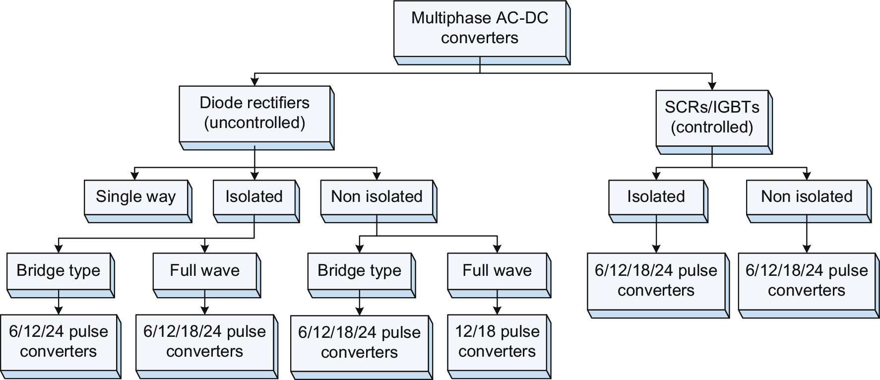
Unidirectional systems use diode rectifiers and transformer circuit configurations in isolated and nonisolated topologies. The unidirectional topologies have configurations of six pulses and its multiple. If the voltage difference is more between input and output, then isolated configuration is useful, and if the difference is less, nonisolated topologies are used. However, these are further classified as bridge and full-wave rectifiers. These types of full-wave multipulse converters (MPC) can also be further classified whether it uses double star or tapped polygon transformer secondary to create twelve phases to feed full-wave diode rectifiers. Both configurations have their own merits and demerits, but both MPC configurations show the same performance in terms of device and transformer utilization.
On the other hand, the bidirectional AC-DC converters have the power flow from AC mains to DC output or vice versa and normally use thyristors with phase angle control to obtain wide varying DC output voltages. These MPCs use multiple winding transformers to generate higher number of the phases. Like unidirectional, these MPCs are also divided as isolated and nonisolated. These are mainly used to feed DC motor drives and synchronous motor drives.
15.2.2 Multiphase DC-DC Converters
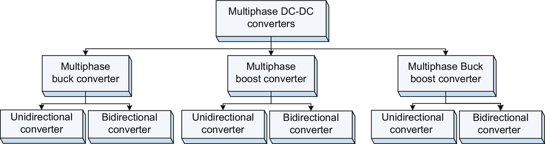
Multiphase topologies can be configured as a step-down (buck), step-up (boost), buck boost, and even forward converter. A multiphase DC/DC converter according to the present invention includes a plurality of DC/DC converters whose outputs are connected in common to supply electric power to a load and a load state detection portion that detects a state of the load connected to the plurality of DC/DC converters and outputs a detection result. Multiphase DC-DC converters classification is shown in Fig. 15.3.
15.2.3 Multiphase DC-AC Converters
Multiphase DC-AC converters are the main source of multiphase adjustable-speed drives. The major driving force behind the adoption of multiphase motor drive is due to the power segmentation in large number of converter legs. The power switching devices have limited voltage- and current-handling capabilities. Hence, when used in high-power application, series-and parallel combination of devices are required. This is cumbersome solution because of dynamic voltage sharing problem among the series-/parallel-connected power switching devices. Better solution is obtained when the power per phase or per leg is reduced by increasing the number of phases or number of legs, and this is termed as multiphase DC-AC inverters. Multiphase DC-AC inverters are simple in design as they are simple extension of three-phase DC-AC inverter. However, they offer large degree of switching redundancies and hence great flexibility in control. Although control becomes complex, the performance is improved manifold. Multiphase DC-AC inverters can be built in the same topologies as that of their three-phase counterparts and hence have the same calcifications and types. Multiphase AC-DC converters normally classified as shown in Fig. 15.4.

First version of multiphase inverter technology is five-phase VSI fed to star-connected five-phase load. Five-phase VSI configuration found application for five-phase induction machine and synchronous machine drives. Six-phase inverter configuration was built with two two-level standard three-phase VSIs, with two separate DC sources fed to dual three-phase induction motor. Seven-phase VSI fed to star-connected seven-phase load based on multiple space-vector modulation and seven-phase VSI configuration found applications for seven-phase permanent magnet synchronous and synchronous reluctance motor drives. Fig. 15.5 shows simple five-phase induction motor drive.
Multiphase inverters are also classified as cascaded H-bridge, diode clamped, and flying capacitor topologies. They can also be built in hybrid configuration. Multiphase impedance-source inverters (ZSI) and quasi impedance-source inverters (qZSI) are also reported in the literature [28]. ZSI and qZSI are special inverters that have the capability of boosting the source voltage and inverting DC to AC simultaneously. The boosting can be as high as 200%–300%. They are popular in solar PV applications since boosting and inversion is done in a single stage. Multiphase ZSI/qZSI is used to feed multiphase motor drives.
15.2.4 Multiphase AC-AC Converters
Multiphase AC-AC converters are generally classified as AC voltage controllers, matrix converters, and cycloconverters. Fig. 15.6 shows various topologies of multiphase AC-AC converters. AC voltage regulators are further classified as phase-controlled converters and fully controlled voltage converters.

Three-phase cycloconverters are of several types. For example, there are the 3-pulse cycloconverters, 6-pulse cycloconverters, and 12-pulse cycloconverters. Typically, the three-pulse converter is built with the three single, and the six-pulse converter is generally the combination of two three-pulse converters and so on. The 12-pulse converter is obtained by connecting two six-pulse configurations in series and appropriate transformer connections for the required phase shifted. Multiphase AC-AC converter classification is shown in Fig. 15.6. By using the knowledge of constructing a DC-modulated single-stage AC/AC converter, a multistage AC/AC converter can be easily obtained. Examples with complex structures are Luo converter, superlift Luo converter, and multistage cascaded boost converter. Using the same technique, one can construct DC-modulated multiphase AC/AC converters where they are classified as multiphase AC/AC buck, boost, and buck-boost converter.
Cycloconverters are broadly classified as naturally commutated and forced commutated. The later one is also known as matrix converter. Multiphase matrix converters are in study and are being studied in detail [4]. Fig. 15.7 shows some of the possible configurations of frequency changers. The one with a DC link is also commonly known as back-to-back (B2B) topology. Although B2B converter does the AC-AC conversion, it is sort of a paradigm to classify the topologies without the DC link under AC-AC converters. Also, the figure shows the possibility of research in the field of multiphase matrix converters.

15.3 Multiphase Multipulse AC-DC Converters
Solid-state AC-DC converters are widely used in a number of applications such as adjustable-speed drives (ASDs), high-voltage DC (HVDC) transmission, and electrochemical processes such as electroplating, telecommunication power supplies, battery charging, uninterruptible power supplies (UPS), high-capacity magnet power supplies, high-power induction heating equipment, aircraft converter systems, plasma power supplies, and converters for renewable energy conversion systems. These converters, which are also known as rectifiers, are generally fed from three-phase AC supply in power rating above few kilowatts. They exhibit the problems of power quality in terms of injected harmonics, resulting in poor power factor, AC voltage distortion, and rippled DC outputs. Because of these problems in AC-DC conversion, several standards and guidelines are laid down, which are to be referred by designers, manufacturers, and users. Therefore, various methods are used to mitigate these problems in AC-DC converters. Normally, filters are recommended in already existing installations, which may be passive, active, or hybrid types depending upon rating and economic considerations. These filters have been developed from small to large power ratings to reduce the power quality problems of AC-DC converters. However, in some cases, the ratings of these filters are close to the converter rating, which not only increases the cost but also increases the losses and component count, resulting in reduced reliability of the system. However, in future installations, it is preferred to modify the converter structure at design stage either using active or passive (magnetic) wave shaping of input currents or using multipulse AC-DC converters by using multiphase system or different connections of standard three-phase six-pulse AC-DC converters. At higher power level, generally, multiphase system is preferred. It reduces the ripples in the line current and load voltages drastically, and thus, EMI reduces, and the harmonic filter requirements also become very nominal.
15.3.1 Five Phase Uncontrolled Full Wave Bridge Rectifier
The circuit diagram of a simplified five-phase (ten pulses) uncontrolled rectifier consisting of 10 diodes (D1–D10) is shown in Fig. 15.8, where van, vbn, vcn, vdn, and ven are the supply phase voltages having peak value of Vm given by Eq (15.1):

van=Vmsin(ωt)vbn=Vmsin(ωt−2π/5)vcn=Vmsin(ωt−4π/5)vdn=Vmsin(ωt−6π/5)van=Vmsin(ωt−8π/5)

The diodes are assumed ideal and are numbered according to their conduction sequence 1,2- ,3- 3,4- 4,5- 5,6- 6,7- 7,8- 8,9- 9,1.
The line voltages for adjacent phases will be different from that of nonadjacent phases. The line voltages for adjacent and nonadjacent phases can be obtained from the respective phasor diagrams shown in Figs. 15.9 and 15.10, respectively, as follows:

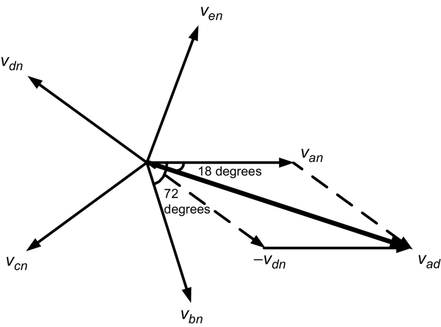
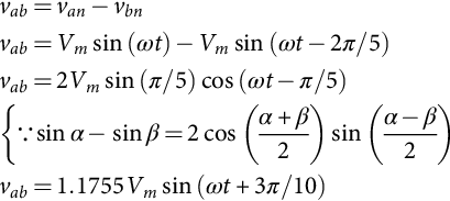
For adjacent phases,
vab=van−vbnvab=Vmsin(ωt)−Vmsin(ωt−2π/5)vab=2Vmsin(π/5)cos(ωt−π/5){∵sinα−sinβ=2cos(α+β2)sin(α−β2)vab=1.1755Vmsin(ωt+3π/10)
For nonadjacent phases,
vad=van−vdn=Vmsin(ωt)−Vmsin(ωt−6π/5)=2Vmsin(3π/5)cos(ωt−6π/10)vad=1.9021Vmsin(ωt−π/10)

Fig. 15.11A shows the waveforms of the maximum and minimum value of phase voltage in different intervals. The maximum phase voltage Vpn and minimum phase voltage Vqn described by Eq (15.4) will appear at the output terminals p and q. Both the diodes in the same leg never conduct simultaneously, which avoids direct short circuit in the leg. In the upper leg, the diodes (odd numbered) having its anode connected with phase voltage of highest value among phases will conduct. Similarly, in the bottom leg, the diodes (even numbered) having its cathode connected with lowest phase voltage will conduct at any instant of time:
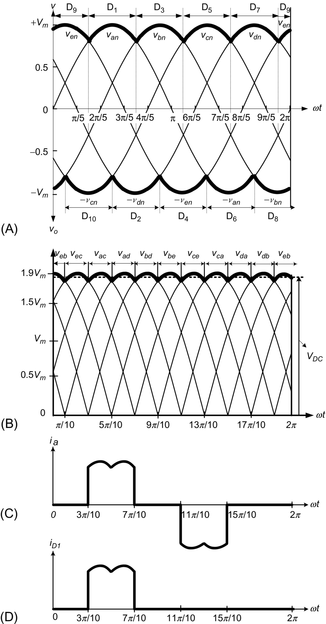
Vpn=max(van,vbn,vcn,vdn,ven)Vqn=min(van,vbn,vcn,vdn,ven)

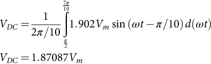
The output-voltage waveform shown in Fig. 15.11B is a 10-pulse waveform appearing across the load. For a purely resistive load, the waveform of the line current ia shown in Fig. 15.11C has two humps per half cycle of the supply frequency. The other four line currents, ib, ic, id, and ie, have the same waveform as ia but lag from ia by 2π/5, 4π/5, 6π/5, and 8π/5 radians, respectively. The average and rms value of output voltage at load can be calculated as
VDC=12π/107π10∫π21.902Vmsin(ωt−π/10)d(ωt)VDC=1.87087Vm
Vrms=√12π/107π10∫π2[1.902Vmsin(ωt−π/10)]2d(ωt)Vrms=1.87107Vm

For a resistive load, the harmonics of the output voltage can be found by using Fourier series analysis. To find the Fourier coefficients, we integrate vbe from −π/10 to +π/10. Considering the half-wave symmetry, the Fourier coefficients will be calculated as follows:
bn=0
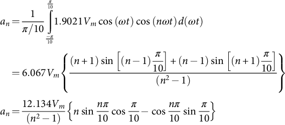
an=1π/10π10∫−π101.9021Vmcos(ωt)cos(nωt)d(ωt)=6.067Vm{(n+1)sin[(n−1)π10]+(n−1)sin[(n+1)π10](n2−1)}an=12.134Vm(n2−1){nsinnπ10cosπ10−cosnπ10sinπ10}
If the frequency of the source voltage is f, the output voltage has harmonics at 10f, 20f, 30f …etc. Eq. (15.8) is simplified as
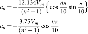
an=−12.134Vm(n2−1){cosnπ10sinπ10}an=−3.75Vm(n2−1)cosnπ10
The DC component is found by putting n=0 in Eq. (15.9), and its value is
VDC=a02=1.87Vm
This is the same value as calculated in Eq. (15.5). The Fourier series of the load voltage can be written as
vL(t)=a02+∞∑n=10,20,⋯ancos(nωt)

After substituting the values of the coefficients, we obtain
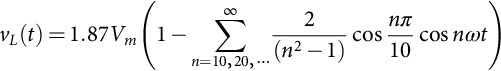
vL(t)=1.87Vm(1−∞∑n=10,20,⋯2(n2−1)cosnπ10cosnωt)
vL(t)=1.87Vm(1+299cos10ωt−2399cos20ωt+⋯)
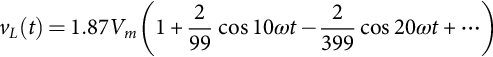
Fig. 15.12 shows the load voltage harmonics profile. Since each diode conducts one fifth of the time, the average diode current is given by Eq. (15.14).

ID,avg.=12π[7π10∫3π10IDCd(ωt)]=0.2IDC
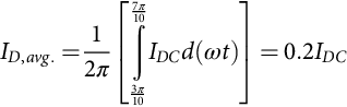
Eq. (15.14) indicates that a five-phase rectifier will have switches with lower ratings as compared with the three-phase counterpart, provided that both are feeding the same load as average value of switch current in three-phase system is 33.33% and in this case it is 20% [9,10]. The input phase current can be expressed as
is=∞∑n=1,3,5....4IDCnπsinnπ5sin(nωt)

The fundamental component of input current is
is1=0.7484IDCsin(ωt)
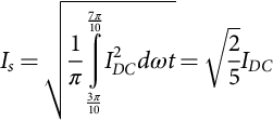
The rms value of the fundamental component of input current is
Is=√1π7π10∫3π10I2DCdωt=√25IDC
Problem 15.1
A five-phase bridge rectifier delivers 60 A current at a voltage of 317.5 V to a purely resistive load. If the frequency of the source is 60 Hz, determine the following:
(a) Efficiency of rectification
(b) Form factor
(c) Ripple factor
(d) Peak inverse voltage (PIV) of each diode
(e) Peak current through a diode
Solution
Since VDC=1.87087Vm and Vrms=1.87101Vm and also IDC=VDC/R and Irms=Vrms/R,
(a) Efficiency of rectification η=PacPDC=Vrms2RVDC2R=(1.87107)2(1.87087)2=99.97%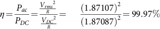
(b) Form factor FF=VrmsVDC=1.87107187087=100.011%![]()
(c) Ripple factor RF=√FF2−1=√(1.00011)2−1=1.483%![]()
(d) Peak inverse voltage of each diode=1.902Vm
Also, since VDC=1.87087 Vm and peak value of phase voltage, Vm=VDC1.87087=317.51.87087=169.70V![]()
Hence, PIV=1.902×169.70=322.78V![]()
(e) The average DC current through each diode is
IDC(Diode)=IDC5=605=12A

Also, IDC(Diode)=4ππ10∫0Imcosωtdωt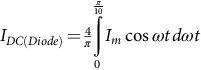
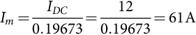
IDC=0.19673Im
Im=IDC0.19673=120.19673=61A
15.3.2 Five-Phase Controlled Full Wave Bridge Rectifier
Whenever a diode is in forward-biased condition, it conducts, but a thyristor (or controlled switch) requires a triggering signal for its conduction. If all the diodes of a 10-pulse full-wave uncontrolled converter are replaced by controlled switches (thyristors), it becomes a controlled converter. Fig. 15.13 shows the basic power circuit of a fully controlled 10-pulse 5-phase AC-DC converter. In this case, the thyristors are switched at an interval of 36 degrees sequentially as shown in Table 15.1. When T1 and T2 are conducting van and vbn voltages with respect to neutral appear at the load, that is, vad=van−vdn, which is the line voltage VL (vad=1.9021Vmsin(ωt−π/10)![]() ). At ωt=π/2+α, T1 is commutated, as on this instant of time vbn>van, and the load current is transferred from T1 to T3. There are 10 voltage pulses, and the instantaneous output voltage may become negative for an RL load, but the Vdc will always have positive value, except for an active (RLE) load. It should be noted that the line voltage corresponding to the nonadjacent phase voltages is only appearing across the load. AC voltages applied to the rectifier is given by Eq. (15.1).
). At ωt=π/2+α, T1 is commutated, as on this instant of time vbn>van, and the load current is transferred from T1 to T3. There are 10 voltage pulses, and the instantaneous output voltage may become negative for an RL load, but the Vdc will always have positive value, except for an active (RLE) load. It should be noted that the line voltage corresponding to the nonadjacent phase voltages is only appearing across the load. AC voltages applied to the rectifier is given by Eq. (15.1).

Table 15.1
Thyristor firing instants and output voltage across the load
| Time interval | Thyristor fired | Conducting thyristor | Output voltages across load |
| [π/10+α, 3π/10+α] | T10 | T9 and T10 | vo=vec=1.902Vmsin(ωt+3π/10) |
| [3π/10+α, 5π/10+α] | T1 | T10 and T1 | vo=vac=1.902Vmsin(ωt+π/10) |
| [5π/10+α, 7π/10+α] | T2 | T1 and T2 | vo=vad=1.902Vmsin(ωt−π/10) |
| [7π/10+α, 9π/10+α] | T3 | T2 and T3 | vo=vbd=1.902Vmsin(ωt−3π/10) |
| [9π/10+α, 1π/10+α] | T4 | T3 and T4 | vo=vbe=1.902Vmsin(ωt−π/2) |
| [11π/10+α, 13π/10+α] | T5 | T4 and T5 | vo=vce=1.902Vmsin(ωt−7π/10) |
| [13π/10+α, 15π/10+α] | T6 | T5 and T6 | vo=vca=1.902Vmsin(ωt−9π/10) |
| [15π/10+α, 17π/10+α] | T7 | T6 and T7 | vo=vda=1.902Vmsin(ωt+9π/10) |
| [17π/10+α, 19π/10+α] | T8 | T7 and T8 | vo=vdb=1.902Vmsin(ωt+7π/10) |
| [19π/10+α, 21π/10+α] | T9 | T8 and T9 | vo=veb=1.902Vmsin(ωt+5π/10) |

The delay angle reference is taken from the point the thyristor would begin to conduct if it were a diode. Thus, the delay angle is an interval from the thyristor being forward-biased and till the gate signal is applied. The corresponding waveforms are shown in Fig. 15.14A–H [9,10]. Since each voltage pulse corresponds to the line voltage and it appears for 1/10th period of the cycle 2π/10, the average output voltage corresponding to vad shown in Table (15.1) is given by

VDC=12π107π10+α∫5π10+α1.902Vmsin(ωt−π/10)d(ωt)VDC=5×1.902Vmπ[−cos(ωt−π/10)]7π10+α5π10+αVDC=1.87Vmcosα

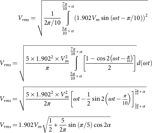
The rms output voltage is
Vrms=√12π/107π10+α∫5π10+α(1.902Vmsin(ωt−π/10))2Vrms=√5×1.9022×V2mπ7π10+α∫5π10+α[1−cos2(ωt−π10)2]d(ωt)Vrms=√5×1.9022×V2m2π[ωt−12sin2(ωt−π10)]7π10+α5π10+αVrms=1.902Vm√12+52πsin(π/5)cos2α
It is evident from Fig. 15.14D that the instantaneous output voltage is continuous for α<π/5; therefore, for any passive load, the load current will be continuous. For 3π/10<α>π/5, the continuity of load current depends on the phase angle of load (φ) and discontinuous for purely resistive load (φ=0). For α>3π/10, the load current will be always discontinuous for the passive load (Vdc>0), whereas for active load (RLE), there will be fourth-quadrant operation (Vdc<0 and Idc>0).
Fig. 15.14E shows the input phase current, which is a quasisquare wave. Since the instantaneous value of load current is assumed to be constant, so the phase current will be +IDC in the interval (3π/10+α and 7π/10+α) and −IDC in the interval (13π/10+α and 17π/10+α). Also, each phase currents will be displaced from each other by 2π/5, irrespective of thyristor firing angles. The input phase current ia can be expressed in Fourier series as
ia=IDC+∞∑n=1,2,3,…(ancosnωt+bnsinnωt)ia=IDC+∞∑n=1,2,3,…√2Insin(nωt+φn)

where In is the rms value of nth harmonic component of the input current and is given by
In=1√2(a2n+b2n)12

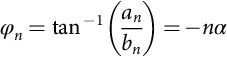
The φn is the nth harmonic phase shift and is given by
φn=tan−1(anbn)
Also, due to the symmetry of waveform,
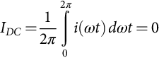
IDC=12π2π∫0i(ωt)dωt=0
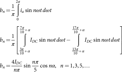
an=1π2π∫0iacosnωtdωtan=1π[7π10+α∫3π10+αIDCcosnωtdωt−17π10+α∫13π10+αIDCcosnωtdωt]an=−4IDCnπsinnπ5sinnα,n=1,3,5,…
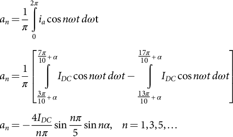
Similarly,
bn=1π2π∫0iasinnωtdωtbn=1π[7π10+α∫3π10+αIDCsinnωtdωt−17π10+α∫13π10+αIDCsinnωtdωt]bn=4IDCnπsinnπ5cosnα,n=1,3,5,…
Therefore, the rms value of nth harmonics current will be given by
In=1√2(a2n+b2n)12=2√2nπIDCsinnπ5

and
φn=tan−1(anbn)=−nα
n=1 will give the rms value of fundamental component of the input current:
I1=2√2πIDCsinπ5=0.529IDC

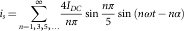
Hence, the input current can be given by
is=∞∑n=1,3,5,…4IDCnπsinnπ5sin(nωt−nα)
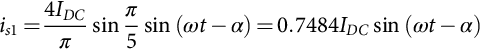
The fundamental input current, (substituting, n=1), is
is1=4IDCπsinπ5sin(ωt−α)=0.7484IDCsin(ωt−α)
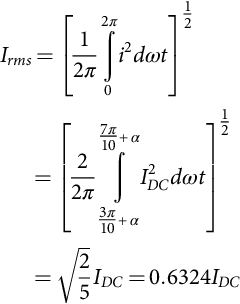
The rms value of the input current can be calculated as
Irms=[12π2π∫0i2dωt]12=[22π7π10+α∫3π10+αI2DCdωt]12=√25IDC=0.6324IDC
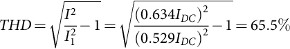
The total harmonic distortion (THD) is given by
THD=√I2I21−1=√(0.634IDC)2(0.529IDC)2−1=65.5%
Displacement factor
DF=cos(φ1)=cos(−α)=cosα
Power factor
PF=cosα√1+THD2=I1Icosα=0.529IDC0.634IDCcosα=0.8365cosα

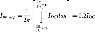
The load current is constant as the load is considered highly inductive; from Fig. 15.14F, it is clear that each switch operates for 2π/5 period of time in one cycle; accordingly, the switch average current can be calculated as
Isw_avg.=12π[7π10+α∫3π10+αIDCdωt]=0.2IDC
When calculated, the switch current is only 20% of DC-link current [10]. The harmonic factor (HFn) is defined as the normalized harmonic current of the supply with respect to the fundamental component (In/I1) and is calculated using Eq. (6.36):
HFn=√(InI)2−1

Problem 15.2
A five-phase full-wave bridge-controlled rectifier has an AC input of 120 V rms at 60 Hz and 100 Ω load resistor. The delay angle is α=π/12 radians. Determine the following:
(a) Average current in the load
(b) Power absorbed by the load
(c) Efficiency of the rectifier
(d) The expression for the input current
(e) THD
(f) Power factor of the rectifier
(g) Form factor and ripple factor
Solution
(a) Average load voltage VDC=1.87Vmcosα=1.87×√2×120×cos(π/12)=306.53V![]()
Average load current IDC=VDCR=306.53100=3.06A![]()
(b) Power absorbed by the load PDC=VDC×IDC=306.53×3.06=938W![]()
(c) The rms value of the output voltage Vrms=1.902Vm√12+52πsin(π5)cos2α![]()
Vrms=1.902×120√2√12+52πsin(π5)cos(2×π12)
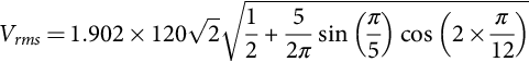
Vrms=307.08V
and Irms=VrmsR=307.08100=3.071A![]()
Therefore, efficiency η=PDCPac=VDCIDCVrmsIrms=306.53×3.06307.08×3.071=99.46%![]()
(d) The expression for the input current is=∞∑n=1,3,5,…4IDCnπsinnπ5sin(nωt−nα)
is=∞∑n=1,3,5,…3.9nsinnπ5sin(nωt−nπ/12)

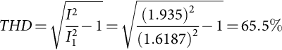
(e) The rms value of the input current I=√25IDC=√25×3.06=1.935A![]()
The rms value of fundamental component of the input current
I1=2√2πsinπ5IDC=0.529×3.06=1.6187

THD=√I2I21−1=√(1.935)2(1.6187)2−1=65.5%
(f) The power factor PF=cosα√1+THD2=cos(π/15)√1+(0.655)2=0.818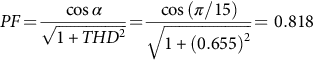
(g) Form factor FF=VrmsVDC=307.08306.53=1.0018=100.18%![]()
Ripple factor RF=√FF2−1=√(1.0018)2−1=0.06=6%![]()
15.3.3 Multipulse Rectifiers
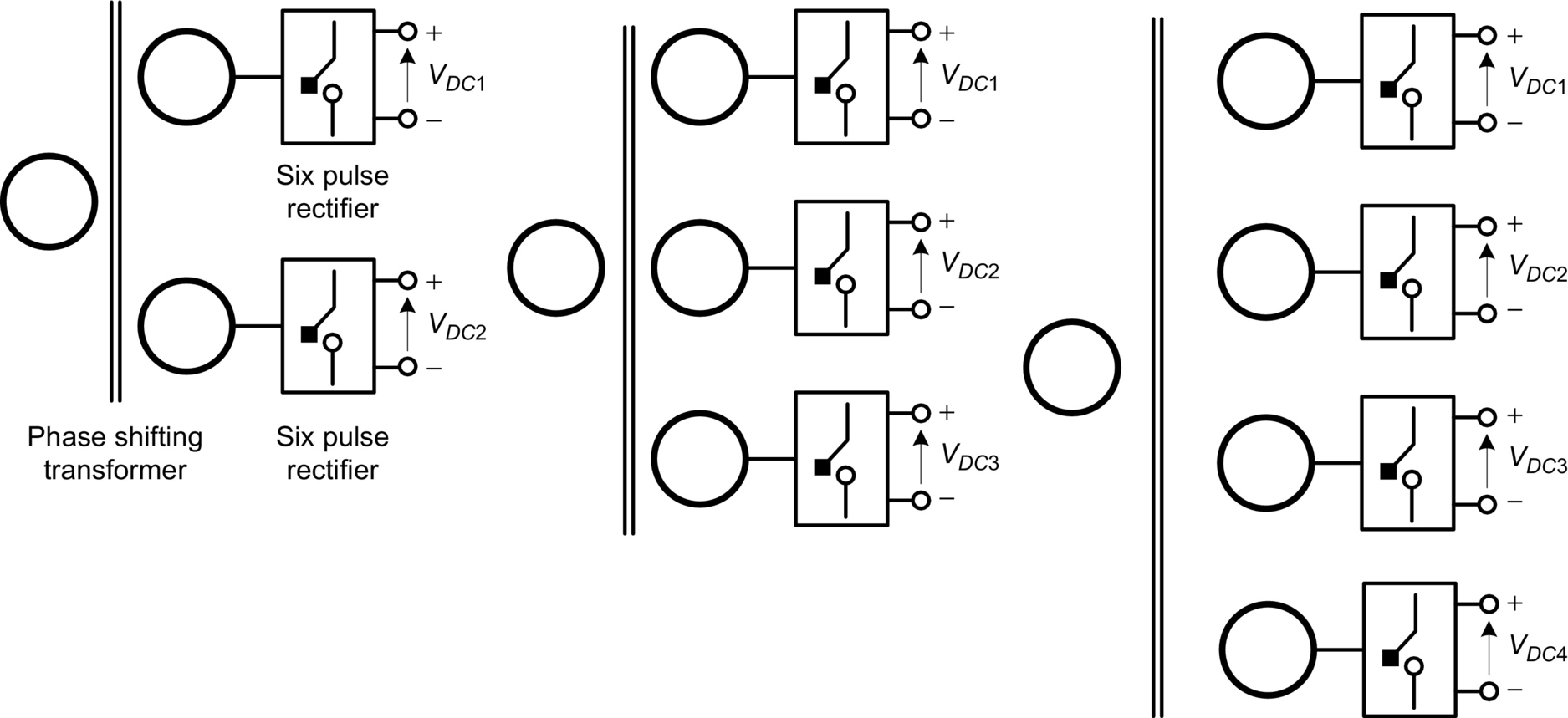
The multipulse uncontrolled rectifiers are suitable for VSI-fed drives, while the controlled rectifiers are employed for CSI drives. As the number of pulses per cycle increases, the output waveform gets improved. There are identical multipulse rectifiers connected in either parallel, series, or separate modes to achieve higher pulses in the output. Fig. 15.15 shows general layout of 12-, 18-, and 24-pulse rectifier circuits [29,30]. If we employ 10-pulse rectifiers, then we can obtain 20, 30, and 40 pulses in the output.
15.3.3.1 12-Pulse Series Type Controlled Rectifier
Two six-pulse controlled rectifiers are powered by a phase-shifting transformer with two secondary windings in delta and star connections. Therefore, the phase angle between both secondary windings shifts 30 degrees each. In this case with 12 pulses per cycle, the quality of output-voltage waveform would definitely be improved with low ripple content [29].
Fig. 15.15 shows circuit configuration of a 12-pulse series-type controlled rectifier. A three-phase transformer with two secondary and one delta-connected primary feeds the two identical six-pulse controlled rectifiers. The upper three-phase bridge is fed from Y-connected secondary winding while lower with Δ-connected secondary winding. Therefore, this arrangement will result in the phase angle shifts between both secondary windings by 30 degrees. The outputs of the two six-pulse rectifiers are connected in series, and the conduction period of the line current for each converter is 120 degrees.
Consider an idealized 12-pulse rectifier where the line inductance Ls and the total leakage inductance Llk of the transformer are assumed to be zero and the magnitude of the current is constant (ripple-free) [29]. In practical case, the ripple in the DC current will be relatively low due to the series connection of the two six-pulse rectifiers, where the leakage inductances of the secondary windings can be considered in series.
For the purpose of eliminating the dominate lower-order harmonics in the line current ia, the line-to-line voltage va1b1 of the Y-connected secondary winding (N2 turns) is in phase with the primary winding (N1 turns) voltage vab, while the Δ-connected secondary winding (N3 turns) voltage va2b2 leads vab by [29]:
δ=∠va2b2−∠vab=30degrees
For the sake of simplicity, let N1=N,N2=N/2andN3=√3/2N![]() (i.e., N1-N2-N3=1:0.5:0.866).
(i.e., N1-N2-N3=1:0.5:0.866).
Therefore, the rms line-to-line voltage of each secondary winding will become
Va1b1=Va2b2=Vab/2
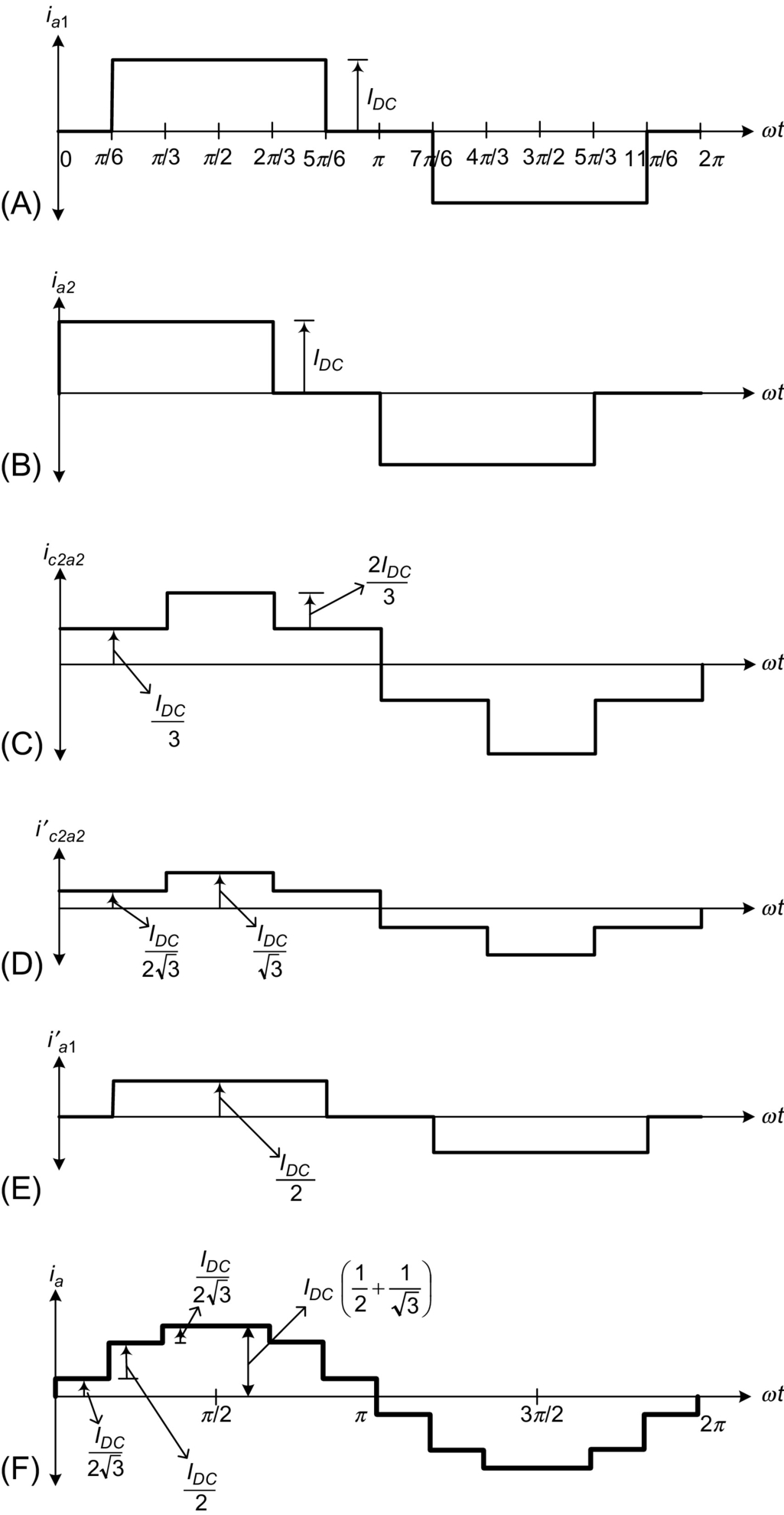
Since the two rectifiers are series-connected, net output, or load, voltage Vdc=Vdc1+Vdc2 ; since the waveforms of Vdc1 and Vdc2 are phase shifted from each other by 30 degrees , therefore, the waveform of output voltage Vdc consists of 12 pulses per cycle of supply voltage. The current waveforms are illustrated in Fig. 15.16, where ia1 and ic2a2 are the phase currents of secondary Y and Δ windings, respectively, and i′a1 and i′c2a2 are the currents referred from secondary side to the primary side. The waveforms of reflected current to primary side of secondary Y-connected winding i′a1 will be identical to that of ia1 except that the magnitude is changed in ratio of the number of turns of the two windings. However, when ia2 is referred to the primary side, the reflected waveform does not keep the same waveform and magnitude. This is due to phase displacements of the harmonic current when they are referred from Δ-Y windings. This phase displacement is advantageous as it will lead to the cancelation of low-order predominant fifth and seventh harmonics from the currents of transformer primary winding and does not appear in the line current, which is given by Eq. (15.39):
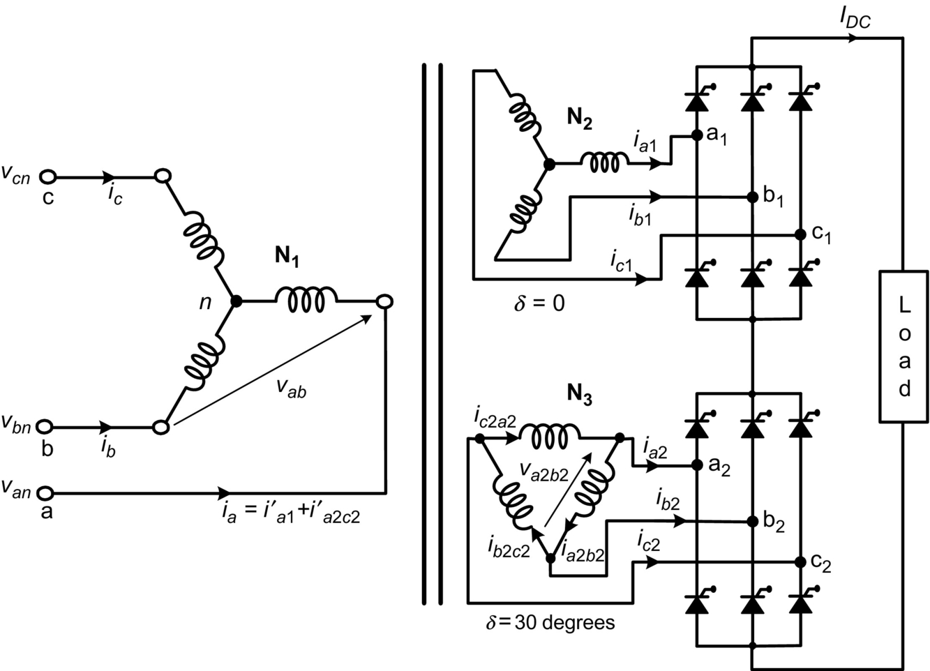
ia=i'a1+i'a2
The secondary (Y-connected) line current ia1 can be expressed by Eq. (15.40):
ia1=2√3πIdc[sinωt−15sin5ωt−17sin7ωt+111sin11ωt+113sin13ωt−117sin17ωt−119sin19ωt+…]

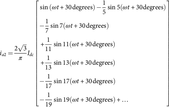
Since the waveform of current ia1 is of half-wave symmetry, it does not contain any even-order harmonics. Current ia does not contain any triple harmonics either due to the consideration of balanced three-phase system. The line current in Δ-connected secondary winding such as ia2 leads ia1 by 30 degrees, and the Fourier expression of current ia2 is given by Eq. (15.41):
ia2=2√3πIdc[sin(ωt+30degrees)−15sin5(ωt+30degrees)−17sin7(ωt+30degrees)+111sin11(ωt+30degrees)+113sin13(ωt+30degrees)−117sin17(ωt+30degrees)−119sin19(ωt+30degrees)+…]
Similar equations for ib2 and ic2 can be obtained. The current i′a1, which is identical to ia1 in wave shape, can be expressed in Fourier series by Eq. (15.42):
i'a1=√3πIdc(sinωt−15sin5ωt−17sin7ωt+111sin11ωt+113sin13ωt…)

The phase currents in the Δ-connected secondary windings ia2b2, ib2c2, and ic2a2 can be obtained from its line currents using the transformation given in Eq. (15.43):
[ia2b2ib2c2ic2a2]=13[−1100−1110−1][ia2ib2ic2]

The phase currents in the Δ-connected secondary winding ia2b2, ib2c2, and ic2a2 have a stepped waveform, each step being of 60 degrees in width whereas Id/3 and 2Id/3 the heights. The expression for phase current in the Δ-connected secondary winding can be written as Eq. (15.44).
ic2a2=2π√3Idc[sin(ωt+30degrees)−15sin5(ωt+30degrees)−17sin7(ωt+30degrees)+111sin11(ωt+30degrees)+⋯−sin(ωt+150degrees)+15sin5(ωt+150degrees)+17sin7(ωt+150degrees)−111sin11(ωt+150degrees)⋯]

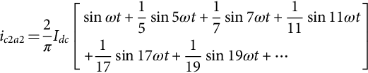
On simplification of Eq. (15.44), we have
ic2a2=2πIdc[sinωt+15sin5ωt+17sin7ωt+111sin11ωt+117sin17ωt+119sin19ωt+⋯]
Similarly, the expressions for the currents ia2b2 and ib2c2 can be obtained. The corresponding reflected current to the primary side can be obtained from Eq. (15.45); by multiplying with turn ratio (N3:N1=√3:2![]() ), we can obtain Eq. (15.46) [31]:
), we can obtain Eq. (15.46) [31]:
i'c2a2=√3πIdc[sinωt+15sin5ωt+17sin7ωt+111sin11ωt+113sin13ωt+117sin17ωt+119sin19ωt+123sin23ωt+125sin25ωt+⋯]
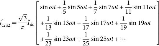
Therefore, the line current ia=i'a1+i'c2a2![]() can be written as given in Eq. (15.47):
can be written as given in Eq. (15.47):
ia=2√3πIdc[sinωt+111sin11ωt+113sin13ωt+123sin23ωt+125sin25ωt+⋯]
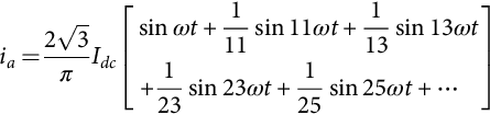
Different current waveforms are shown in Fig. 15.17. It is evident from Eq. (15.47) that the two dominant harmonics, 5th and 7th, are absent along with 17th and 19th, which improves the THD of this type of converter configuration drastically.
15.3.3.2 Pulse Parallel-Type Controlled Rectifier
In this case, the outputs of the two six-pulse rectifiers are connected in parallel. Fig. 15.18 shows circuit configuration of a 12-pulse parallel-type controlled rectifier. The circuit in the figure simply uses an isolation transformer with a Δ-connected primary, a Y-connected secondary, and a second Δ-connected secondary to obtain 30 degrees (electrical degrees) phase shift. Since the instantaneous outputs of the two rectifiers are not equal, an interphase reactor is necessary to support the difference in instantaneous rectifier output voltages and permit each rectifier to operate independently [29]. The line current in primary winding of the transformer is the sum of reflected currents from the two secondary windings, and it becomes stepped due to 30 degrees phase shift in two secondary currents as discussed in Section 15.3.3.1. Therefore, the harmonics and requirement of filter circuit parameters are reduced. Theoretically, input current harmonics for rectifier circuit is a function of pulse number and can be expressed as

H=(Np±1)
where N=1, 2, 3… and p is pulse number.
For example, in a three-phase six-pulse rectifier, the input current will have harmonic components at 5, 7, 11, 13, 17, 19, 23, 25, 29, 31, etc. multiples of the fundamental frequency. For the 12-pulse system shown in Fig. 15.16, the input current will have theoretical harmonic components at 11, 13, 23, 25, 35, 37, etc. multiples of the fundamental frequency as derived and discussed in Section 15.3.3.1. Since the magnitude of each harmonic is proportional to the reciprocal of the harmonic order, the 12-pulse system naturally has a lower harmonic distortion in input current.
The problem with the parallel connection of the rectifiers is that the two rectifiers must share exactly equal current to achieve the desired reduction in harmonics. This would be achieved if output voltages of both secondary windings matches exactly. Because of the differences in the transformer secondary impedances and open-circuit output voltages, this can be practically accomplished for a given fixed load (typically rated load), but not for loads varying over a range. This is the main problem of the parallel 12-pulse configuration connection. Whereas in the case of series connection of two rectifiers, the problems associated with current sharing are avoided, and an interphase reactor is not required. Parallel connections are normally preferred for applications where high current ratings rather than harmonics are the issue [32]. Generally, series connection of rectifiers is much simpler to implement than the parallel connection.
15.3.4 Single-Way Multiphase Systems Topologies
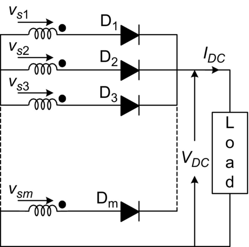
The structure of single-way, m-phase rectifier is shown in Fig. 15.19. In single-way structures, only one diode conducts for single stage, and the remaining diodes are blocked. Due to this, single-way structures are more convenient while increasing the number of phases. In an m-phase, the diodes used in the rectifier circuits are divided into a number of groups in star connection. Each group will have three diodes, that is, for a six-diode rectifier, there will be two groups, and for a 12-diode rectifier, there will be four groups [31]. In a normal connection, the star points will be connected together. But in this circuit, each group will have its all secondary windings, and instead of a direct connection, the star points will be connected through an interphase transformer. The common neutral point serves as the negative terminal of the DC output circuit.
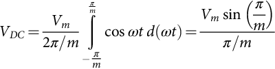
For single-way topologies, the number of output pulses is equal to the number of phases, that is, p=m, and the number of diodes are equal to m. Each diode is conducting for 2π/m electric radians. Fig. 15.19 shows few pulses of output-voltage waveform for m-phase half-wave uncontrolled rectifier. In general, for an m-phase system, the average and rms value of the output voltage is expressed by Eqs. (15.49) and (15.50), respectively:
VDC=Vm2π/mπm∫−πmcosωtd(ωt)=Vmsin(πm)π/m
rms voltage Vrms=√12π/mπm∫−πm(Vmcosωtdωt)2
Vrms=Vm√12[1+sin(2πm)2πm]

The form factor and ripple factors are expressed by Eqs. (15.51) and (15.52), respectively. From these equations, it is evident that ifm→∞⇒FF→1andRF→0![]() ,
,
FF=VrmsVDC=√12[1+sin(2πm)2πm]sin(πm)πm
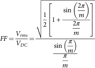
RF=√1−(FF)2
which implies that by increasing the number of phases in a multiphase, single-way rectifier, the output voltage is improved, that is, it becomes smoother. By connecting to a conventional three-phase mains distribution, it is possible to increase the number of “phases” by using transformers with m separated secondary coils. The secondary coils can be connected in a large number of ways. Also, by increasing the number of phases (as stated before, in single-way topologies, m=p), the ripple frequency increases, and its amplitude decreases. This fact simplifies the filter design to reduce the ripple in the load [31,32]. The output waveform for m-phase half-wave diode rectifier is shown in Fig. 15.20. For highly inductive load, the output DC current may be considered as constant (IDC).

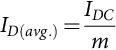
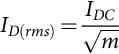
The diode average current, rms current, and form factor can be obtained by Eqs. (15.53)–(15.55):
ID(avg.)=IDCm
ID(rms)=IDC√m
Kf=ID(rms)ID(avg)=√m

The values for VDC and some of the parameters have been calculated for m=6, m=12, and m=24 and are reported in Fig. 15.21. It is clear from the figure (A)–(C) that the frequency of the ripple on the output is p times the mains frequency. As can be seen, passing from 6 to 12 pulses, one gets a 3.5% improvement in the rectified voltage, while passing from 12 to 24 pulses this improvement is less than 1%.

In practice, for single-way connections, the maximum number of pulses is normally limited to 12 because of the growing complexity of the connections of the transformer's secondary windings. Higher number of pulses can be obtained by using the combination of bridge structures. The best transformer utilization factor (TUF) that can be achieved with a single-way connection is 0.79, while with a bridge configuration it is possible to reach higher values, up to 0.955.
15.3.5 Six-Phase AC to DC Converters
Six-phase half-wave rectifiers generally have two configurations, namely, six phase with a neutral line circuit and double antistar with a balance-choke circuit.
15.3.5.1 Six-Phase Half Wave With a Neutral Line Circuit
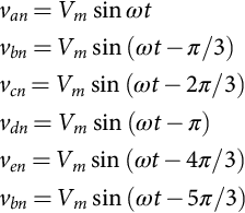
The power supply of a six-phase balanced voltage source is given by Eq. (15.56), and the waveform is shown in Fig. 15.22; in this case, each phase is shifted by 60 degrees:
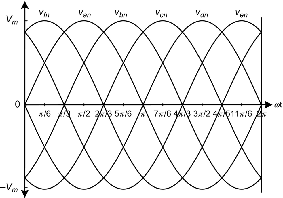
van=Vmsinωtvbn=Vmsin(ωt−π/3)vcn=Vmsin(ωt−2π/3)vdn=Vmsin(ωt−π)ven=Vmsin(ωt−4π/3)vbn=Vmsin(ωt−5π/3)
The six-phase half-wave rectifiers are shown in Fig. 15.23. The first circuit is called a Y-Y circuit, and the second circuit is called a Δ/Y circuit. Each diode conducts for 60 degrees in a cycle.

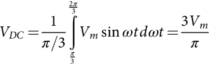
VDC=1π/32π3∫π3Vmsinωtdωt=3Vmπ
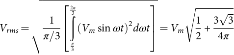
Vrms=√1π/3[2π3∫π3(Vmsinωt)2dωt]=Vm√12+3√34π
FF=VrmsVdc=1.0008
RF=√1.00082−12=0.04
PF=0.55
15.3.5.2 Six-Phase Double-Bridge Full-Wave Uncontrolled Rectifiers
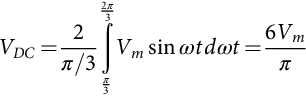
Two circuits of the six-phase bridge full-wave diode rectifiers are shown in Fig. 15.24 and are called as a six-phase bridge circuit and hexagon bridge circuit [31]. In this case, each diode conducts for 60 degrees in a cycle. The average output voltage is given by Eq. (15.62):
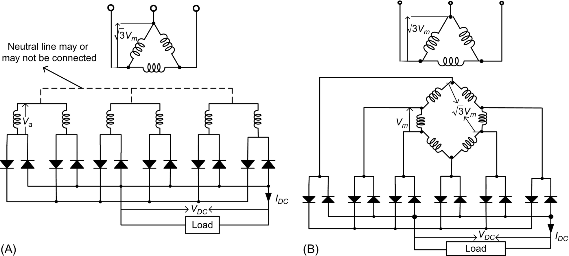
VDC=2π/32π3∫π3Vmsinωtdωt=6Vmπ
15.3.5.3 Six-Phase Half-Wave Controlled Rectifiers
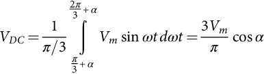
The six-phase half-wave controlled rectifiers are shown in Fig. 15.25 [31]. Each thyristor conducts for π/3 radians in a cycle. The firing angle α=ωt−π/3 in the range of 0–2π/3. The average output voltage is

VDC=1π/32π3+α∫π3+αVmsinωtdωt=3Vmπcosα
Vrms=√1π/3[2π3+α∫π3+α(Vmsinωt)2dωt]=Vm√12+3√34πcosα

FF=VrmsVdc=1.0008
RF=√1.00082−12=0.042
PF=0.956
From Eq. (15.63), it is clear that the output voltage can have positive (α<π/2) and negative (α>π/2) values. When α<π/2, the output current is (IDC=VDC/R), and when the firing angle α is >π/2, the output voltage can have negative values, but the output current can only have positive values.
15.4 Multiphase DC-AC Converters
15.4.1 Modeling and Control of a Five-Phase Voltage Source Inverter
This section is devoted to the development of a comprehensive model of a five-phase voltage-source inverter based on space-vector theory [32,33]. Proper modeling of voltage-source inverters is important in devising appropriate control algorithm. The complete model is broadly classified into two groups, namely, square-wave and PWM modes based on the operation of the inverter. The leg voltages and line voltages along with phase voltages are illustrated. The Fourier analysis of output phase-to-neutral voltages and nonadjacent voltages is performed for square-wave mode. The output phase-to-neutral voltage is shown to be essentially identical to those obtainable with a three-phase voltage-source inverter. At each step, simulation results are provided to support the analytic approach results. The relationship between the phase and line voltages for a five-phase system is also established.
For high-power application, stepped operation of inverter is preferred over PWM mode to avoid switching losses. Square-wave mode of operation is elaborated for 180 degrees conduction mode, and the performance is evaluated in terms of harmonic content of phase-to-neutral voltages.
15.4.1.1 Modeling of a Five-Phase VSI
Power circuit topology of a five-phase VSI is shown in Fig. 15.26. Each switch in the circuit consists of two power semiconductor devices, connected in antiparallel. One of these is a fully controllable semiconductor, such as a bipolar transistor, MOSFET, or IGBT, while the second one is a diode. The input of the inverter is a DC voltage, which is regarded further on as being constant. The inverter outputs are denoted in Fig. 15.26 with lowercase symbols (a, b, c, d, and e), while the points of connection of the outputs to inverter legs have symbols in capital letters (A,B,C,D,E). The basic operating principles of the five-phase VSI are developed in what follows assuming the ideal commutation and zero forward voltage drops.

15.4.1.2 Square Wave Mode of Operation
Discrete switching of power switches in an inverter leads to stepped wave output termed as square-wave operation of the inverter. Conventionally, 180 degrees conduction mode is considered leading to 10-step output phase voltages from the inverter. Each switch conducts for half of the fundamental cycle, that is, 180 degrees. The operation of upper and lower switches is complimentary in operation, that is, when upper switch is on, the lower switch is off and vice versa. In real-time application, a dead time is provided between the turning on of lower switch and turning off of upper switch and vice versa. The incoming power switch cannot be turned on unless the outgoing switch is completely turned off. There is a finite time for complete turnoff of a power switching device, and hence, a dead time is to be provided. This is done in order to avoid short circuit of the source side.
180 degrees conduction mode
Each switch is assumed to conduct for 180 degrees(half of the fundamental cycle), and the phase delay between firing of two switches in any subsequent two phases is equal to 360/5 degrees=72 degrees. The driving control gate/base signals for the 10 switches of the inverter in Fig. 15.26 are illustrated in Fig. 15.27. One complete cycle of operation of the inverter can be divided into 10 distinct modes indicated in Fig. 15.27 and summarized in Table 15.2. It follows from these that at any instant in time there are five switches that are “ON” and five switches that are “OFF.” In the 10-step mode of operation, there are two conducting switches from the upper five and three from the lower five or vice versa.
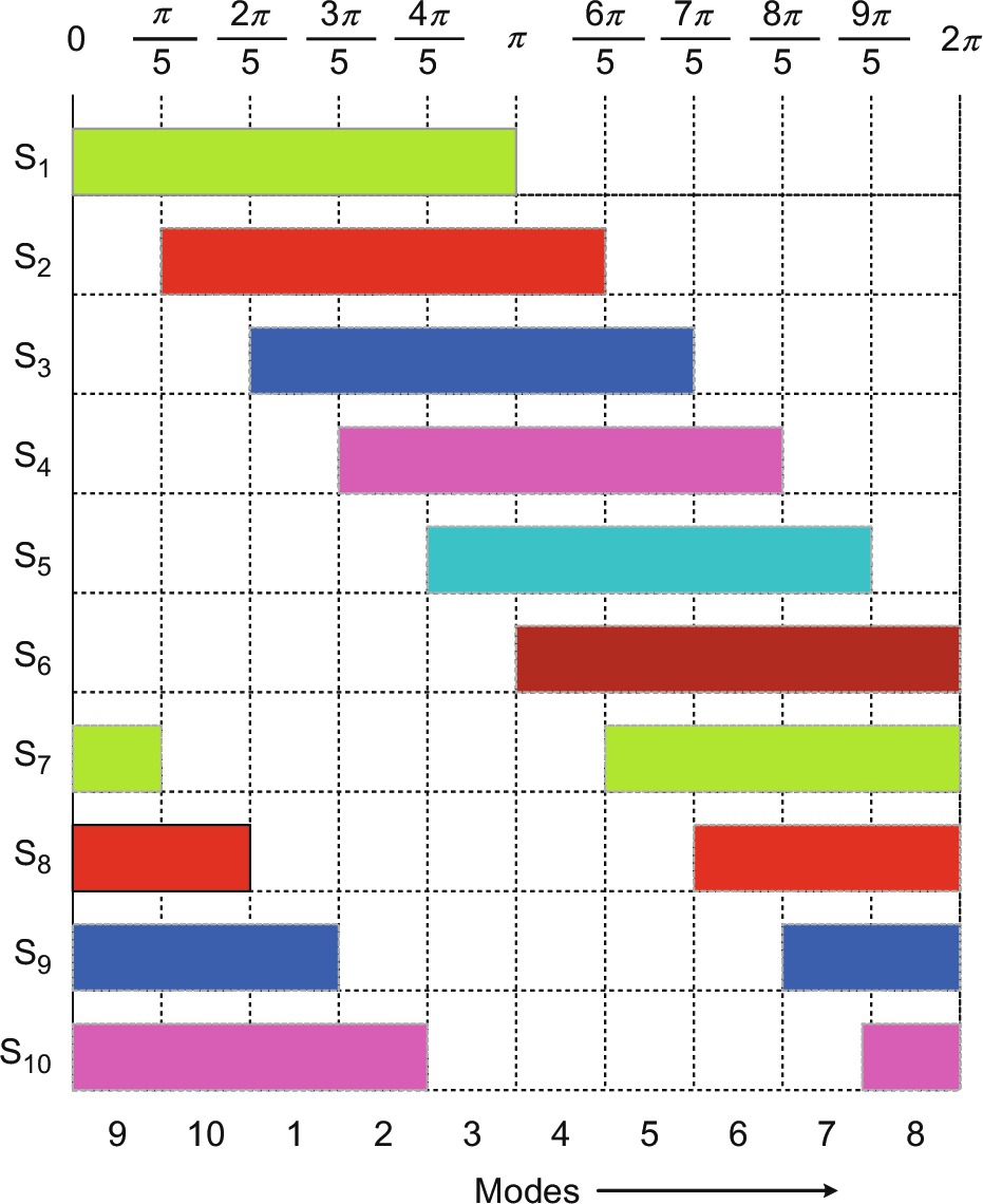
Table 15.2
Modes of operation of the five-phase voltage-source inverter (10-step operation)
| Mode | Switches ON | Terminal polarity |
| 1 | 9,10,1,2,3 | A+B+C-D-E+ |
| 2 | 10,1,2,3,4 | A+B+C-D-E- |
| 3 | 1,2,3,4,5 | A+B+C+D-E- |
| 4 | 2,3,4,5,6 | A-B+C+D-E- |
| 5 | 3,4,5,6,7 | A-B+C+D+E- |
| 6 | 4,5,6,7,8 | A-B-C+D+E- |
| 7 | 5,6,7,8,9 | A-B-C+D+E+ |
| 8 | 6,7,8,9,10 | A-B-C-D+E+ |
| 9 | 1,7,8,9,10 | A+B-C-D+E+ |
| 10 | 8,9,10,1,2 | A+B-C-D-E+ |
Space vector of phase voltages in stationary reference frame is defined, using power variant transformation [33]:
v¯=25(va+a¯vb+a¯2vc+a¯*2vd+a¯*ve)
where a=exp(j2π/5), a2=exp(j4π/5), a⁎=exp(−j2π/5), a⁎2=exp(−j4π/5), and ⁎ stands for a complex conjugate.
Leg voltages (i.e., voltages between points A,B,C,D, and E and the negative rail of the DC bus N in Fig. 15.26) are considered first. The leg voltages from Fig. 15.27 are substituted in expression (15.68) to obtain their corresponding space vectors given as in Eq. (15.69):
[→v1leg→v2leg→v3leg→v4leg→v5leg→v6leg→v7leg→v8leg→v9leg→v10leg]=25VDC(2cosπ5)[ej0ejπ/5ej2π/5ej3π/5ej4π/5ejπej6π/5ej7π/5ej8π/5ej9π/5]

It is seen that the leg voltages have magnitude of 25VDC2cos(π/5)![]() and are 36 degrees apart forming a decagon. There are in total 25=32 switching states (base is taken as 2 because the switching states can only assume two values either 0 (indicate off state) or 1 (indicate on state)). The first 10 states are described above, and the remaining 22 switching states are discussed in the next section.
and are 36 degrees apart forming a decagon. There are in total 25=32 switching states (base is taken as 2 because the switching states can only assume two values either 0 (indicate off state) or 1 (indicate on state)). The first 10 states are described above, and the remaining 22 switching states are discussed in the next section.
Phase-to-neutral voltages are discussed next. Phase-to-neutral voltages of the star-connected load are most easily found by defining a voltage difference between the star point n of the load and the negative rail of the DC bus N. The following correlation then holds true:
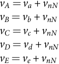
vA=va+vnNvB=vb+vnNvC=vc+vnNvD=vd+vnNvE=ve+vnN
Since the phase voltages in a star-connected load sum to zero (sum of five-phase sine wave at one instant of time is zero), the summation of Eq. (15.70) produces
vnN=(1/5)(vA+vB+vC+vD+vE)
Substitution of (15.71) into (15.70) produces phase-to-neutral voltages of the load in the following form:
va=(4/5)vA−(1/5)(vB+vC+vD+vE)vb=(4/5)vB−(1/5)(vA+vC+vD+vE)vc=(4/5)vC−(1/5)(vA+vB+vD+vE)vd=(4/5)vD−(1/5)(vA+vB+vC+vE)ve=(4/5)vE−(1/5)(vA+vB+vC+vD)

The phase voltages in different modes are obtained by substituting leg voltages into Eq. (15.72), and their space vectors are determined using Eq. (15.68). The space vectors of phase-to-neutral voltage are identical to the leg voltage space vectors. The phase-to-neutral voltages for various modes are given in Fig. 15.28.

Fourier analysis of the voltage waveforms, which relates DC link voltage of the inverter with the output, is elaborated.
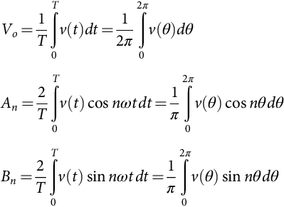
Using the definition of the Fourier series for a periodic waveform,
v(t)=Vo+∞∑n=1(Ancosnωt+Bnsinnωt)

where the coefficients of the Fourier series are given with
Vo=1TT∫0v(t)dt=12π2π∫0v(θ)dθAn=2TT∫0v(t)cosnωtdt=1π2π∫0v(θ)cosnθdθBn=2TT∫0v(t)sinnωtdt=1π2π∫0v(θ)sinnθdθ
Observing that the waveforms possess quarter-wave symmetry and can be conveniently taken as odd functions, one can represent phase-to-neutral voltages with the following expressions:
v(t)=∞∑n=1B2n−1sin(2n−1)ωtwhereB2n−1=4ππ2∫0v(θ)sin(2n−1)θdθandn=1,2,3,…

In the case of the phase-to-neutral voltage vb, shown in Fig. 15.28, one further has for the coefficients of the Fourier series:
B2n−1=8VDC5π(2n−1)[1+cos(2n−1)3π5cos(2n−1)4π5]wherek=1,2,3,…

The expression in brackets of Eq. (15.76) equals zero for all the harmonics whose order is divisible by five. For all the other harmonics, it equals 2.5. Hence, one can write the Fourier series of the phase-to-neutral voltage as
v(t)=2πVDC[sinωt+13sin3ωt+17sin7ωt+19sin9ωt+111sin11ωt+113sin13ωt+…]

From (15.77), it follows that the fundamental component of the output phase-to-neutral voltage has an rms value equal to
V1=√2πVDC=0.45VDC

From Fig. 15.28, mean square value is determined as
Meansquarevalue=1π[(25VDC)2×3π5+(35VDC)2×2π5]=625V2DC
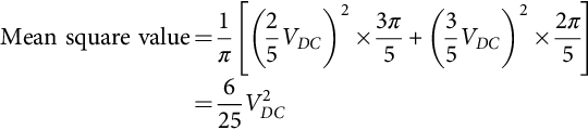
Vrms=√65VDC

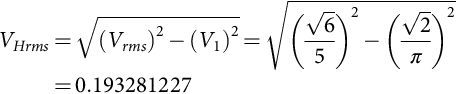
Total harmonic rms voltage (per unit) is given by
VHrms=√(Vrms)2−(V1)2=√(√65)2−(√2π)2=0.193281227
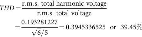
Hence, total harmonic distortion is
THD=r.m.s.totalharmonicvoltager.m.s.totalvoltage=0.193281227√6/5=0.3945336525or39.45%
This is the same voltage as obtainable with a three-phase VSI operating in six-step mode. It is important to note at this stage that the space vectors described by (15.68) provides mapping of inverter voltages into a two-dimensional space. However, since five-phase inverter essentially requires description in a five-dimensional space, not all the harmonics contained in (15.77) will be encompassed by the space vector of (15.68). In particular, space vectors calculated using (15.68) will only represent harmonics of the order 10k±1,k=0,1,2,3…![]() , that is, the first, the ninth, the eleventh, and so on. Harmonics of the order 5k,k=1,2,3…
, that is, the first, the ninth, the eleventh, and so on. Harmonics of the order 5k,k=1,2,3…![]() cannot appear due to the isolated neutral point. However, harmonics of the order 5k±2,k=1,3,5…
cannot appear due to the isolated neutral point. However, harmonics of the order 5k±2,k=1,3,5…![]() are present in (15.77) but are not encompassed by the space-vector definition of (15.68). These harmonics in essence appear in the second two-dimensional space, which requires introduction of the second space vector for the five-phase system.
are present in (15.77) but are not encompassed by the space-vector definition of (15.68). These harmonics in essence appear in the second two-dimensional space, which requires introduction of the second space vector for the five-phase system.
Simulation is performed to obtain the harmonic spectrum of inverter phase voltage in 10-step mode of operation, shown in Fig. 15.29. The DC voltage is kept at 1 p.u. The harmonic spectrum is in compliance with the expression (15.77) and (15.78).

The fundamental component is equal to 0.4504 pu, which is the same as what is obtainable with a three-phase VSI. The subharmonic components are third and seventh in Fig. 15.29, and their magnitudes are 33.33% and 14.3%, respectively. These subharmonics will appear in the x-y plane and will cause distortion in the stator currents and consequently increase the losses in the machine. The lowest harmonic appearing on d-q plane are 9th and 11th with their magnitude as 11.1% and 9.1%, respectively. These harmonic will further add to the losses in addition to 10th-harmonic pulsating torque under steady-state conditions.
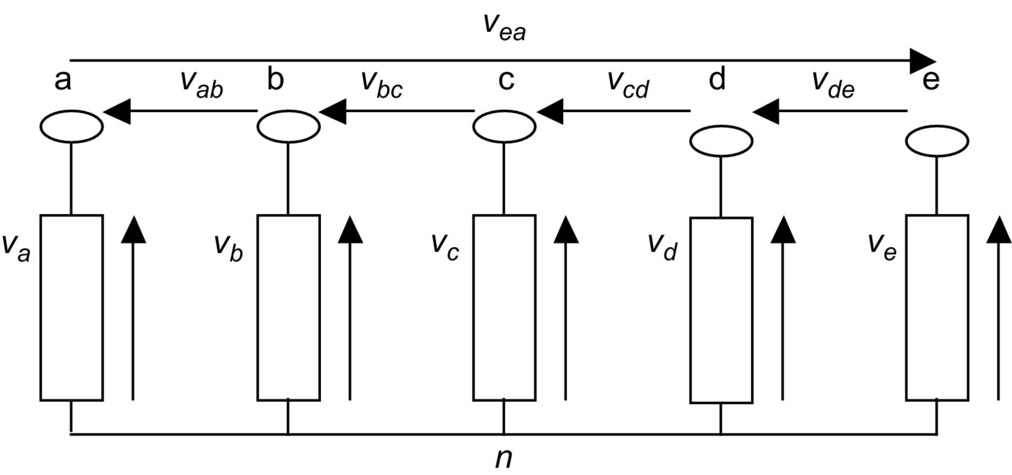
The line-to-line voltages are expanded next. There are two systems of line-to-line voltage, adjacent and nonadjacent, in contrast to a three-phase system where only one line-to-line voltage is defined. The adjacent line-to-line voltages at the output of the five-phase inverter are defined in Fig. 15.30, for a fictitious load. Since each line-to-line voltage is a difference of corresponding two leg voltages, the values of nonadjacent line-to-line voltages will produce higher magnitude compared with the adjacent line voltages; hence, only former case is taken up in the thesis and later is omitted from further consideration.
There are two sets of nonadjacent line-to-line voltages. Due to symmetry, these two sets lead to the same values of the line-to-line voltage space vectors, with a different phase order. Only the set vac,vbd,vce,vda,veb is analyzed for this reason. Table 15.3 lists the states and the values for these line-to-line voltages.
Table 15.3
Nonadjacent line-to-line voltages for 180 degrees conduction mode
| Switching state | Switches ON | Space vector | vac | vbd | vce | vda | veb |
| 1 | 9,10,1,2,3 | v1ll | VDC | VDC | −VDC | −VDC | 0 |
| 2 | 10,1,2,3,4 | v2ll | VDC | VDC | 0 | −VDC | −VDC |
| 3 | 1,2,3,4,5 | v3ll | 0 | VDC | VDC | −VDC | −VDC |
| 4 | 2,3,4,5,6 | v4ll | −VDC | VDC | VDC | 0 | −VDC |
| 5 | 3,4,5,6,7 | v5ll | −VDC | 0 | VDC | VDC | −VDC |
| 6 | 4,5,6,7,8 | v6ll | −VDC | −VDC | VDC | VDC | 0 |
| 7 | 5,6,7,8,9 | v7ll | −VDC | −VDC | 0 | VDC | VDC |
| 8 | 6,7,8,9,10 | v8ll | 0 | −VDC | −VDC | VDC | VDC |
| 9 | 7,8,9,10,1 | v9ll | VDC | −VDC | −VDC | 0 | VDC |
| 10 | 8,9,10,1,2 | v10ll | VDC | 0 | −VDC | −VDC | VDC |

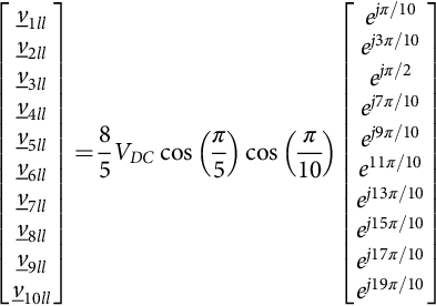
Space vectors of nonadjacent line-to-line voltages are determined once more using the defining expression (15.68) and are summarized as
[v¯1llv¯2llv¯3llv¯4llv¯5llv¯6llv¯7llv¯8llv¯9llv¯10ll]=85VDCcos(π5)cos(π10)[ejπ/10ej3π/10ejπ/2ej7π/10ej9π/10e11π/10ej13π/10ej15π/10ej17π/10ej19π/10]
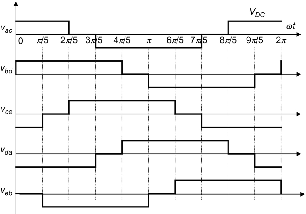
Time-domain waveforms of nonadjacent line-to-line voltages are illustrated in Fig. 15.31.
The Fourier analysis is further carried out for nonadjacent line-to-line voltage following the same procedure outlined in conjunction with Fourier analysis of phase voltages. The nonadjacent line voltages waveform possess quarter-wave odd symmetry; hence, the Fourier coefficient can be evaluated as
B2n−1=4VDC(2n−1)π(cos(2n−1)π10)wheren=1,2,3,…

And the Fourier series of nonadjacent line-to-line voltage can be written as
vll(t)=4πVDC[cos(π10)sin(ωt)+13cos(3π10)sin(3ωt)+17cos(7π10)sin(7ωt)+…]
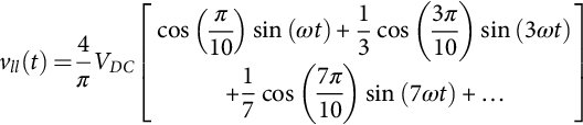
Thus, the peak of the fundamental is
Vll=4πVDCcos(π10)=1.211VDC
From Fig. 15.31, mean square value is determined as
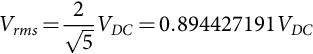
Meansquarevalue=1π[(VDC)2×4π5]=45V2DC
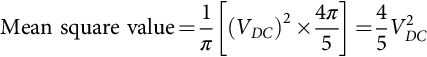
Vrms=2√5VDC=0.894427191VDC
Total harmonic rms voltage (pu) is given by