
Thermal Modeling and Analysis of Power Electronic Components and Systems
Peter R. Wilson University of Bath, Bath, United Kingdom
Abstract
This chapter will introduce some basic techniques for modeling thermal circuits using lumped equivalent circuits that can be used in power electronic circuits. The fundamental thermal circuit concepts are introduced, and the methods by which these can be used in a practical manner by the power electronics designer are discussed.
Keywords
Device modeling; Magnetic components; Thermal conduction; Convection; Radiation; Thermal modeling; Transient thermal impedance; Numerical methods
46.1 Introduction
In the field of power electronics, most of the challenges arise from the thermal management and our ability to predict the behavior of circuits under varied and extreme temperature conditions. It is particularly important in power electronics to understand the effects of temperature as this fundamentally affects so many aspects of the design from component values to tolerances, reliability, performance, and robustness. This chapter will therefore focus on understanding how to model and analyze thermal models relating to power electronic components and systems.
Heat is transported by three main mechanisms, conduction, convection, and radiation [1], and all three mechanisms can be important in power electronics, although the first two are generally the most significant. Heat transport occurs in three dimensions, which can make detailed analysis difficult; therefore one objective in modeling thermal behavior in power electronic systems is to reduce the problem to a simpler level and make it easier for the designer to get approximate but sufficiently accurate answers to design questions. A particular issue for the power electronics designer is that not only is the thermal behavior a requirement to accurately model the system but also is the interdependence with the device behavior. Power devices contribute heat due to losses and switching behavior, and this also contributes to self-heating effects that fundamentally affect their behavior. In some devices, this can become a serious problem. In power electronic circuits, there are also significant effects due to the variability of passive components such as resistance, capacitance, and magnetic components due to temperature, and these must all be taken into account when understanding the overall circuit behavior in this context. Finally, the environment temperature will also have a major impact on the performance of the power electronic circuit, and an effective and efficient approach is required to modeling such thermal effects.
46.2 Background
Modeling and simulation of thermal effects has been at the heart of power electronics for many years, with engineers attempting to understand fundamental device behavior needing to understand specific thermal behavior to provide model parameters that would accurately reflect the true model behavior [2,3]. Using simple thermal resistance and capacitance models (discussed in more detail later in this chapter) either integrated in the device models [4] or extending the SPICE simulator to include thermal effects directly in the models [5], the use of equivalent “lumped element” models has been used for more than 25 years to improve our understanding of temperature and its effect on semiconductor device operation. This has been a particular issue for the bipolar device community due to the “thermal runaway” characteristics of these devices; however, the use of similar techniques by the power electronics community has become common [6]. This is still an ongoing research issue primarily due to the difficulty of accurately obtaining thermally dependent parameters for the device and package thermal circuit and also making empirical measurements that can confirm the validity of the approach. In this chapter, we will look at some techniques that can be applied to modeling thermal behavior and some approaches to implement some form of modeling to understand at least the basic thermal behavior of power electronic devices and systems.
46.3 Semiconductor Device Modelling
Simulation Program with Integrated Circuit Emphasis (SPICE) building block models exist for diodes and MOSFETs in most circuit simulators already, but they were generally designed for low-voltage and small current integrated circuit applications as the name of the program suggests. They do not (usually) have bulk effects or dynamic thermal behavior, which is essential for power electronics. Like any semiconductor device power diode, MOSFETS and IGBTs are highly nonlinear and depend fundamentally on temperature. If we consider the humble diode equation (46.1),
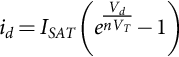
Eq. (46.1) relates the diode current in a nonlinear fashion to the diode voltage where ISAT is the saturation current, Vd is the junction voltage, VT=kT/q is the thermal voltage, and n is the emission coefficient. It is obvious that the thermal voltage depends directly on the temperature. This type of approach has been used in SPICE (and other circuit simulators for many years), where the simulator temperature is defined as a global variable and used in semiconductor device models, with the assumption being that the circuit will be in a thermal steady state and this can be defined precisely by the designer. In some simulators, such as SABER, the temperature can be defined hierarchically so that a circuit or even device can have a unique temperature, but this is still effectively static. A breakthrough was to make the temperature of the device a dynamic variable that could be modeled using a thermal circuit at the same time as the electric circuit, and by using electric analogies, the integrated device behavior could be made more accurate.
Another key issue with the modeling power devices was to take a different approach to that of the low-power IC designers and to create models of power devices such as diodes, MOSFETs, and IGBTs that were more appropriate to this context. This was the “lumped-charge” approach [7], and this model handles the forward and reverse recovery characteristics much better than the basic low-voltage model. It has been implemented in Saber for more than 20 years, and the general approach has been extended to a wide variety of power semiconductor models [8] and to other simulators such as Modelica [9].
Often, power electronics designers do not understand the detail of model that is required to solve their design problem, and this relates directly to the implementation of a thermal model too. This can be encapsulated in a series of questions such as the following:
• Do you need a detailed physics model?
• Do you need cycle by cycle accuracy?
• Can you characterize the data well enough to achieve the accuracy?
These questions (and the answers to them) will often dictate the type of model to be used and the resulting complexity of system to analyze.
46.4 Magnetic Components
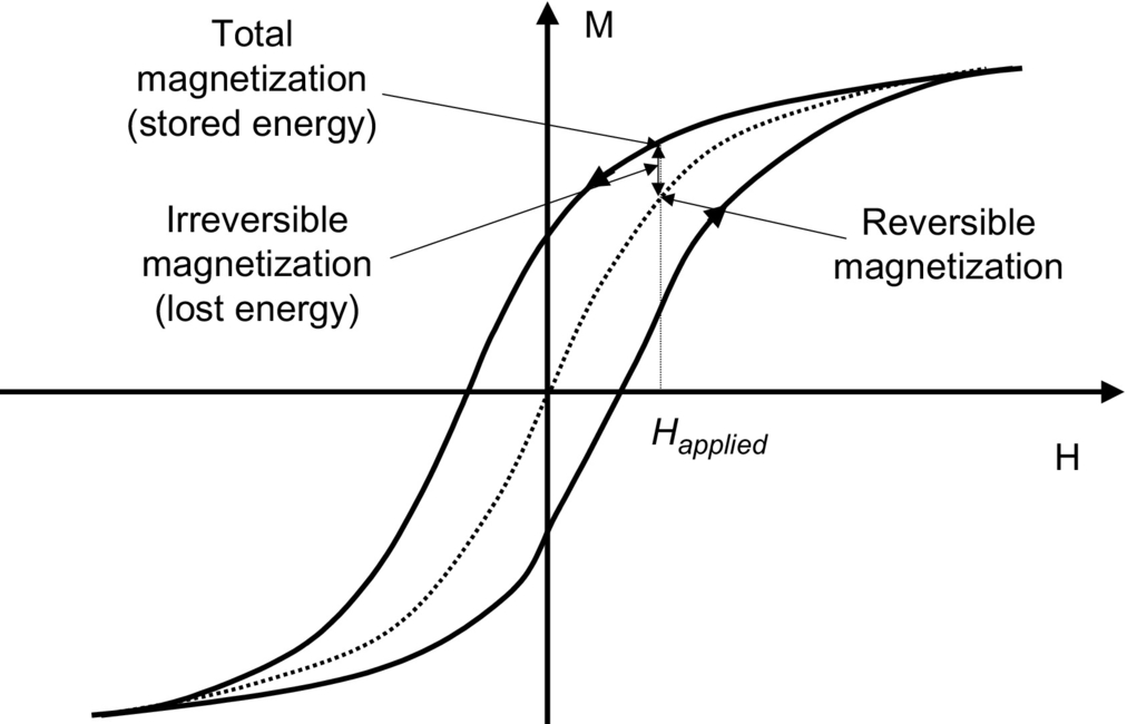
Magnetic components that include a nonlinear ferrite core are some of the most difficult to model in a power electronic system. The nonlinear BH curve that defines the magnetic behavior of the inductors and transformers in a power electronic system has a profound effect on the behavior of the system as a whole. It is also highly thermally dependent, and therefore, it is useful to be able to model this.
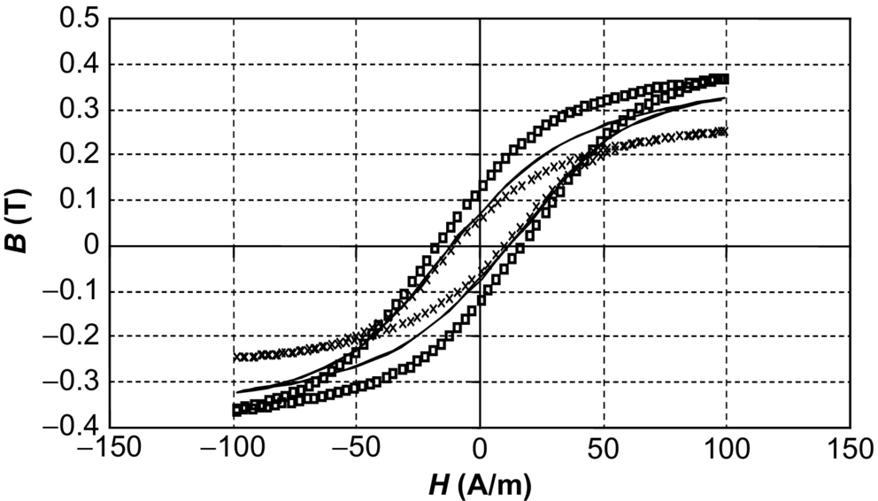
A basic BH curve is shown in Fig. 46.1, and this illustrates the effect of high magnetic field strength (causing saturation) and the remanence effect that leads to hysteresis. This is difficult enough to model without thermal effects (e.g., see the Jiles-Atherton approach [10–12]), and this has been implemented in most circuit simulators; however, the problem for power electronic circuit designers is that the BH curve can vary with temperature as shown in Fig. 46.2.
This can be managed in a simulation model by not only including a thermal pin, in a similar manner to the power semiconductor devices, but also making it self-heating to take into account eddy currents or losses that contribute to the overall thermal behavior [13].
In order to understand the methods of integrating thermal behavior into power electronic circuits, it is useful to first review the principles in thermal modeling.
46.5 Thermal Conduction
The conduction of heat through materials is by far the simplest transport mechanism to analyze. The transport of heat with conduction is described by the Fourier heat equation given in Eq. (46.1):
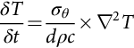
where ρ is the density and c is the specific heat. The heat flux (power flow per unit area) can be found at any point using Eq. (46.3):
As with all partial differential equations, the solution of the Fourier equation can only be performed exactly for a few simple sets of boundary and initial conditions. Solutions can be found numerically or using approximate methods if we consider the conduction of heat through a square plate of area A and thickness d as shown in Fig. 46.3.

The two surfaces are at uniform temperatures T1 and T2. If it is the case that d≪A, then we can make the assumption that the heat loss from the edges may be neglected and the resulting heat flow is in one dimension. The heat flow through the plate can therefore be calculated using Eq. (46.4):
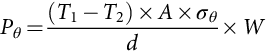
where σθ is the thermal conductivity. Notice the use of the subscript θ to emphasize that both the power and conductivity are thermal. Eq. (46.4) is often written in the form shown in Eq. (46.5):
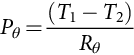
where Rθ is the thermal resistance of the plate, given by Eq. (46.6):
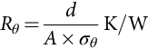
It is useful to see that the magnitude of thermal resistances for commonly used materials (in this case assuming a plate of area 10−4 m2 (1 cm×1 cm) and thickness 1 mm) is shown in Table 46.1.
Table 46.1
Thermal conductivity and resistance of a range of materials
| Material | Thermal conductivity (W/K/m) | Thermal resistance (K/W) |
| Aluminum | 217 | 0.046 |
| Copper | 394 | 0.025 |
| Gold | 291 | 0.034 |
| Lead | 34.3 | 0.29 |
| Tin | 63 | 0.16 |
| PCB (FR4) | 0.3 | 33 |
| Alumina | 27.6 | 0.36 |
| Diamond | 630 | 0.016 |
| Silicon | 150 | 0.067 |
| GaN | 130 | 0.077 |
| Silicon carbide | 500 | 0.02 |
Table 46.1 is interesting in that as we might expect, copper is an extremely good conductor; however, it is particularly interesting to look at three common materials for power electronic devices, silicon, gallium nitride, and silicon carbide. They all have excellent thermal properties; however, silicon carbide is particularly good making it advantageous for power electronic applications where thermal management is crucial.
The equation for conduction of heat has the same form as Ohm's law, making it easy to draw a direct analogy between the thermal and electric resistance equations:

The analogy is drawn that P is equivalent to I, T is equivalent to V, and Rθ is equivalent to R. T in the thermal model is defined as an across variable, that is, only differences between points are specified. This means that as for voltage, there must be a reference node. This is usually the ambient temperature, Ta. P is a through variable in the same that in an electric circuit, current must flow around a closed loop.
46.6 Convection
Convection is the process by which heat is transferred from a solid surface to a nonsolid, such as air or water. The convection process involves the motion of the fluid relative to the solid surface and the processes by which heat is transferred across the interface.
There are two main forms of convection, natural or free convection, where the motion of the fluid is produced by the change in density with temperature, and forced convection, where the motion is generated by an external mechanism, a fan or a pump.
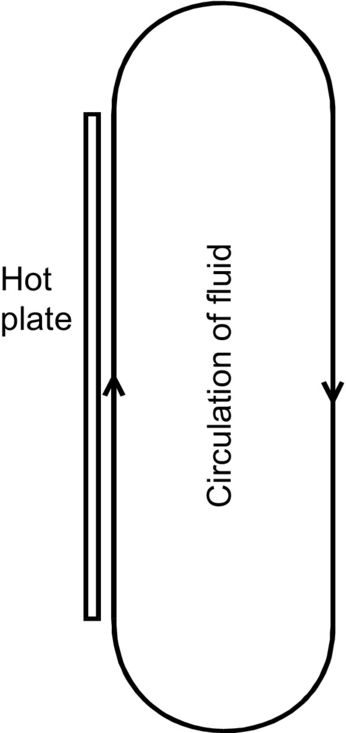
Convection is most effective where the hot surface is vertical. The air is heated by the plate and rises by the “chimney effect.” Forced airflow parallel to the plate will increase heat transfer. Heat transfer will depend on surface area, height, and temperature difference (Fig. 46.4). The process of convection is complex and not readily amenable to analysis; therefore, empirical methods have been developed, allowing models to be created based on these measurements.
46.7 Radiation
The final concept of heat transfer is radiation. In this context, radiation refers to the transfer of heat by electromagnetic radiation. The basic equation for heat transfer by radiation is the Stefan-Boltzmann law that is given in Eq. (46.8):
where T is the absolute temperature of the radiating surface (K), Ta is the ambient temperature of the surrounding objects (K), A is the area (m2), and E is a constant known as the emissivity. The emissivity may vary from as low as 0.05 for polished aluminum to 0.9 for black oxidized aluminum.
In order to put the power loss by radiation into context, consider a 1 cm2 black anodized aluminum plate. The plate is at a temperature of 373 K, and the ambient temperature is at 323 K.
Taking into account the heat loss from both sides of the plate, the power loss is given by Eq. (46.9):
With a heat sink using natural convection, radiation will play a role in removing heat. The difference between a shiny aluminum heat sink and the same sink anodized black is of order 5%–25%, and the advantage rises with temperature.
Now, we have covered the basics of thermal behavior; we can investigate how to implement useful models for inclusion in power electronic circuits.
46.8 Steady State Thermal Circuit Modeling
For the thermal circuit model to be of use, it must be possible to define the temperature at well-defined points that are defined as the nodes of the thermal circuit. It must also be possible to define the heat flux and thermal resistance between these points, which implies that we therefore have a lumped model. At this stage, we are considering the steady state only, where the temperatures have stabilized into an equilibrium condition.
It is essentially the same as describing an electric circuit in terms of nodes connected by electric components, which is valid as long as it is not necessary to consider distributed effects (such as a transmission line). The lumped components in the thermal circuit are generally less well defined than their electric counterparts, due to the uncertainty in characterization of the thermal parameters and approximations made to obtain the parameters.
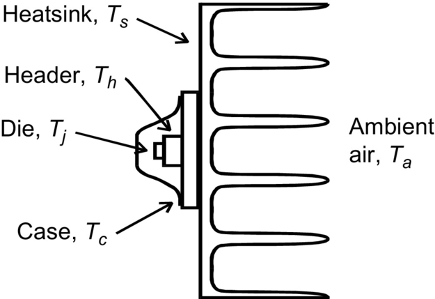
If we consider the example of a transistor that is bolted to a heat sink, as shown in Fig. 46.5, we can see that there are five temperatures to consider in this model, starting from the junction temperature of the device (Tj), the header temperature (Th), the case temperature (Tc), the heat sink (Ts), and finally the ambient temperature (Ta).
The heat flow into the thermal circuit from the device is the power dissipation (in watts) from the power device, which is analogous to current in the electric domain. At this point, the obvious question is how do we model this thermal circuit in such a way that we can calculate all the intermediate temperatures based on a power dissipation value from the power transistor? We can represent each of the individual thermal elements as a thermal resistance connected in series with a thermal heat source as shown in Fig. 46.6.
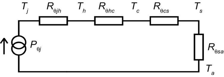
In this example, the thermal circuit has been represented by four resistors with five nodes. In practice, Rqjh and Rqhc would not readily be measured separately and so would be grouped together as Rqjc, a parameter measured by the manufacturer. The heat-sink supplier would specify Rqsa, and the contact resistance between case and heat sink would depend on mounting method surface conditions. The junction temperature can be estimated using Eq. (46.10):
and the heat-sink temperature can also be estimated from Equation (46.11):
This lumped approach starts to become very effective when the situation becomes more complex as it can be easily modeled using SPICE or other circuit simulators, such as the case when there are several devices mounted on the same heat sink as shown in Fig. 46.7.
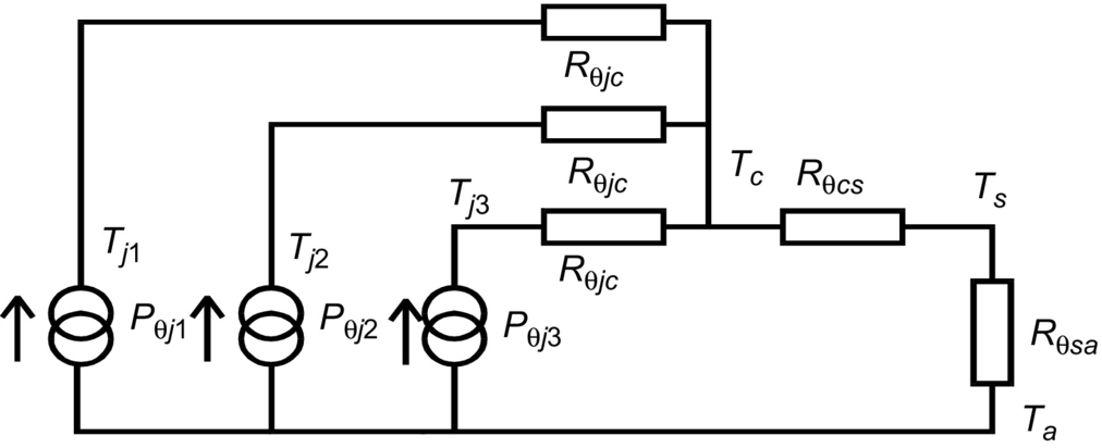
This circuit can quickly be solved and the resulting heatsink temperature estimated.
46.9 Dynamic Thermal Circuit Modeling
So far, only steady-state thermal circuits have been considered. There are however many situations where it is required to model the transient behavior, such as when the dynamic electric behavior changes (say under peak inrush current conditions or a failure current). When heat is applied to an object, the temperature will increase at a rate determined by the heat input and the thermal capacity of the object. Although the scenario has moved from steady state to dynamic, the assumption is still being made that a single temperature may be assigned to the object, that is, a lumped model rather than a distributed one. This will not necessarily be the case, but it is a necessary assumption for the lumped component model. Generally, some kind of average temperature will be used. The thermal capacity of a lumped component of the thermal circuit is given by Eq. (46.12):
where m is the mass of the component and cs the specific heat of the material. In terms of the circuit model, the thermal capacity is analogous to an electric capacitor. A transistor on a heat sink may therefore be represented by Fig. 46.8.

This model is useful, but there are still issues to resolve. If we consider the heat sink, a thermal capacity Rθs has been ascribed to it, and this is relatively well defined. In the model, the temperature drop across the heat sink itself has been neglected. The thermal resistances either side of the capacitor are interface resistances, with no significant thermal capacity. Similarly, the case presents a relatively large thermal capacity but little thermal resistance. The header and the die however are different. Here, they have both been considered as two lumped components. This is not a very good assumption as in reality the thermal resistance and thermal capacity in both header and die are distributed.
46.10 Approximating Distributed Thermal Behaviour Using Ladder Networks
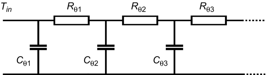
One solution to the problem of approximating a distributed thermal network is to use a thermal ladder network. The thermal resistance is divided into n sections of Rθ/n and the capacitance into n capacitances of value Cθ/n. This is exactly the same problem that arises in distributed electric networks (such as transmission lines), and the same approach may be taken as shown in Fig. 46.9. However, it should be noted that there is no obvious equivalent to an inductance in the thermal domain.
46.11 Transient Thermal Impedance
The ladder network approach is useful but is a hard work to analyze. A simpler approach is needed and that approach is the transient thermal impedance. When considering active devices mounted on a heat sink, the external part can be adequately described by the simple thermal resistance—thermal capacity concept. The problem area is the internal behavior of the device. The central idea is to replace the internal thermal resistance by a thermal impedance that depends on the temporal variation of the power dissipated. The objective is to accurately estimate the maximum junction temperature.
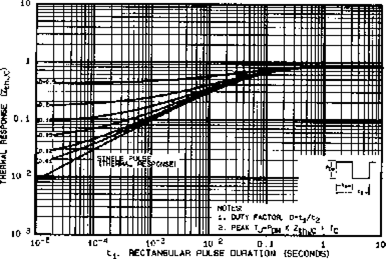
A typical data sheet graph (for the International Rectifier IRF 450 n-type power MOSFET in a modified TO-3 package, a 500 V 12 A device) of thermal impedance is shown in Fig. 46.10, with the thermal impedance plotted against the pulse duration on the x-axis and the family of curves showing how the duty ratio affects the effective thermal impedance, normalized to the thermal resistance. For this device, the thermal resistance is found on the data sheet as the parameter RthJC and is 0.83°C/W, and the junction to ambient thermal resistance is 30°C/W. (For comparison, a TO-240 package—device is denoted by IRFM450—has a junction to ambient thermal resistance of 48°C/W.)
The starting point is the response of the junction temperature to a unit step of input power, when the case temperature is constant. The temperature after a time t is the equivalent of the maximum temperature reached by the junction for a single pulse of duration t. The steady-state response is a rise of temperature equal to the thermal resistance Rqjc.
The dynamic response of the junction temperature can be seen in Fig. 46.11, where the temperature will rise smoothly to the steady-state value.

The rise of junction temperature above the case temperature for a pulse of length t is defined as the thermal impedance for a pulse of length t. This is for a pulse of unit height. If the pulse has an amplitude Pm and duration t, the maximum junction temperature is given by Eq. (46.13):
If the pulses are repetitive with a duration t and duty ratio D (Period t/D), the maximum temperature will rise above the value for a single pulse of duration t as shown in Fig. 46.12.
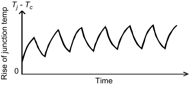
With multiple pulses, the temperature oscillates, the magnitude of the oscillation decreasing with increasing frequency. In the limit, the ripple will approach zero, with a temperature rise corresponding to the mean power (Pm×D) multiplied by the thermal resistance. Measured values for thermal impedance can be seen on manufacturer's data sheets. The graphs show the thermal impedance normalized to the thermal resistance, as a function of pulse width and duty ratio.
46.12 Procedure to Calculate the Transient Thermal Impedance
The procedure to use thermal impedance to calculate the temperature difference between junction and case starts by calculating the approximate power pulse by an equivalent square pulse of equal area and same height based on the actual pulse as shown in Fig. 46.13. From this figure, it is possible to deduce equivalent pulse width, teq. The way to do this is to estimate the area under the actual curve (using a trapezoidal approach) and from the maximum value calculate the equivalent pulse width based on the rectangular area required. The duty ratio can then be calculated based on the ratio of the equivalent pulse width and the switching period.
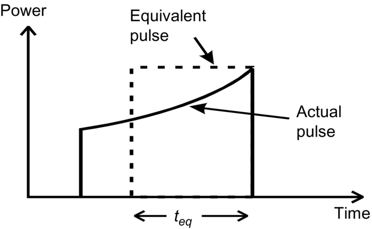
With the equivalent pulse width and the derived duty ratio, the graph of thermal impedance can be used to look up the appropriate value.
The maximum difference (effectively the steady state) can then be calculated by multiplying the peak pulse power by the value of thermal impedance obtained from the data sheet. In practice, the pulsing thermal behavior we see in Fig. 46.12 will be filtered out by the time the case is taken into account, and the calculation of case temperature may be made using the average power and the external thermal resistances.
46.13 Finite Element Numerical Methods
The solution of the Fourier heat equation in anything but the simplest cases requires the use of numerical methods such as the finite element method. For the steady state, the Fourier equation reduces to the Laplace equation in Eq. (46.14):
and the heat flux (power per unit area) at any point is given by Eq. (46.15):
The Laplace equation occurs in many physical systems, and the solution of it is a standard problem; however, due to the complexity of most real-world systems, finite element techniques are the preferred technique to obtain a numerical solution. Solutions for the temperature distribution in physical geometries can be obtained using commercial software packages designed to implement the finite element method. In most cases, this will give the equilibrium or steady-state solution rather than the transient behavior. In order to calculate, the transient thermal distribution requires the use of repeated finite element simulations for different initial conditions and applied heat flow values (as in the pulsed example shown in Fig. 46.13). This can take a high level of computation to complete and for complex geometries can take a long time to complete.
46.14 Dynamic Thermal Equivalent Circuit Models
When the calculations get more complex than a simple junction to case and junction to ambient calculation, then the choice for the power electronics design engineer is to either create a complex geometric model for the device, case, heat sink, and environment and then conduct extensive, repeated finite element analyses or more commonly use equivalent circuit models instead.
One obvious circuit that is often used to provide an increased level of detail, which effectively approximates the finite element model in one dimension, is the ladder circuit. For example, if we take the IRF450 device we have looked at previously, we can see that the junction to case thermal resistance RthJC is 0.83°C/W; therefore, if we create a 10-section RC ladder network, then each individual thermal resistance will be 0.083 C/W (one-tenth of the overall thermal resistance). In the steady state, this will be identical to the lumped model we looked at previously in this chapter (Fig. 46.14). It is possible to calculate an appropriate value for the ladder capacitances; however, in most cases, it is just as quick (and certainly easier) to use a simulation to experiment with the capacitance values to obtain the best matching of time dependence with the data for the device.
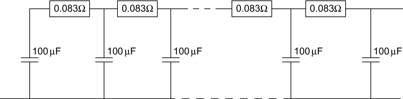
If a heat flow (current in an electric analogous circuit) is applied, then the voltage will represent the thermal impedance over time, and this can be matched to the data sheet transient thermal impedance. For example, using the Saber simulator, we can define a thermal circuit using dedicated thermal resistance and capacitance models (although we could equally well use SPICE models for electric analogues), as shown in Fig. 46.15.
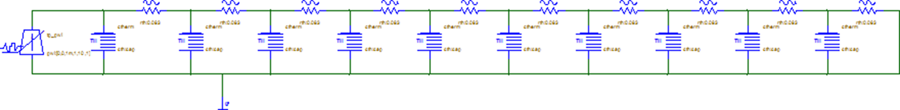
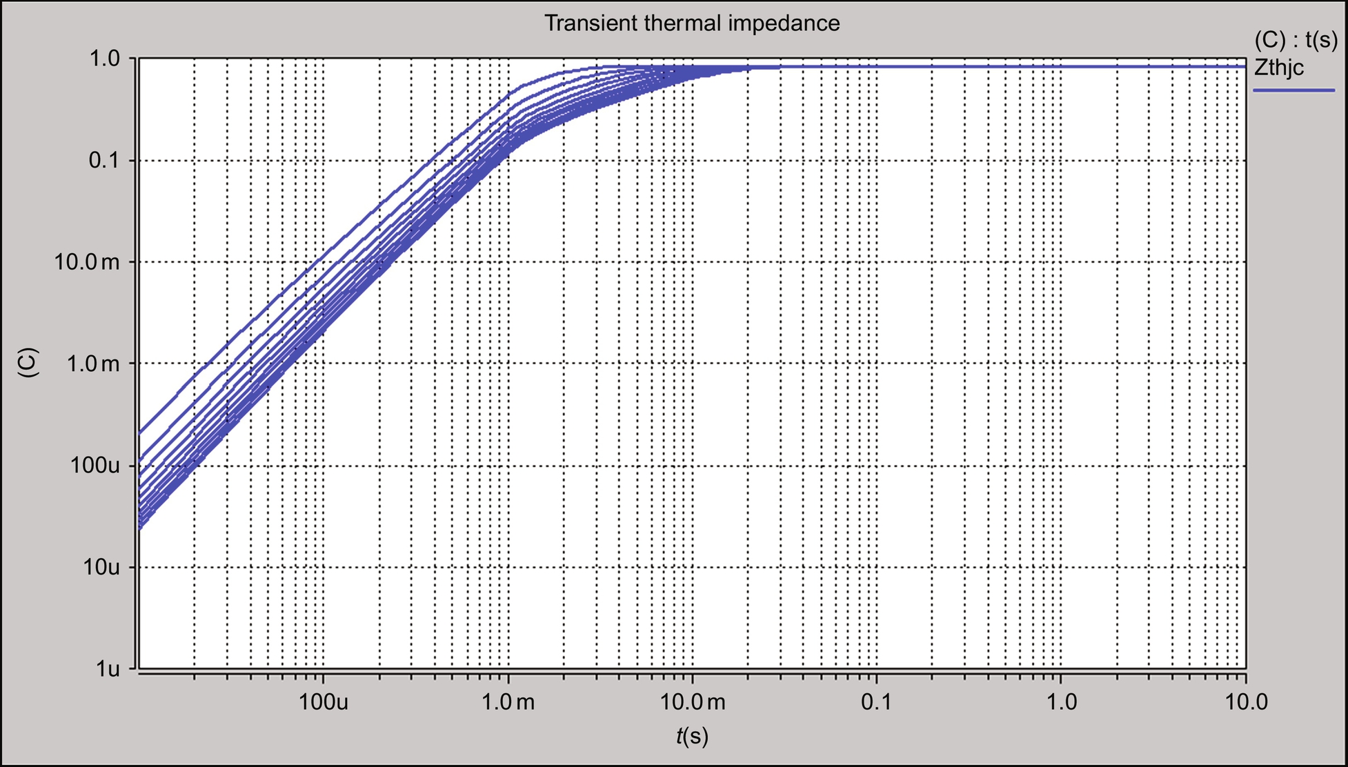
Varying the capacitance value allows the response of the transient thermal impedance to be obtained from the temperature across the whole ladder network. In this case, we can vary the capacitance on each leg from 200 to 2000 μF, with the resulting responses as shown in Fig. 46.16.
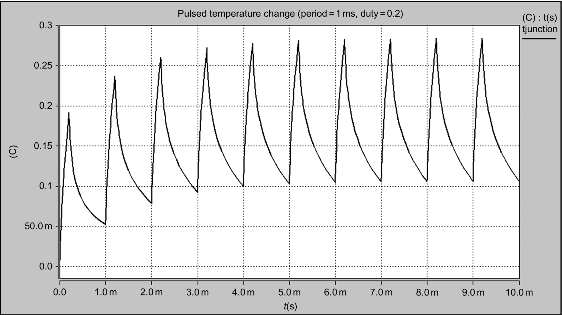
The same circuit can be used to test the behavior of the thermal circuit to a pulsed heat source, much as would be the case when a power device is switched on and off, and we can simulate this using the same test circuit, but with a pulse heat source (Fig. 46.17). Using a period of 1 ms and a duty ratio of 0.2, we can see the temperature response as follows (when the capacitance is defined as 400 μF).
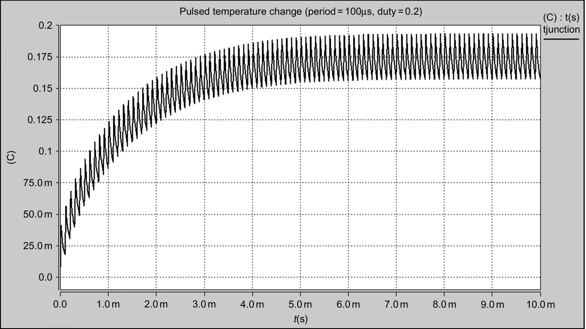
When the heat source pulse period is reduced to 100 μs (i.e., 10 kHz), the ripple on the temperature reduces significantly (Fig. 46.18).
One of the limitations with the ladder network is that it will tend to underestimate the thermal impedance for higher duty ratios, and while it is certainly very useful, it must be used with caution. It is possible to increase the accuracy by increasing the number of thermal RC stages; however, obviously, there will be a price to pay in terms of simulation speed as a result.
It is also very useful to note that the thermal models can be linked directly to the electric simulations with the power electronics, either using electric analogy models (i.e., electric resistance to represent thermal resistance) or more commonly in modern multiple-domain simulators directly as thermal models. It is, however, true to say that in most cases, the time constants of the thermal circuits are much longer than the switching periods of the power electronics and the user should therefore be prepared for running long simulations to achieve the steady-state temperature changes. Nevertheless, it can be extremely illuminating and helpful in understanding the true thermal state of the power electronics.
46.15 Summary
Thermal properties of devices, packages, and heat sinks can be modeled in a relatively simple and efficient manner using a number of simple lumped-model techniques. While this gives a good starting point for estimating the thermal impact on circuit performance, it is clearly a complex and interlinked area that requires detailed analysis to gain highly accurate solutions. However, the use of such models can help the designer gain an insight as to the effect of temperature on device and circuit behavior and as a result can profoundly improve the ultimate design. If the designer takes a “worst-case-scenario” approach to modeling thermal behavior, then they greatly increase their chances of obtaining a robust and efficient design that can cope with extremes of temperature in the environment or due to the device behavior.