
DSP-Based Control of Variable Speed Drives
Hamid A. Toliyat Texas A&M University, College Station, TX, United States
Mehdi Abolhassani Black & Decker (US) Inc., Towson, MD, United States
Peyman Niazi Maxtor Co., Shrewsbury, MA, United States
Lei Hao Wavecrest Laboratories, Rochester Hills, MI, United States
Abstract
High-performance motor drives are characterized by the need for smooth rotation down to stall, full control of torque at stall, and fast accelerations and decelerations. In the past, variable speed drives employed predominantly dc motors because of their excellent controllability. However, modern high-performance motor drive systems are usually based on three-phase ac motors, such as the ac induction motor or the permanent-magnet synchronous motor. These machines have supplanted the dc motor as the machine of choice for variety of applications because of their simple robust construction, low inertia, high power density, high torque density, and good performance at high speeds of rotation.
Keywords:
PI regulator; BLDC motor; PMSM; PMAC; A/D conversion
39.1 Introduction
High-performance motor drives are characterized by the need for smooth rotation down to stall, full control of torque at stall, and fast accelerations and decelerations. In the past, variable speed drives employed predominantly dc motors because of their excellent controllability. However, modern high-performance motor drive systems are usually based on three-phase ac motors, such as the ac induction motor (ACIM) or the permanent-magnet synchronous motor (PMSM). These machines have supplanted the dc motor as the machine of choice for variety of applications because of their simple robust construction, low inertia, high power density, high torque density, and good performance at high speeds of rotation.
The vector-control techniques are established for controlling these ac motors, and most modern high-performance drives now implement digital closed-loop current control. In such systems, the achievable closed-loop bandwidths are directly related to the rate at which the computationally intensive vector-control algorithms and associated vector rotations can be implemented in real time. Because of this computational burden, many high-performance drives now use digital signal processors (DSPs) to implement the embedded motor- and vector-control schemes. The DSPs are special microprocessors used where real-time manipulation of large amounts of digital data is required in order to implement complicated control algorithms. The inherent computational power of the DSP permits very fast cycle times and closed-loop current control bandwidths to be achieved.
The complete current control scheme for these machines also requires a high-precision pulse-width modulation (PWM) voltage-generation scheme and high-resolution analog-to-digital (A/D) conversion (ADC) for the measurement of the motor currents. In order to maintain a smooth control of torque to zero speed, rotor position feedback is essential for modern vector controllers. Therefore, many systems include rotor-position transducers, such as resolvers and incremental encoders.
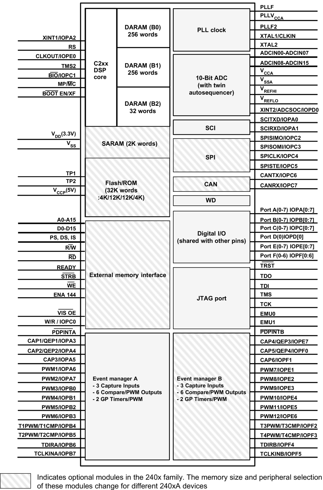
The Texas Instruments TMS320LF2407 DSP Controller (referred to as the LF2407 in this chapter) is a programmable digital controller with a C2xx DSP central processing unit (CPU) as the core processor. The LF2407 contains the DSP core processor and useful peripherals integrated onto a single piece of silicon. The LF2407 combines the powerful CPU with on-chip memory and peripherals. With the DSP core and control-oriented peripherals integrated into a single chip, users can design very compact and cost-effective digital control systems.
The LF2407 DSP controller offers 40 million instructions per second (MIPS) performance. This high processing speed of the C2xx CPU allows users to compute parameters in real time rather than lookup approximations from tables stored in memory. This fast performance is well suited for processing control parameters in applications such as notch filters or sensorless motor-control algorithms where a large amount of calculations must be computed quickly.
While the “brain” of the LF2407 DSP is the C2xx core, the LF2407 contains several control-orientated peripherals on board (see Fig. 39.1). The peripherals on the LF2407 make virtually any digital control requirement possible. Their applications range from analog-to-digital conversion to pulse-width modulation (PWM) generation. Communication peripherals make possible the communication with external peripherals, personal computers, or other DSP processors. Below is a graphic listing of the different peripherals on board the LF2407 depicted in Fig. 39.1.
We describe here the fundamental principles behind the implementation of high-performance controllers for three-phase ac motors—combining an integrated DSP controller, LF2407, flexible PWM generation, high-resolution A/D conversion, and embedded encoder interface.
39.2 Variable Speed Control of AC Machines
Efficient variable speed control of three-phase ac machines requires the generation of a balanced three-phase set of variable voltages with variable frequency. The variable-frequency supply is typically produced by conversion from dc using power semiconductor devices (typically MOSFETs or IGBTs) as solid-state switches. A commonly used converter configuration is shown in Fig. 39.2A. It is a two-stage circuit, in which the fixed-frequency 50 or 60 Hz ac supply is first rectified to provide the dc-link voltage, Vd, stored in the dc-link capacitor. This voltage is then supplied to an inverter circuit that generates the variable-frequency ac power for the motor. The power switches in the inverter circuit permit the motor terminals to be connected to either Vd or ground.
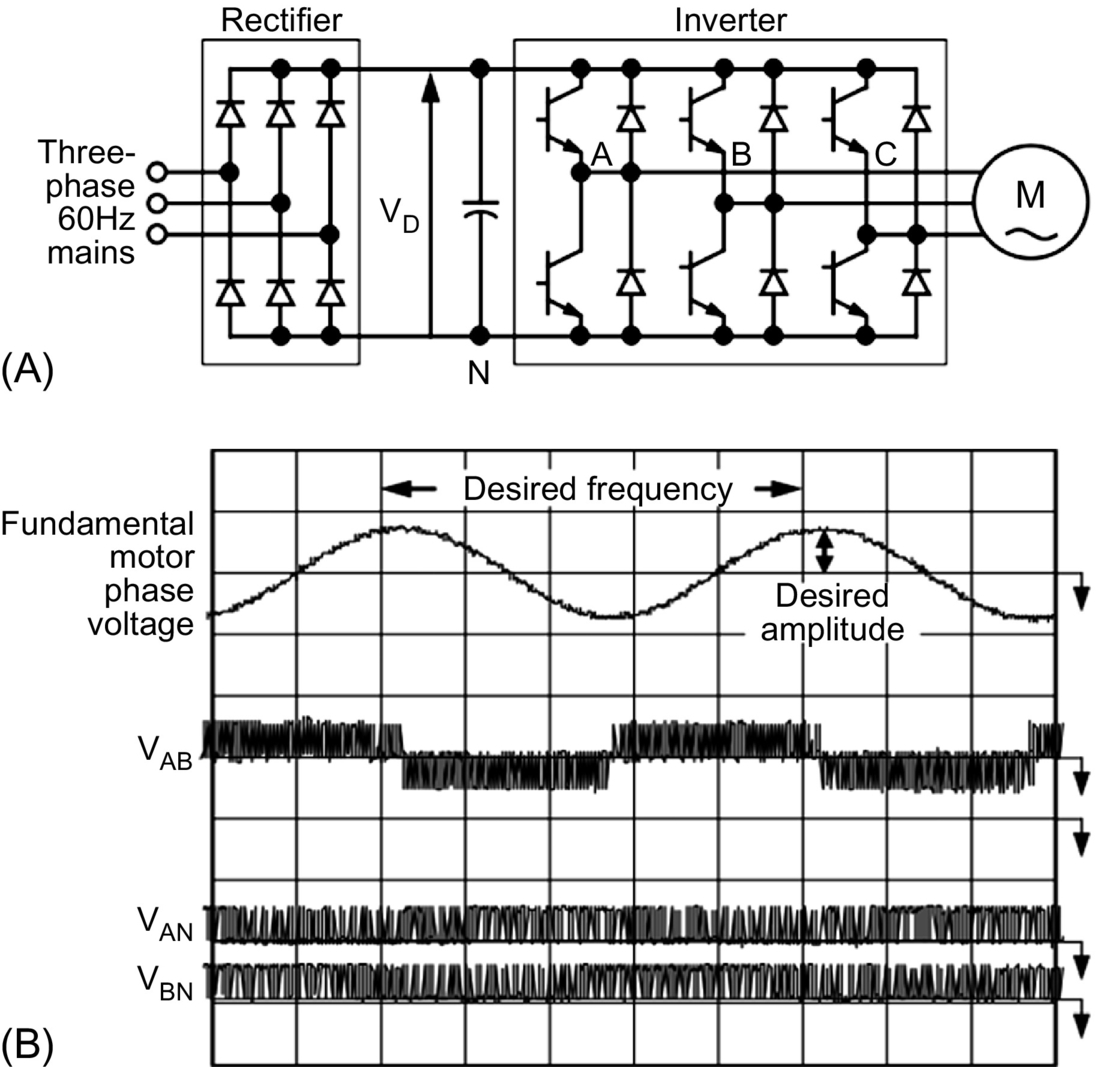
This mode of operation gives high efficiency because, ideally, the switch has zero loss in both the open and closed positions. By rapid sequential opening and closing of the six switches (Fig. 39.2A), a three-phase ac voltage with an average sinusoidal waveform can be synthesized at the output terminals. The actual output voltage waveform is a pulse-width modulated (PWM) high-frequency waveform, as shown in Fig. 39.2B. In practical, inverter circuits using solid-state switches and high-speed switching of about 20 kHz are possible. Therefore, sophisticated PWM waveforms with fundamental frequencies, nominally in the range of 0–250 Hz, can be generated. The inductive reactance of the motor increases with frequency. Thus, higher-order harmonic currents are very small, and near-sinusoidal currents flow in the stator windings. The fundamental voltage and output frequency of the inverter, as indicated in Fig. 39.2B, are adjusted by changing the PWM waveform using an appropriate controller. When controlling the fundamental output voltage, the PWM process inevitably modifies the harmonic content of the output voltage waveform. A proper choice of modulation strategy can minimize these harmonic voltages and, in result, harmonic losses in the motor.
39.3 General Structure of a Three-Phase AC Motor Controller
Accurate control of any motor drive process may ultimately be reduced to the problem of accurate control of both the torque and speed of the motor. In general, motor speed is controlled directly by measuring the motor's speed or position using appropriate transducers, and torque is controlled indirectly by suitable control of the motor phase currents. Fig. 39.3 shows a block diagram of a typical synchronous frame current controller for a three-phase motor. The figure also shows the proportioning of tasks between software code modules and the dedicated motor-control peripherals of a motor controller such as the LF2407. The controller consists of two proportional-plus-integral-plus-differential (PID) current regulators that are used to control the motor current vector in a reference frame that rotates synchronously with the measured rotor position.
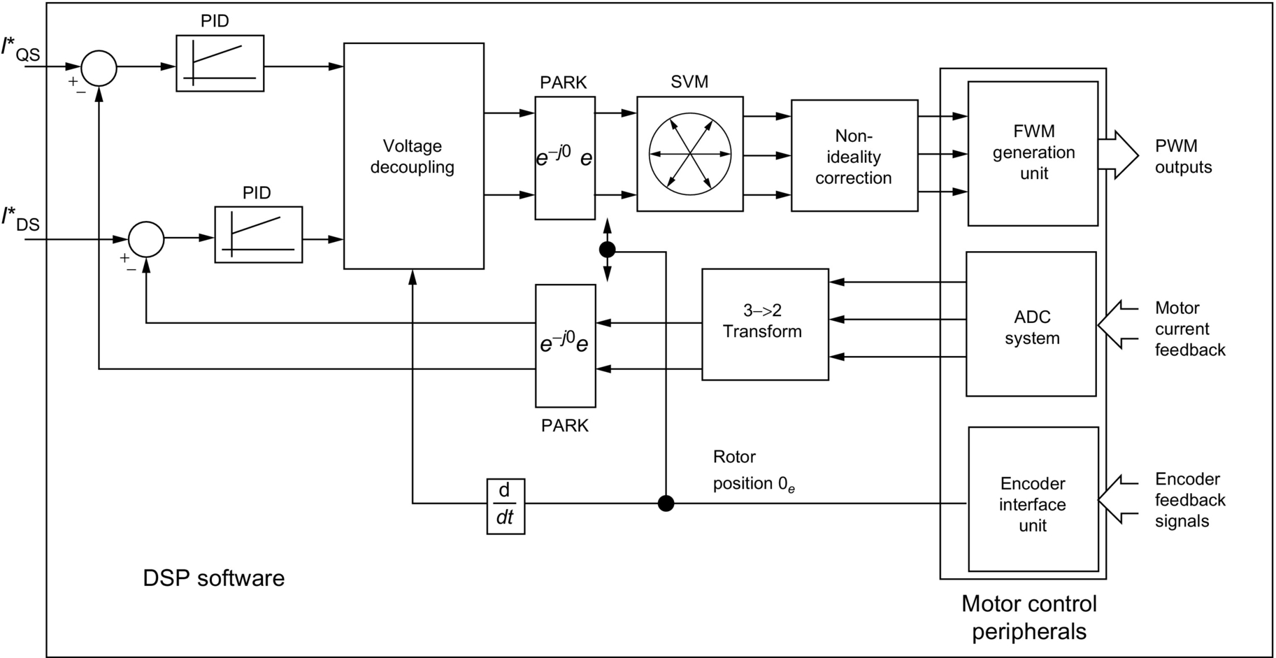
Sometimes, it may be desirable to implement a decoupling between voltage and speed that removes the speed dependencies and associated axes cross coupling from the control loop. The reference voltage components are then synthesized on the inverter using a suitable PWM strategy, such as space-vector modulation (SVM). It is also possible to incorporate some compensation schemes to overcome the distorting effects of the inverter switching dead time, finite inverter device on-state voltages, and dc-link voltage ripple. The two components of the stator current vector are known as the direct-axis and quadrature-axis components. The direct-axis current controls the motor flux and is usually controlled to be zero with permanent-magnet machines. The motor torque may then be controlled directly by regulation of the quadrature-axis component. Fast, accurate torque control is essential for high-performance drives in order to ensure rapid acceleration and deceleration and smooth rotation down to zero speed under all load conditions.
The actual direct and quadrature current components are obtained by first measuring the motor phase currents with suitable current-sensing transducers and converting them to digital, using an on-chip ADC system. It is usually sufficient to simultaneously sample just two of the motor line currents: since the sum of the three currents is zero, the third current can, when necessary, be deduced from simultaneous measurements of the other two currents. The controller software makes use of mathematical vector transformations, known as Park transformations that ensure that the three-phase set of currents applied to the motor is synchronized to the actual rotation of the motor shaft, under all operating conditions. This synchronism ensures that the motor always produces the optimal torque per ampere—that is, operates at optimal efficiency. The vector rotations require real-time calculation of the sine and cosine of the measured rotor angle, plus a number of multiply-and-accumulate operations. The overall control-loop bandwidth depends on the speed of implementation of the closed-loop control calculations and the resulting computation of new duty-cycle values. The inherent fast computational capability of the 40 MIPS, 16-bit fixed-point DSP core makes it the ideal computational engine for these embedded motor-control applications.
39.3.1 Pulse Width Modulation Generation
In typical ac motor-controller design, both hardware and software considerations are involved in the process of generating the PWM signals that are ultimately used to turn on or off the power devices in the three-phase inverter. In typical digital control environments, the controller generates a regularly timed interrupt at the PWM switching frequency (nominally 10–20 kHz). In the interrupt service routine, the controller software computes new duty-cycle values for the PWM signals used to drive each of the three legs of the inverter. The computed duty cycles depend on both the measured state of the motor (torque and speed) and the desired operating state. The duty cycles are adjusted on a cycle-by-cycle basis in order to make the actual operating state of the motor follow the desired trajectory.
Once the desired duty-cycle values have been computed by the processor, a dedicated hardware PWM generator is needed to ensure that the PWM signals are produced over the next PWM and controller cycle. The PWM generation unit typically consists of an appropriate number of timers and comparators that are capable of producing very accurately timed signals. Typically, 10- to 12-bit performance in the generation of the PWM timing waveforms is desirable.
Fig. 39.4 shows a typical PWM waveform for a single-leg inverter. In general, there is a small delay required between turning off one power device like A-phase lower device and turning on the complementary power device A-phase upper device. This dead time is required to ensure that the device being turned off has sufficient time to regain its blocking capability before the other device is turned on. Otherwise, a short circuit of the dc voltage could result.
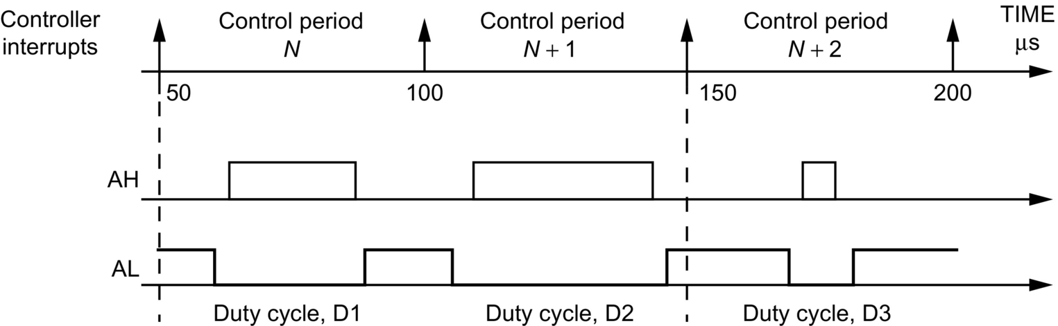
In LF2407, the compare units have been used to generate the PWM signals. The PWM output signal is high when the output of current PI regulation matches the value of T1CNT and is set to low when the timer underflow occurs. The switch states are controlled by the ACTR register. In order to minimize the switching losses, the lower switches are always kept on, and the upper switches are chopped on/off to regulate the phase current.
39.3.2 Analog-to-Digital Conversion Requirements
For the control of high-performance motor drives, fast, high-accuracy, simultaneous-sampling A/D conversion of the measured current values is required. The drives have a rated operation range—a certain power level that they can sustain continuously, with an acceptable temperature rise in the motor and power converter. They also have a peak rating—the ability to handle a current far in excess of the rated current for short periods of time. This allows a large torque to be applied transiently, to accelerate or decelerate the drive very quickly, and then to revert to the continuous range for normal operation. This also means that in the normal operating mode of the drive, only a small percentage of the total input range is being used.
At the other end of the scale, in order to achieve the smooth and accurate rotations desired in these machines, it is wise to compensate for small offsets and nonlinearities such as core saturation and parameter detuning. In any current-sensor electronics, the analog signal processing is often subject to gain and offset errors. Gain mismatches, for example, can exist between the current-measuring systems for different windings. These effects combine to produce undesirable oscillations in the torque. To meet both of these conflicting resolution requirements, modern motor drives use 10-bit A/D converters, depending on the cost/performance trade-off required by the application.
The bandwidth of the system is essentially limited by the amount of time it takes to input information and then perform the calculations. The A/D converters that take many microseconds to convert can produce intolerable delays in the system. A delay in a closed-loop system will degrade the achievable bandwidth of the system, and bandwidth is one of the most important figures of merit in these high-performance drives. Therefore, fast analog-to-digital conversion is a necessity for these applications.
A third important characteristic of the A/D converter used in these applications is timing. In addition to high resolution and fast conversion, simultaneous sampling is needed. In any three-phase motor, it is necessary to measure the currents in the three windings of the motor at exactly the same time in order to get an instantaneous “snapshot” of the torque in the machine. Any time skew (time delay between the measurements of the different currents) is an error factor that is artificially inserted by the means of measurement. Such a nonideality translates directly into a ripple of the torque—a very undesirable characteristic.
The analog-to-digital converter (ADC) on the LF2407 allows the DSP to sample analog or “real-world” voltage signals. The output of the ADC is an integer number that represents the voltage level sampled. The integer number may be used for calculations in an algorithm. The resolution of the ADC is 10 bits, meaning that the ADC will generate a 10-bit number for every conversion it performs. However, the ADC stores the conversion results in registers that are 16-bit wide. The 10 most significant bits are the ADC result, while the least significant bits (LSBs) are filled with “0”s. There are a total of 16 input channels to the single input ADC. The control logic of the ADC consists of autosequencers, which control the sampling of the 16 input channels to the ADC. The autosequencers control not only which channels (input channels) will be sampled by the ADC but also the order of the channels that the ADC performs conversions on. The two 8-conversion autosequencers can operate independently or cascade together as a “virtual” 16-conversion ADC.
39.3.3 Position Sensing and Encoder Interface Units
Usually, the motor position is measured through the use of an encoder mounted on the rotor shaft. The incremental encoder produces a pair of quadrature outputs (A and B), each with a large number of pulses per revolution of the motor shaft. For a typical encoder with 1024 lines, both signals produce 1024 pulses per revolution. Using a dedicated quadrature counter, it is possible to count both the rising and falling edges of both the A and B signals so that one revolution of the rotor shaft may be divided into 4096 different values. In other words, a 1024-line encoder allows the measurement of rotor position to 12-bit resolution. The direction of rotation may also be inferred from the relative phasing of quadrature signals A and B.
Fig. 39.5 shows the structure of an encoder. It consists of a light source, a radially slotted disk, and the photoelectric sensors. The disk rotates with the rotor. The two photosensors detect the light passing through the slots in the disk. When the light is hidden, a logic “0” is generated by the sensors. When the light passes through the slots of the disk, a logic “1” is produced. These logic signals are shown in Fig. 39.5. By counting the number of pulses, the motor speed can be calculated. The direction of rotation can be determined by detecting the leading signal between signals A and B.

This is all very well, but there is an increasing class of cost-sensitive motor drive applications with lower performance demands that can afford neither the cost nor the space requirements of the rotor position transducer. In these cases, the same motor-control algorithms can be implemented with estimated rather than measured rotor position.
The DSP core is quite capable of computing rotor position using sophisticated rotor-position estimation algorithms, such as extended Kalman estimators that extract estimates of the rotor position from measurements of the motor voltages and currents. These estimators rely on the real-time computation of a sufficiently accurate model of the motor in the DSP. In general, these sensorless algorithms can be made to work and the sensored algorithms at medium to high speeds of rotation. But as the speed of the motor decreases, the extraction of reliable speed-dependent information from voltage and current measurements becomes more difficult. In general, sensorless motor control is applicable principally to applications such as compressors, fans, and pumps, where continuous operation at zero or low speeds is not required.
39.3.4 The PI Regulator
An electric drive based on the field-orientated control (FOC) needs two constants as control parameters, the torque component reference iqse* and the flux component reference idse*. The classical PI regulator is well suited to regulate the torque and flux feedback to the desired values. This is because it is able to reach constant references by correctly setting both the proportional term (Kp) and the integral term (Ki), which are, respectively, responsible for the error sensibility and for the steady-state error. The numerical expression of the PI regulatoris as follows:

which is represented in Fig. 39.6.
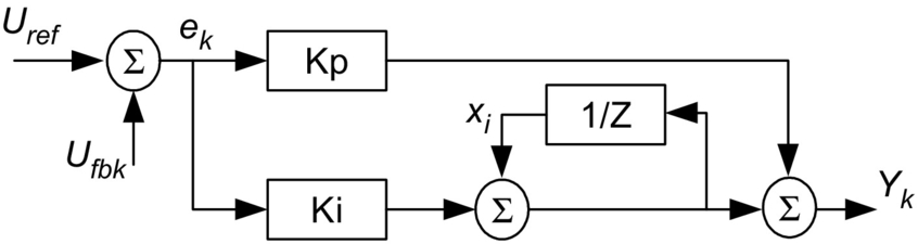
During normal operation, large reference value variations or disturbances may occur that result in the saturation and overflow of the regulator variables and output. To solve this problem, one solution is to add a correction of the integral component as depicted in Fig. 39.7.

The constants Kp, Ki, and Kc, proportional, integral, and integral correction components, respectively, are selected based on the sampling period and on the motor parameters. After defining the DSP-controlled motor drive requirements, in the following, we describe the digital control algorithms for permanent-magnet motors and induction motors.
39.4 DSP-Based Control of Permanent Magnet Brushless DC Machines
Permanent-magnet alternating current (PMAC) motors are synchronous motors that have permanent magnets mounted on the rotor and polyphase, usually three-phase, armature windings located on the stator. Since the field is provided by the permanent magnets, the PMAC motor has higher efficiency than induction- or switched-reluctance motors. The advantages of PMAC motors, combined with a rapidly decreasing cost of permanent magnets, have led to their widespread use in many variable speed drives such as robotic actuators, computer disk drives, appliances, automotive applications, and air-conditioning (HVAC) equipment.
In general, PMAC motors are categorized into two types. The first type of motor is referred to as PM synchronous motor (PMSM). These motors produce a sinusoidal back EMF, shown in Fig. 39.8A, and should be supplied with sinusoidal current/voltage. The PMSM's electronic control and drive system uses continuous rotor position feedback and PWM to supply the motor with the sinusoidal voltage or current. With this, constant torque is produced with very little ripple.
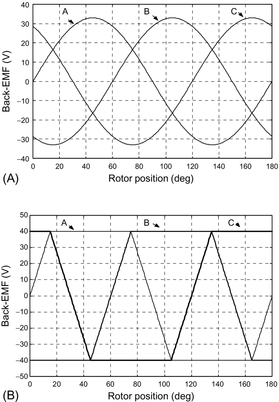
The second type of PMAC motor has a trapezoidal back EMF and is referred to as the brushless DC (BLDC) motor. The back EMF of the BLDC motor is shown in Fig. 39.8B. The BLDC motor requires that quasi-rectangular-shaped currents are fed into the machine. Alternatively, the voltage may be applied to the motor every 120 degrees, with a current limit to hold the currents within the motor's capabilities.
39.4.1 Mathematical Model of the BLDC Motor
The phase variables are used to model the BLDC motor due to its nonsinusoidal back EMF and phase current. The terminal voltage equation of the BLDC motor can be written as

where va, vb, and vc are the phase voltages; ia, ib, and ic are the phase currents; ea, eb, and ec are the phase back-EMF voltages; R is the phase resistance; Ls is the synchronous inductance per phase and includes both leakage and armature reaction inductances; and p represents d/dt. The electromagnetic torque is given by

where ωm is the mechanical speed of the rotor. The equation of motion is
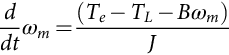
where TL is the load torque, B is the damping constant, and J is the moment of inertia of the rotor shaft and the load.
39.4.2 Torque Generation
From Eq. (39.3), the electromagnetic torque of the BLDC motor is related to the product of the phase back EMF and current. The back EMFs in each phase are trapezoidal in shape and are displaced by 120 electrical degrees with respect to each other in a three-phase machine. A rectangular current pulse is injected into each phase so that current coincides with the crest of the back-EMF waveform; hence, the motor develops an almost constant torque. This strategy, commonly called six-step current control, is shown Fig. 39.9. The amplitude of each phase's back EMF is proportional to the rotor speed and is given by

where k is a constant and depends on the number of turns in each phase, φ is the permanent-magnet flux, and ωm is the mechanical speed. In Fig. 39.9, during any 120 degrees interval, the instantaneous power converted from electric to mechanical, Po, is the sum of the contributions from two phases in series and is given by
where Te is the output torque and I is the amplitude of the phase current. From Eqs. (39.4) and (39.6), the expression for output torque can be written as
where Kt is the torque constant. Since the electromagnetic torque is only proportional to the amplitude of the phase current in Eq. (39.7), torque control of the BLDC motor is essentially accomplished by phase current control.
39.4.3 BLDC Motor Control Topology
Based on the previously discussed concept, a BLDC motor drive system is shown in Fig. 39.10. It can be seen that the total drive system consists of the BLDC motor, power electronic converter, sensor, and controller.

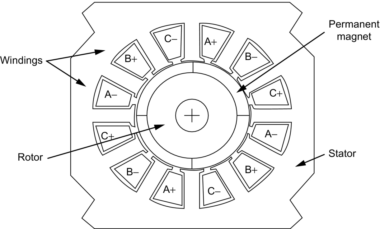
The BLDC motors are predominantly surface-magnet machines with wide magnet pole arcs. The stator windings are usually concentrated windings, which produce a square waveform distribution of flux density around the air gap. The design of the BLDC motor is based on the crest of each half cycle of the back-EMF waveform. In order to obtain a smooth output torque, the back-EMF waveform should be wider than 120 degrees electrical degrees. A typical BLDC motor with 12 stator slots and 4 poles on the rotor is shown in Fig. 39.11. The inverter is usually responsible for the electronic commutation and current regulation. For the six-step current control, if the motor windings are Y-connected without the neutral connection, only two of the three-phase currents flow through the inverter in series. This results in the amplitude of the DC-link current always being equal to that of the phase currents. The PWM current controllers are typically used to regulate the actual machine currents in order to match the rectangular current reference waveforms shown in Fig. 39.9. For example, during one 60 degrees interval, when switches T1 and T6 are active, phases A and B conduct. The lower switch T6 is always turned on, and the upper switch T1 is chopped on/off using either a hysteresis current controller with variable switch frequency or a PI controller with fixed switch frequency.
When T1 and T6 are conducting, current builds up in the path as shown in Fig. 39.12A with dashed line. When switch T1 is turned off, the current decays through diode D4 and switch T6 as depicted in Fig. 39.12B. In the next interval, switch T2 is on, and T1 is chopped so that phase A and phase C conduct. During the commutation interval, the phase-B current rapidly decreases through the freewheeling diode D3 until it becomes zero and the phase C current builds up.

From the above analysis, each of the upper switches is always chopped for one 120 degrees interval, and the corresponding lower switch is always turned on per interval. The freewheeling diodes provide the necessary paths for the currents to circulate when the switches are turned off and during the commutation intervals. There are two types of sensors for the BLDC drive system: a current sensor and a position sensor. Since the amplitude of the dc-link current is always equal to the motor phase current in six-step current control, the dc-link current is measured instead of the phase current. Thus, a shunt resistor, which is in series with the inverter, is usually used as the current sensor. Hall-effect position sensors typically provide the position information needed to synchronize the stator excitation with rotor position in order to produce constant torque. Hall-effect sensors detect the change in magnetic field. The rotor magnets are used as triggers for the Hall sensors. A signal-conditioning circuit is needed for noise cancellation in Hall-effect sensor circuits. In six-step current control algorithm, rotor position needs to be detected at only six discrete points in each electric cycle. The controller tracks these six points so that the proper switches are turned on or off for the correct intervals. Three Hall-effect sensors, spaced 120 electrical degrees apart, are mounted on the stator frame. The digital signals from the Hall sensors are then used to determine the rotor position and switch gating signals for the inverter switches.
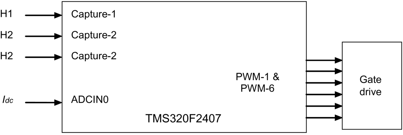
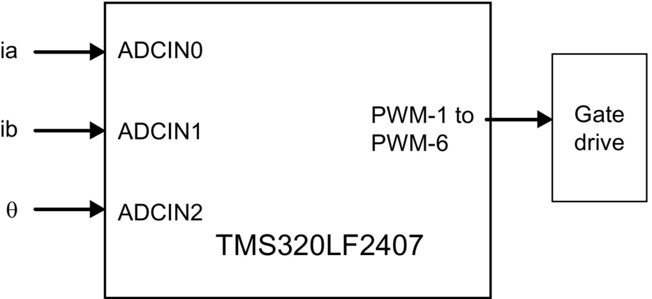
39.4.4 DSP Controller Requirements
The controller of BLDC drive systems reads the current and position feedback, implements the speed or torque control algorithm, and finally generates the gate signals. The connectivity of the LF2407 in this application is illustrated in Fig. 39.13. Three capture units in the LF2407 are used to detect both the rising and falling edges of Hall-effect signals. Hence, in every 60 electrical degrees of motor rotation, one capture unit interrupt is generated that ultimately causes a change in the gating signals and the motor to move to the next position. One input channel of the 10-bit A/D converter reads the dc-link current. The output pins PWM1–PWM6 are used to supply the gating signals to the inverter.
39.4.5 Implementation of the BLDC Motor Control Algorithm Using LF2407
A block diagram of the BLDC motor-control system is shown in Fig. 39.14. The dashed line separates the software from the hardware components introduced in the previous section. It is necessary to choose hardware components carefully in order to ensure high processing speed and precision in the overall control system. The overall control algorithm of the BLDC motor consists of nine modules:

• Detection of Hall-effect signals
• Speed control subroutine
• Measurement of current
• Speed profiling
• Calculation of actual speed
• PID regulation
• PWM generation
• DAC output
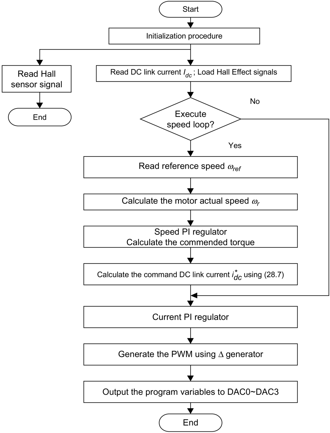
The flowchart of the overall control algorithm is illustrated in Fig. 39.15.
39.5 DSP-Based Control of Permanent Magnet Synchronous Machines
As previously described, the permanent-magnet synchronous motor (PMSM) is a PM motor with a sinusoidal back EMF. Compared with the BLDC motor, it has less torque ripple because the torque pulsations associated with current commutation do not exist. A carefully designed machine in combination with a good control technique can yield a very low level of torque ripple (<2% rated), which is attractive for high-performance motor-control applications such as machine tool and servo applications.
In this section, following the same procedures used in the previous section, the principles of the PMSM drive system will be introduced. Later, the control implementation using the LF2407 DSP will be described in detail.
39.5.1 Mathematical Model of PMSM
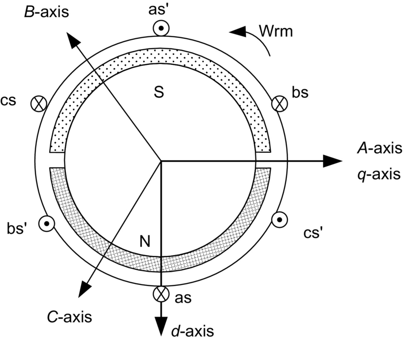
Fig. 39.16 depicts the simplified three-phase surface-mounted PMSM motor for our discussion. The stator windings, as-as′, bs-bs′, and cs-cs′, are shown as lumped windings for simplicity but are actually distributed around the stator. The rotor has two poles. Mechanical rotor speed and position are denoted as ωrm and θrm, respectively. Electric rotor speed and position, ωr and θr, are defined as P/2 times the corresponding mechanical quantities, where P is the number of poles.
Based on the above motor definition, the voltage equation in the abc stationary reference frame is given by

where
and the stator resistance matrix is given by
The flux linkages equation can be expressed by
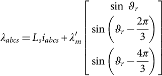
where λ′m denotes the amplitude of the flux linkages established by the permanent magnet as viewed from the stator phase windings. Note that in Eq. (39.11), the back EMFs are sinusoidal waveforms that are 120 degrees apart from each other.
The stator self-inductance matrix, Ls, is given as
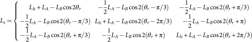
The electromagnetic torque may be written as
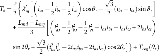
In Eq. (39.13), Tcog (θr) represents the cogging torque, and the d- and q-axes magnetizing inductances are defined by
and
The torque and speed are related by the electromechanical motion equation
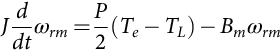
where J is the rotational inertia, Bm is the approximated mechanical damping due to friction, and TL is the load torque.
39.5.2 Mathematical Model of PMSM in Rotor Reference Frame
The voltage and torque equations can be expressed in the rotor reference frame in order to transform the time-varying variables into steady-state constants. The transformation of the three-phase variables in the stationary reference frame to the rotor reference frame is defined as
where
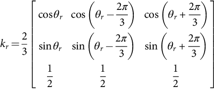
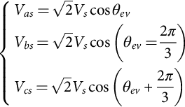
If the applied stator voltages are given by
then applying Eq. (39.16) to Eqs. (39.8), (39.11), and (39.17) yields
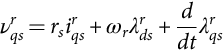
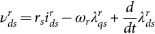
where the q- and d-axes self-inductances are given by Lqs=Lls+Lmq and Lds=Lls+Lmd, respectively.
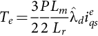
The electromagnetic torque can be written as
From Eq. (39.22), it can be seen that torque is related only to the d- and q-axes currents. Since Lq≥Ld (for surface-mounted PMSM, both inductances are equal), the second item contributes a negative torque if the flux-weakening control has been used. In order to achieve the maximum torque/current ratio, the d-axis current is set to zero during the constant torque control so that the torque is proportional only to the q-axis current. Hence, this results in the control of the q-axis current for regulating the torque in rotor reference frame.
39.5.3 PMSM Control Topology
Based on the above analysis, a PMSM drive system is developed as shown in Fig. 39.17. The total drive system looks similar to that of the BLDC motor and consists of a PMSM, power electronic converter, sensors, and controller. These components are discussed in detail in the following sections.

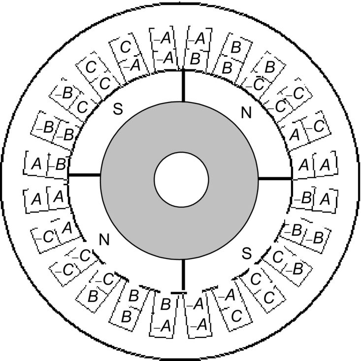
The design consideration of the PMSM is to first generate the sinusoidal back EMF. Unlike the BLDC, which needs concentrated windings to produce the trapezoidal back EMF, the stator windings of PMSM are distributed in as many slots per pole as deemed practical to approximate a sinusoidal distribution. To reduce the torque ripple, standard techniques such as skewing and chorded windings are applied to the PMSM. With the sinusoidally excited stator, the rotor design of the PMSM becomes more flexible than the BLDC motor where the surface-mounted permanent magnet is a favorite choice. Besides the common surface-mounted nonsalient pole PM rotor, the salient pole rotors, like inset and buried magnet rotors, are often used because they offer appealing performance characteristics during the flux-weakening region. A typical PMSM with 36 stator slots in stator and 4 poles on the rotor is shown in Fig. 39.18.
Due to the sinusoidal nature of the PMSM, control algorithms such as V/f and vector control, developed for other AC motors, can be directly applied to the PMSM control system. If the motor windings are Y-connected without a neutral connection, three-phase currents can flow through the inverter at any moment. With respect to the inverter switches, three switches, one upper and two lower in three different legs, conduct at any moment as shown in Fig. 39.19. The PWM current control is still used to regulate the actual machine current. Either a hysteresis current controller, a PI controller with sine triangle, or an SVPWM strategy is employed for this purpose. Unlike the BLDC motor, the three switches are switched at any time.

39.5.4 DSP Controller Requirements
The LF2407 is used as the controller to implement speed control of the PMSM system. The interface of the LF2407 is illustrated in Fig. 39.20. Similar to the BLDC motor-control system, three input channels are selected to read the two-phase currents and resolver signal. Because a resolver is used in one case, the quadrature-encoder-pulse (QEP) inputs are not used. The QEP inputs work only with a QEP signal that a rotary encoder supplies. The DSP output pins PWM1–PWM6 are used to supply the gating signals to the switches and form the output of the control part of the system.
39.5.5 Implementation of the PMSM Algorithm Using the LF2407
The block diagram of the PMSM drive system is displayed in Fig. 39.21.
The flowchart of the developed software is shown in Fig. 39.22. The control program of the PMSM has one main routine and includes four modules:

• DAC module
• ADC module
• Speed control module
In the following section, speed control module is discussed.
39.5.5.1 The Speed Control Algorithm
The requirement for speed control algorithm can be itemized as follows:
• Reading the current and position signal and then generating the commanded speed profile
• Calculating the actual motor speed and transferring the variables in the abc model to the d-q model and reverse
• Regulating the motor speed and currents using the vector-control strategy
• Generating the PWM signal based on the calculated motor phase voltages
The PWM frequency is determined by the time interval of the interrupt, with the controlled phase voltages being recalculated every interrupt.
39.6 DSP-Based Vector Control of Induction Motors
For many years, induction motors have been preferred for a variety of industrial applications because of their robust and rugged construction. Compared to dc motors, induction motors are not as easy to control. They typically draw large starting currents, about six to eight times their full-load values, and operate with lagging power factor when loaded. However, with the advent of the vector-control concept for motor control, it is possible to decouple the torque and the flux, thus making the control of the induction motor very similar to that of the dc motor.
The most popular type of induction motor used is the squirrel-cage induction motor. The rotor consists of a laminated core with parallel slots for carrying the rotor conductors, which are usually heavy bars of copper, aluminum, or alloys. One bar is placed in each slot, or rather, the bars are inserted from the end when the semiclosed slots are used. The rotor bars are brazed, electrically welded, or bolted to two heavy and stout short-circuiting end rings, thus completing the squirrel-cage construction. The rotor bars are permanently short-circuited on themselves. The rotor slots are usually not parallel to the shaft but are given a slight angle, called a skew, which increases the rotor resistance due to increased length of rotor bars and an increase in the slip for a given torque. The skew is also advantageous because it reduces the magnetic hum while the motor is operating and reduces the locking tendency or cogging of the rotor teeth.
When the three-phase stator windings are fed by a three-phase supply, a magnetic flux of a constant magnitude rotating at synchronous speed is created in the air gap. Due to the relative speed between the rotating flux and the stationary conductors, an electromagnetic force (EMF) is induced in the rotor in accordance with Faraday's laws of electromagnetic induction. The frequency of the induced EMF is the same as the supply frequency, and the magnitude is proportional to the relative velocity between the flux and the conductors. Therefore, the rotor current develops in the same direction as the flux and tries to catch up with the rotating flux.
39.6.1 Induction Motor Field-oriented Control
The term “vector” control refers to the control technique that controls both the amplitude and the phase of ac excitation voltage. Vector control controls the spatial orientation of the EMF in the machine. This has led to the coining of the term FOC, which is used for controllers that maintain a 90 degrees spatial orientation between the critical field components.
The required 90 degrees of spatial orientation between key field components can be compared with the dc motor, where the armature winding magnetic field and the field winding magnetic field are always in quadrature. The objective is to force the control of the induction machine to be similar to the control of a dc motor, that is, torque control. In dc machines, the field and the armature winding axes are orthogonal to one another, making the magnetomotive forces (MMFs) established orthogonal. If the iron saturation is ignored, then the orthogonal fields can be considered to be completely decoupled.
It is important to maintain a constant field flux for proper torque control. It is also important to maintain an independently controlled armature current in order to overcome the effects of the detuning of resistance of the armature winding and leakage inductance. A spatial angle of 90 degrees between the flux and MMF axes has to be maintained in order to limit the interaction between the MMF and the flux. If these conditions are met at every instant of time, the torque will always follow the current.
With vector control, the mechanically robust induction motors can be used in high-performance applications where dc motors were previously used. The key feature of the control scheme is the orientation of the synchronously rotating q-d-0 frame to the rotor flux vector. The d-axis component is aligned with the rotor flux vector and regarded as the flux-producing current component. On the other hand, the q-axis current, which is perpendicular to the d-axis, is solely responsible for torque production.
In order to apply a rotor flux field-orientation condition, the rotor flux linkage is aligned with the d-axis, so the q-axis rotor flux in excitation reference frame λqre will be zero, and the d-axis rotor flux in the excitation reference frame will be the rotor flux, ![]() . Therefore, we have
. Therefore, we have

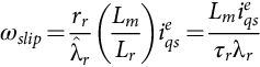
where τr is rotor time constant, Lm magnetizing inductance, Lr, rotor leakage inductance, rr, rotor resistance, iqse q-axis stator current in excitation frame, idse d-axis stator current in excitation frame, and ωslip angular frequency of slip. We can find out that in this case, idse controls the rotor flux linkage and iqse controls the electromagnetic torque. The reference currents of the q-d-0 axis (iqse*,idse*) are converted to the reference phase voltages (vdse*,vqse*) as the commanded voltages for the control loop. Given the position of the rotor flux and two-phase currents, this generic algorithm implements the instantaneous direct torque and flux control by means of coordinate transformations and PI regulators, thereby achieving accurate and efficient motor control.
It is clear that for implementing vector control, we have to determine the rotor flux position. This usually is performed by measuring the rotor position and utilizing the slip relation to compute the angle of the rotor flux relative to the rotor axis.
Equations (39.23) and (39.24) show that we can control torque and field by ids and iqs in the excitation frame. However, in the implementation of FOC, we need to know ids and iqs in the stationary reference frame. So, we have to know the angular position of the rotor flux to transform ids and iqs from the excitation frame to the stationary frame. By using ωslip, which is shown in Eq. (39.24), and using actual rotor speed, the rotor flux position is obtained:
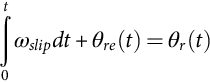
where θre(t) is electric angular rotor position and θr(t) angular rotor flux position.
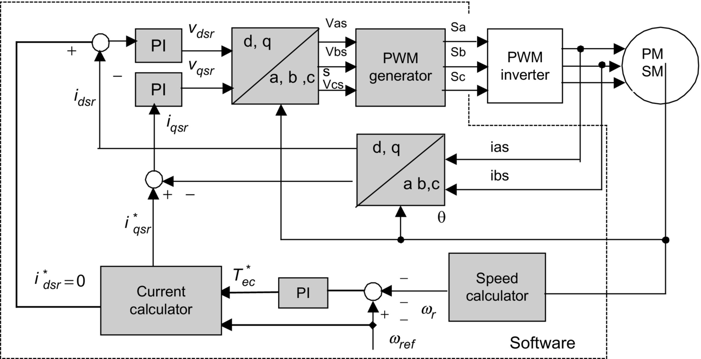
The current model takes ids and iqs as inputs and the rotor mechanical speed and gives the rotor flux position as an output. Fig. 39.23 shows the block diagram of the vector-control strategy in which speed regulation is possible using a control loop.
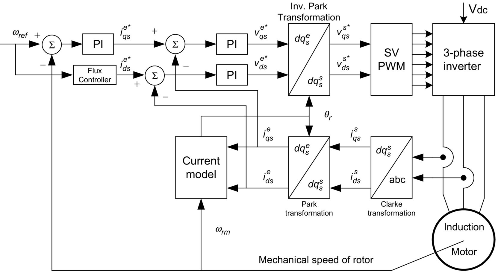
As shown in Fig. 39.23, two-phase currents are measured and fed to the Clarke transformation block. These projection outputs are indicated as idss and iqss. These two components of the current provide the inputs to Park's transformation, which gives the currents in the qdse excitation reference frame. The idse and iqse components, which are outputs of the Park transformation block, are compared with their reference values idse*, the flux reference, and iqse*, the torque reference. The torque command, iqse*, comes from the output of the speed controller. The flux command, idse*, is the output of the flux controller that indicates the right rotor flux command for every speed reference. For idse*, we can use the fact that the magnetizing current is usually between 40% and 60% of the nominal current. For operating in speeds above the nominal speed, a field-weakening section should be used in the flux controller section. The current regulator outputs, vdse* and vqse*, are applied to the inverse Park transformation. The outputs of this projection are vdse and vqss, which are the components of the stator voltage vector in the dqss orthogonal reference frame. They form the inputs of the space-vector PWM block. The outputs of this block are the signals that drive the inverter.
Note that both the Park and the inverse Park transformations require the exact rotor flux position, which is given by the current model block. This block needs the rotor resistance or rotor time constant as a parameter. Accurate knowledge of the rotor resistance is essential to achieve the highest possible efficiency from the control structure. The lack of this knowledge results in the detuning of the FOC. In Fig. 39.23, a space-vector PWM has been used to emulate vdss and vqss in order to implement current regulation.
39.6.2 DSP Controller Requirements
The controller of the induction motor-control system is used to read the feedback current and position signals, to implement the speed or torque control algorithm, and to generate the gate signals based on the control signal. Analog controllers or digital signal processors, such as LF2407, can perform these tasks.
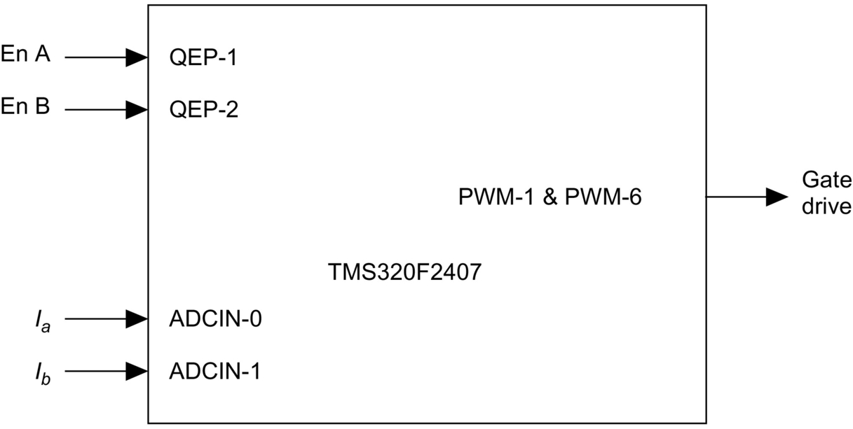
The interface of the LF2407 is illustrated in Fig. 39.24. Two quadrature counters detect the rising and falling edges of the encoder signals. Two input channels related to the 10-bit ADC are selected to read the two-phase currents. The pins PWM1–PWM6 output the gating signals to the gate drive circuitry.
39.6.3 Implementation of Field-Oriented Speed Control of Induction Motor
Some practical aspects of implementing the block diagram of Fig. 39.24 are discussed in this section and subsections. The software organization, the utilization of different variables, and the handling of the DSP controller resources are described. In addition, the control structure for the per-unit model is presented. Next, some numerical considerations have been made in order to address the problems inherent within the fixed-point calculation. As described, current model is one of the most important blocks in the block diagram depicted in Fig. 39.23. The inputs of this block are the currents and mechanical speed of rotor. In the next sections, technical points that should be considered during current and speed measurement and their scaling are discussed.
39.6.3.1 Software Organization
The body of the software consists of two main modules: the initialization module and the PWM interrupt service routine (ISR) module. The initialization model is executed only once at start-up. The PWM ISR module interrupts the waiting infinite loop when the timer underflows. When the underflow interrupt flag is set, the corresponding ISR is served. Fig. 39.25 shows the general structure of the software. The complete FOC algorithm is executed within the PWM ISR so that it runs at the same frequency as the switching frequency or at a fraction of it. The wait loop could be easily replaced with a user interface.

39.6.3.2 Base Values and Per-Unit Model
It is often convenient to express machine parameters and variables of per-unit quantities. Moreover, the LF2407 is a fixed-point DSP, so using a normalized per-unit model of the induction motor is easier than using real parameters. In this model, all quantities refer to the base values. Base power and base voltage are selected, and all parameters and variables are normalized using these base quantities. Although one might violate this convention from time to time when dealing with instantaneous quantities, the rms values of the rated phase voltage and current are generally selected as the base voltage for the a-b-c variables, while the peak value is generally selected as the base voltage for d-q variables. The base values are determined from the nominal values by using Eq. (39.27), where In, Vn, and fn are the nominal phase current, the nominal phase-to-neutral voltage, and the nominal frequency in a star-connected induction motor, respectively. The base value definitions are as follows:

where Ib and Vb are the maximum values of the nominal phase current and voltage, ωb is the electric nominal rotor flux speed, and ψb is the base flux.
39.6.3.3 Speed Estimation During High-Speed Region
As previously mentioned, this method is based on counting the number of encoder pulses in a specified time interval. The QEP assigned timer counts the number of pulses and records it in the timer counter register (TxCNT). As the mechanical time constant is much slower than the electric one, the speed regulation loop frequency might be lower than the current loop frequency. The speed regulation loop frequency is obtained in this algorithm by means of a software counter. This counter accepts the PWM interrupt as input clock, and its period is the software variable called SPEEDSTEP. The counter variable is named speedstep. When speedstep is equal to SPEEDSTEP, the number of pulses counted is stored in another variable called np, and thus, the speed can be calculated. The scheme depicted in Fig. 39.26 shows the structure of the speed feedback generator.

Assuming that np is the number of encoder pulses in one SPEEDSTEP period when the rotor turns at the nominal speed, a software constant Kspeed should be chosen as follows:
The speed feedback can then be transformed into a Q4.12 format, which can be used in the control software. In the proposed control system, the nominal speed is 1800 rpm, and SPEEDSTEP is set to 125. The np can be calculated as follows:
where ![]() (PWM frequency is 10 kHz, but the program is running at 3333 Hz) and hence Kspeed is given by
(PWM frequency is 10 kHz, but the program is running at 3333 Hz) and hence Kspeed is given by
Note that Kspeed is out of the Q4.12 format range. The most appropriate format to handle this constant is the Q8.8 format. The speed feedback in Q4.12 format is then obtained from the encoder by multiplying np by Kspeed. The flowchart of speed measurement is presented in Fig. 39.27.

39.6.3.4 Speed Measurement During Low-Speed Region
To detect the edges of two successive encoder pulses, the developed program can use either the QEP counter or the capture unit input pins. The program has to measure the time between two successive pulses; therefore, it must utilize another GP timer. In this program, timer 3 has been dedicated to the time measurement. During the interrupt service routine of the capture unit or counter QEP, speed can be calculated. To obtain the actual speed of the motor, the appropriate number is divided by the value in the count register of timer 3.
As it can be inferred, at very low speeds, an overflow may occur in timer 3. The counter would then reset itself to zero and start counting up again. This event results in a large error in speed measurement. To avoid this event, timer 3 will be disabled in the overflow interrupt service routine. However, this timer is enabled in the capture unit (counter QEP) interrupt.
The flowchart of this implementation is presented in Fig. 39.28.

39.6.3.5 The Current Model
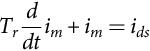
The current model is used to find the rotor flux position. This module takes ids and iqs as inputs plus the rotor electric speed and then calculates the rotor flux position. The current model is based on Eqs. (39.23) and (39.24). Eq. (39.23) in transient form can be written as

Assume λdr/Lm=im where im is the magnetizing current; therefore, Eq. (39.29) can be written as follows:
Rotor flux speed in a per-unit system can be shown by
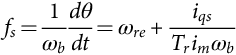
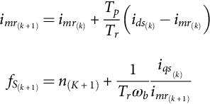
where θ is the rotor flux position and Tr=Lr/rr and ωre are the rotor time constant and rotor electric speed, respectively. The rotor time constant is critical to the correct functionality of the current model. This system outputs the rotor flux speed, which in turn will be integrated to get the rotor flux position. Assuming that ![]() , Eqs. (39.30) and (39.31) can be discretized as follows:
, Eqs. (39.30) and (39.31) can be discretized as follows:
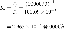
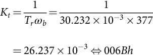
For example, let the constants Tp/Tr and 1/Trωb be renamed to Kt and Kt, respectively. Here, Lr=73.8 mH, rr=0.73 Ω, and fn=60 Hz. So for Kt and Kr, we have
By knowing the rotor flux speed (fs), the rotor flux position (θcm) is computed by the integration formula in the per-unit system:
In Eq. (39.33), let ωbfsT be called θinc. This variable is the rotor angle variation within one sampling period. Thus, the current model module has three input variables ids, ids, and ωre and one output, which is the rotor flux position θcm represented as a 16-bit integer value. The flowchart of the field-oriented speed control of induction motor is presented in Fig. 39.29. This routine is placed inside the PWM interrupt service routine.
