
Computer Simulation of Power Electronics and Motor Drives
Michael Giesselmann Texas Tech University, Lubbock, TX, United States
Abstract
This chapter shows how power electronics, electric motors, and drives can be simulated with modern spice-based software simulation tools. The focus will be on LTspice, which is widely used and available for free download for all contemporary (2016) Windows 7, 8, and 10 PCs. The LTspice examples have been developed for the current LTspice IV version of the software [1]. LTspice lends itself especially well to simulations of switch-mode power electronics circuits since it was designed to support Linear Technologies' family of products. This product line includes a large number of switch-mode power conversion parts. This manifests itself in the stability of the simulator during switching transitions. The author found the use of these examples is very beneficial in an educational environment, since the examples can be shared with students to enhance their understanding of the lecture material. The concepts and examples presented here can also be used for serious professional work. In fact, the author has used these tools with great success in many research projects. In addition to LTspice, PTC Mathcad [2] has been used to derive and present the underlying equations. Equations created in Mathcad look as perfect as in the best typesetting software, but they can also be evaluated numerically and manipulated symbolically to derive additional equations and to validate the underlying theory.
Keywords
Simulation of power electronics; Modeling of AC induction machines; Sensorless vector control; Induction motor control; Avoiding/mitigating convergence problems
44.1 Introduction
This chapter shows how power electronics, electric motors, and drives can be simulated with modern spice-based software simulation tools. The focus will be on LTspice, which is widely used and available for free download for all contemporary (2016) Windows 7, 8, and 10 PCs. The LTspice examples have been developed for the current LTspice IV version of the software [1]. LTspice lends itself especially well to simulations of switch-mode power electronics circuits since it was designed to support Linear Technologies' family of products. This product line includes a large number of switch-mode power conversion parts. This manifests itself in the stability of the simulator during switching transitions. The author found the use of these examples is very beneficial in an educational environment, since the examples can be shared with students to enhance their understanding of the lecture material. The concepts and examples presented here can also be used for serious professional work. In fact, the author has used these tools with great success in many research projects. In addition to LTspice, PTC Mathcad [2] has been used to derive and present the underlying equations. Equations created in Mathcad look as perfect as in the best typesetting software, but they can also be evaluated numerically and manipulated symbolically to derive additional equations and to validate the underlying theory.
The software examples have been developed to illustrate advanced techniques for the simulation of power electronics and motor drives but not to teach the basic features of LTspice. For that, the reader shall be referred to the online documentation [1]. In addition, it is assumed that the reader is familiar with the basics of power electronics and electric machines, specifically AC induction machines. For a review, the reader shall be referred to [3] for power electronics and [4,5] for induction machines.
44.2 Use of Simulation Tools for Design and Analysis
It is appropriate to reflect upon the value of simulations and its place in the design and analysis process before any in-depth discussion of specific simulation examples. Computer simulations enable engineers to study the behavior of complex and powerful systems without actually building or operating them. Simulations therefore have a place in the analysis of existing equipment and the design of new systems. In addition, computer simulations enable engineers to safely study high-power circuits including abnormal operating conditions without actually creating such conditions in a real environment.
However, even the most advanced simulation software cannot perfectly represent all effects in real hardware. The accuracy of the results depends on the accuracy of the component models and the proper identification and inclusion of parasitic circuit elements such as parasitic inductance, capacitance, and mutual coupling. Discrepancies between simulation and experimental results often occur if the underlying assumptions for the device model have been exceeded. For example, an attempt to model transformer inrush with a transformer model that assumes linear magnetics would not yield useful results.
In particular, the precise prediction of voltage and current traces during fast switching transitions in power electronics circuits has been proven to be difficult. To obtain useful results, extensive experimental validation, advanced device models (and the values for their parameters!), and detailed knowledge of parasitic elements, including the ones associated with the packaging of the circuit elements, are necessary. Therefore, the exact prediction of waveforms during switching transitions shall be excluded from the discussions in this chapter. Consequently, the author prefers to measure parameters such as voltage rise and fall times and over- and undershoot on actual circuitry in the laboratory.
Sometimes, users of spice-based simulators claim that the simulations of power electronics circuits with steep signal transitions are difficult due to convergence problems. However, with the proper techniques of gate signal generation, we can simulate just about any given circuit with little or no convergence problems in many spice-based tools. In addition, if convergence problems are avoided, simulations run much faster and larger numbers of individual transitions can be studied. This is achieved by generating gate signals using dependent sources with mathematical functions that produce switching signals that are differentiable throughout the transition. Being able to run simulations with a large number of transitions fast and without convergence problems gives a lot of insight into the cycle-by-cycle and the system level behavior of a power electronics circuit. An excellent application for these cycle-by-cycle simulations is the development and verification of control strategies for the power semiconductors in power electronics circuits.
Dependent voltage and current sources included in LTspice can be used to study large and complex systems like field-oriented (also called vector) control of induction machines if the proper mathematical control functions are used. Details are given below. In the examples for vector control of induction motors, the power electronics inverter is replaced with a dependent voltage source that represents the short-term average (filtering away the high-frequency voltage components associated with the switching frequency) of the output of a three-phase inverter. These examples represent system level simulations, which could have also been done using programs like MatLab/Simulink. However, circuit simulation software also provides the option of studying actual circuit level details in complex systems. To demonstrate this capability, the start-up of an induction motor, fed by a three-phase inverter with actual switch-mode operation, is presented.
In all modeling cases, the user needs to define the goal of the simulation effort. In other words, the user must answer the question “What information shall be obtained through the simulation of the circuit or system?” The user must then select the appropriate simulation software and the appropriate models. This process requires a detailed understanding of the properties and limitations of the device models and the sensitivity of the results to the limitations of the models. In order to obtain such an understanding, it is often recommended and necessary to perform numerous simulation test runs, carefully scrutinize the results, and compare them with measured data, results from other simulation packages, or otherwise known facts.
44.3 Simulation of Power Electronics Circuits With LTspice
The first example of a power electronics circuit is a step-down (also called buck) converter with synchronous rectification. For the purpose of synchronous rectification, the diode, which connects the inductor to ground in the regular circuit, is replaced with a power MOSFET transistor. The benefit of this circuit is that the power MOSFET represents a purely resistive channel in the on state. This channel does not have a residual, current independent, voltage drop like the p-n junction of a diode. Therefore, the voltage drop across the MOSFET can be much lower than what can be achieved with diodes. The results are reduced losses and increased efficiency. To achieve this, the lower MOSFET must be turned on whenever the upper MOSFET is turned off.
Fig. 44.1 shows a simulation setup for a synchronous buck converter. This converter steps down from 12 V input voltage to 3.3 V at the output. As mentioned before, the key element of this example is the circuit for the generation of the gate-drive signals for the MOSFETs. The basic principle of the operation of the gate-drive circuit is the well-known carrier-based scheme [3], where a control voltage is compared with a triangular carrier with fixed amplitude. The dependent voltage source tri on the left border of Fig. 44.1 generates the triangular carrier. Eq. (44.1) shown below gives the closed form equation for the triangular carrier wave. The output range of the function shown in Eq. (44.1) is between 0.0 and 1.0:
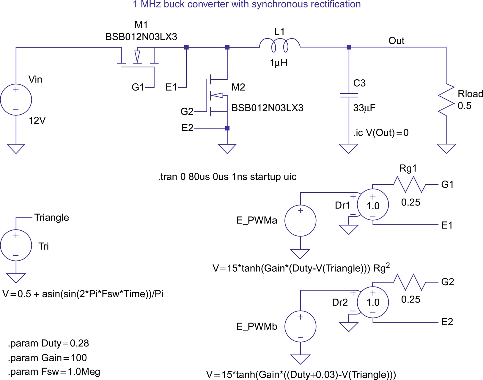
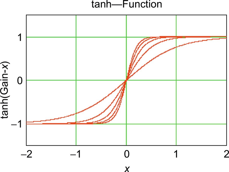
For the generation of the gate-drive signals, the carrier wave is compared with a control signal that can have values between 0.0 and 1.0, corresponding to a duty cycle input between 0% and 100%. Dependent voltage sources E_PWMa and E_PWMb in Fig. 44.1 generate the PWM signals for the MOSFETs M1 and M2, which are included in the LTspice library. A hyperbolic tangent function is used to create a PWM waveform with smooth transitions to aid in convergence. Fig. 44.2 shows a plot of a hyperbolic tangent function to illustrate the concept. The Gain parameter is used to steepen the curve to resemble realistic PWM signal transitions. In Fig. 44.2, the Gain is varied between 1 and 5. In the control functions for E_PWMa and E_PWMb, the factor 15 in front of the tanh function generates an output voltage that varies between −15 and +15 V. Note the inverse polarities on the inputs of sources Dr1 and Dr2 generate the complementary gate-drive signals.
Careful inspection of Fig. 44.1 shows that 3% duty cycle 0.03 is added to generate the gate-drive signal of the lower (synchronous rectification) MOSFET to create some blanking time between the drive signals and avoid cross conduction between the MOSFETs M1 and M2.
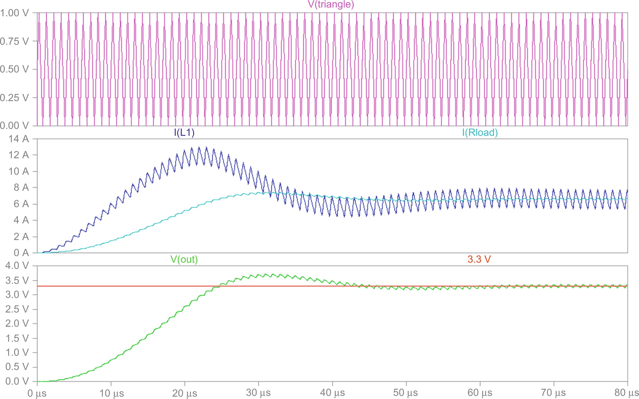
Fig. 44.3 shows the calculated voltage and current traces for the synchronous buck converter. The top-level pane shows the generated triangle carrier. It has a frequency (Fsw; see parameter statement in Fig. 44.1) of 1.0 MHz. The graph below the triangle signal shows the inductor current and the current in the load resistor. The bottom trace shows the capacitor voltage, which has a steady-state value of 3.3 V.
In addition to the cycle-by-cycle simulation of a DC-DC converter, it is also possible to use a time-averaged replacement for the MOSFET transistors used in the circuit in Fig. 44.1. In fact, a common time-averaged model can be used for the buck, the boost, the buck-boost, and the Cuk converter as long as they operate with continuous inductor current. The time-averaged model has the advantage that it can run much faster since it does not have to follow each switching transition. It is also possible to perform DC and AC sweep analyses. A DC sweep would sweep the duty cycle over a wide range and show the output voltage as a function of the duty cycle. An AC sweep analysis would sweep the frequency of an AC signal, which is superimposed on top of the duty cycle bias signal. The AC sweep allows the study of the behavior of the converter, including a feedback control system, in the frequency domain for traditional stability analysis and system tuning. A detailed description of this time-averaged modeling technique, including detailed examples, is given in [6].
To illustrate the capabilities of the LTspice simulation program, the next example shows a complete three-phase inverter using six power MOSFETs. This circuit is shown in Fig. 44.4. Such an inverter needs antiparallel diodes connected across each power semiconductor to ensure that the load current can flow continuously. These diodes are often called freewheeling diodes. Here, the freewheeling diodes are an integral part of every power MOSFETs (body diodes) and are therefore not visible. The inverter drives a three-phase load, which represents the 5 hp induction motor used later. The R and L values represent rated load conditions. The load is connected to the inverter output terminals via labels (A,B,C).
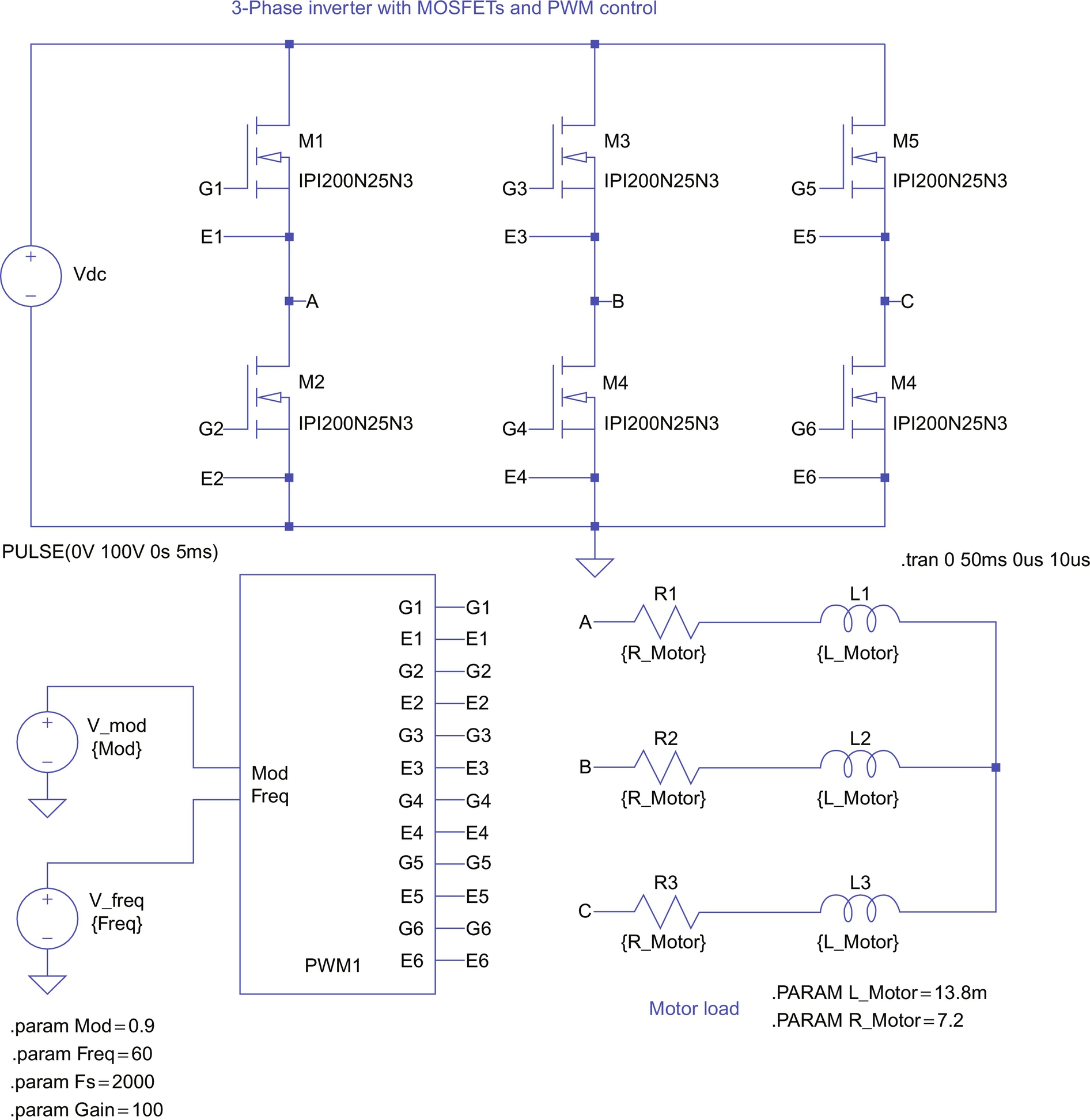
Due to the number of elements involved, the circuit for the gate-drive signal generation is contained in a custom part named PWM1. Custom parts like this can easily be generated using the “Hierarchy—Create a New Symbol” menu path in the LTspice schematic editor. Double-clicking on the part reveals the associated subcircuit that is shown in Fig. 44.5. The arrow-shaped symbols on the right side of Fig. 44.5 named G1, E1, G2, etc. are called interface ports and are the outputs of the gate-drive circuit to the MOSFETs. These interface ports provide the connection between the subcircuit and the ports of the custom part. These ports on the custom part are created using the “Edit—Add Pin/Port” menu path in the LTspice schematic editor. The arrow-shaped symbols on the left side of Fig. 44.5 are inputs for the fundamental output frequency and the modulation index. The names of these ports in the subcircuit (must!) correspond to the names of the ports of the custom symbol.
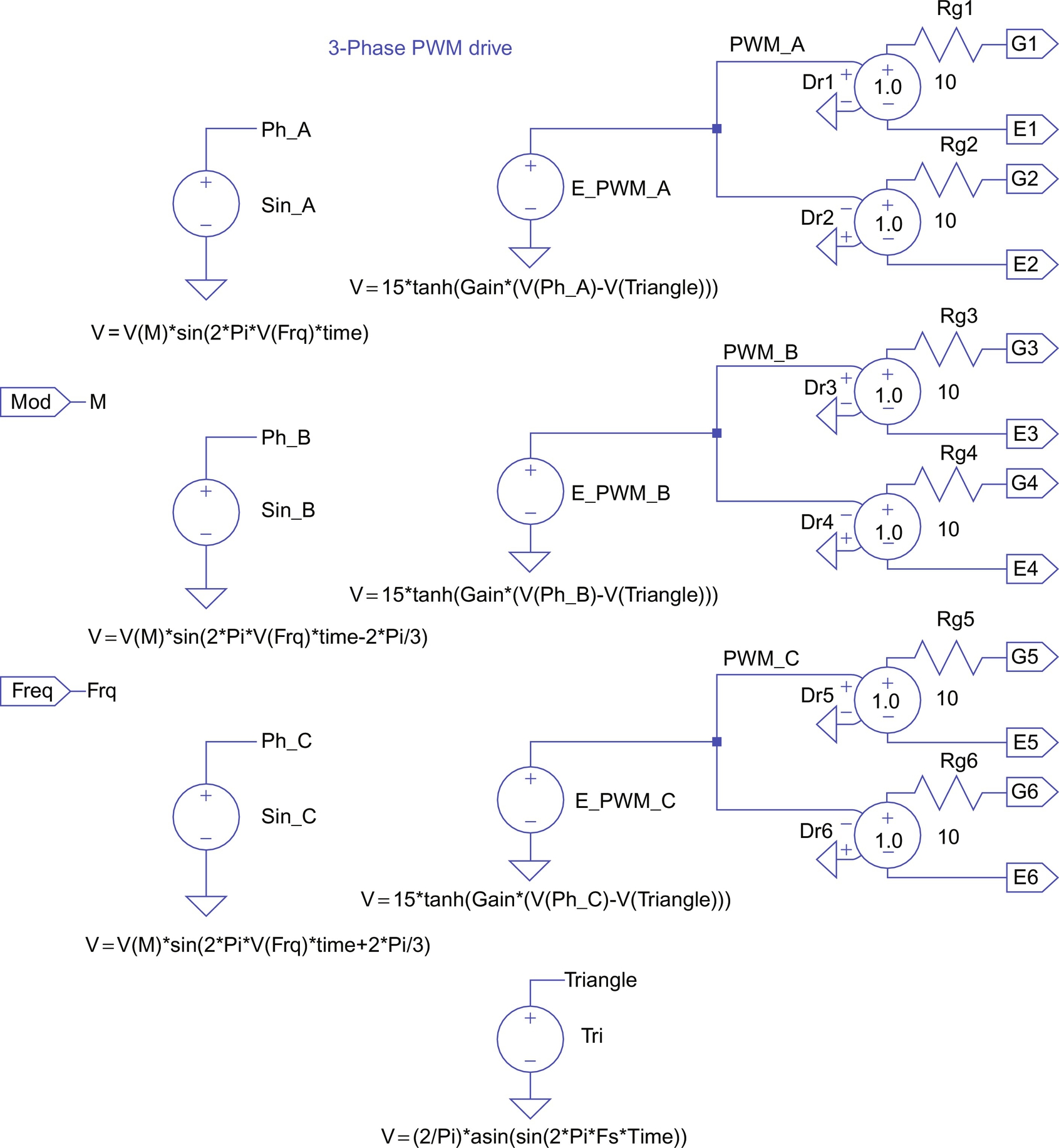
The circuit shown in Fig. 44.5 is similar to the gate-drive generation circuit discussed before. As in the PWM generation circuitry shown in Fig. 44.1, a triangular carrier is compared with a reference signal. In this case, three reference signals, one for each phase, are compared with 3 PWM sources (E_PWM_A, E_PWM_B, and E_PWM_C) to create the gate-drive signals for all three phases. Again, the factor 15 in front of the tanh functions generates an output voltage that varies between −15 and +15 V for driving the gates of the MOSFETs. Here, the triangular carrier signal is symmetrical with respect to the time axis and covers the range from ![]() to 1.0. The closed form expression for the triangular carrier is given by Eq. (44.2):
to 1.0. The closed form expression for the triangular carrier is given by Eq. (44.2):
The three reference signals are sinusoidal signals with equal amplitude and a relative phase shift of 120°. For linear modulation, the amplitude range of the reference signals is limited to the amplitude of the triangular carrier, for example, 1 V. The ratio of the reference wave amplitude and the (fixed) carrier amplitude is called amplitude modulation ratio Mod. In the circuit shown in Fig. 44.4, Mod has a value of 0.9. This value is defined by a parameter symbol at the top level and therefore represents a global parameter, which is visible throughout all levels of the hierarchy. The amplitude of the phase-to-neutral voltage of each inverter leg is equal to half of Vdc (shown in Fig. 44.4) multiplied with the amplitude modulation ratio. The frequency and wave shape of the phase-to-neutral voltage of each phase leg is equal to the reference waveform if the high-frequency components resulting from the carrier wave are filtered away. Each inverter leg can be viewed as a power amplifier for its reference voltage. In fact, in drive applications, inverters are often called “servo-amplifiers.” The load typically reacts only to the low-frequency components of the inverter output voltage. The high-frequency components, which include the triangular carrier frequency (also called switching frequency) and its harmonics, are typically “just a blur” for the load. These are especially true in recent times, where switching frequencies of 20 kHz and above are possible. As an added benefit, audible noise is avoided at these frequency levels.
The complementary sources Dr1/Dr2, Dr3/Dr4, and Dr5/Dr5 in combination with the gate resistors will generate the control voltages for the transistor pairs of each leg. Using this circuitry will ensure that during switching transitions in each phase leg, the gate voltage of the transistor that is turning off will fall below the turn-on threshold before the gate voltage of the transistor that is turning on reaches that threshold. Therefore, a shoot through, meaning a short circuit between the positive and negative bus, is avoided.
Fig. 44.6 shows the simulation results for the three-phase inverter. The timescale is slightly stretched, to better show the details of the PWM signals. The line-to-line voltage VAB and the load current in all three phases are shown. Due to the inductors contained in the load, the current cannot instantaneously change and follow the PWM signal. Therefore, the load currents are almost pure sinusoids with very little ripple. This is representative of the real line currents in induction motors.
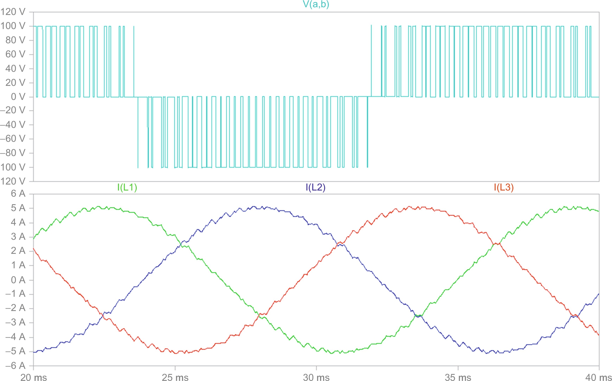
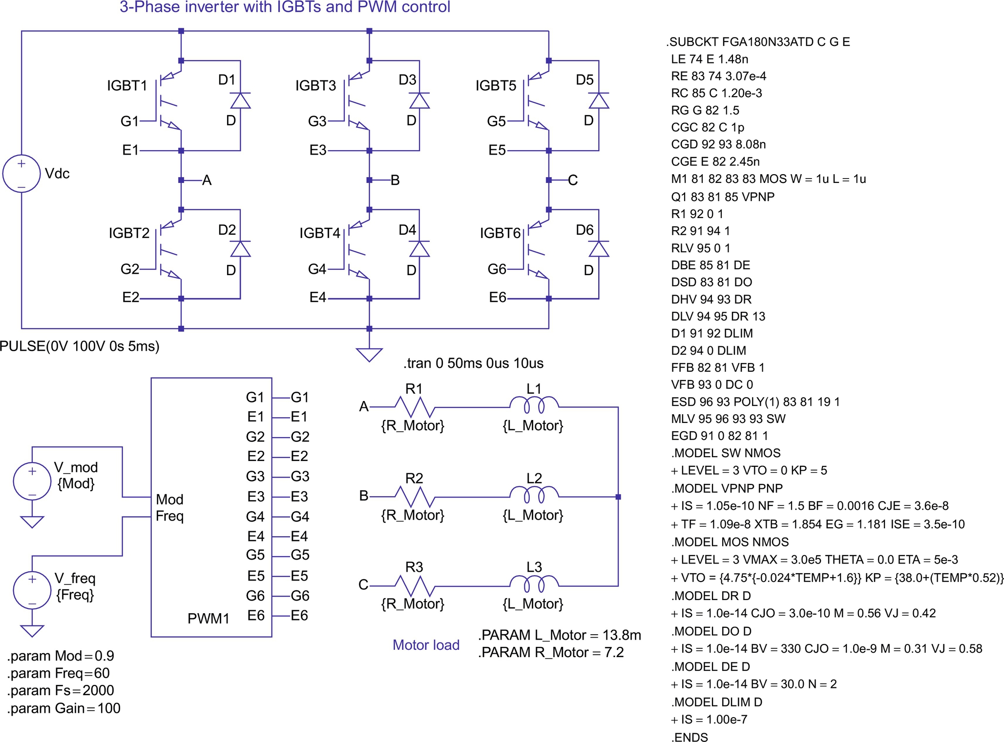
Fig. 44.7 shows an example where the MOSFETs in Fig. 44.4 have been replaced with insulated gate bipolar transistors (IGBTs). The spice model of the particular IGBTs shown here is included on the right side of the schematic. Note that freewheeling diodes are needed, if IGBTs are used. The freewheeling diodes carry the load current when the IGBTs are turned off to provide a continuous path for the current. This is very important, since the load can have a substantial inductive component. Whenever the diodes are conducting, energy flows momentarily back to the source. In the case of power MOSFETs, the diodes (often called body diodes) are an integral part of the device. In the symbol graphic of LTspice, these body diodes are not shown for MOSFETs. For this circuit, the gate-drive circuit and the results are the same as for the three-phase inverter with power MOSFETs. This circuit returns the same results than the one shown in Fig. 44.6 except that the simulation runs a lot longer (minutes rather than seconds) due to the complexity of the IGBT models.
44.4 Simulations of Power Electronic Circuits and Electric Machines
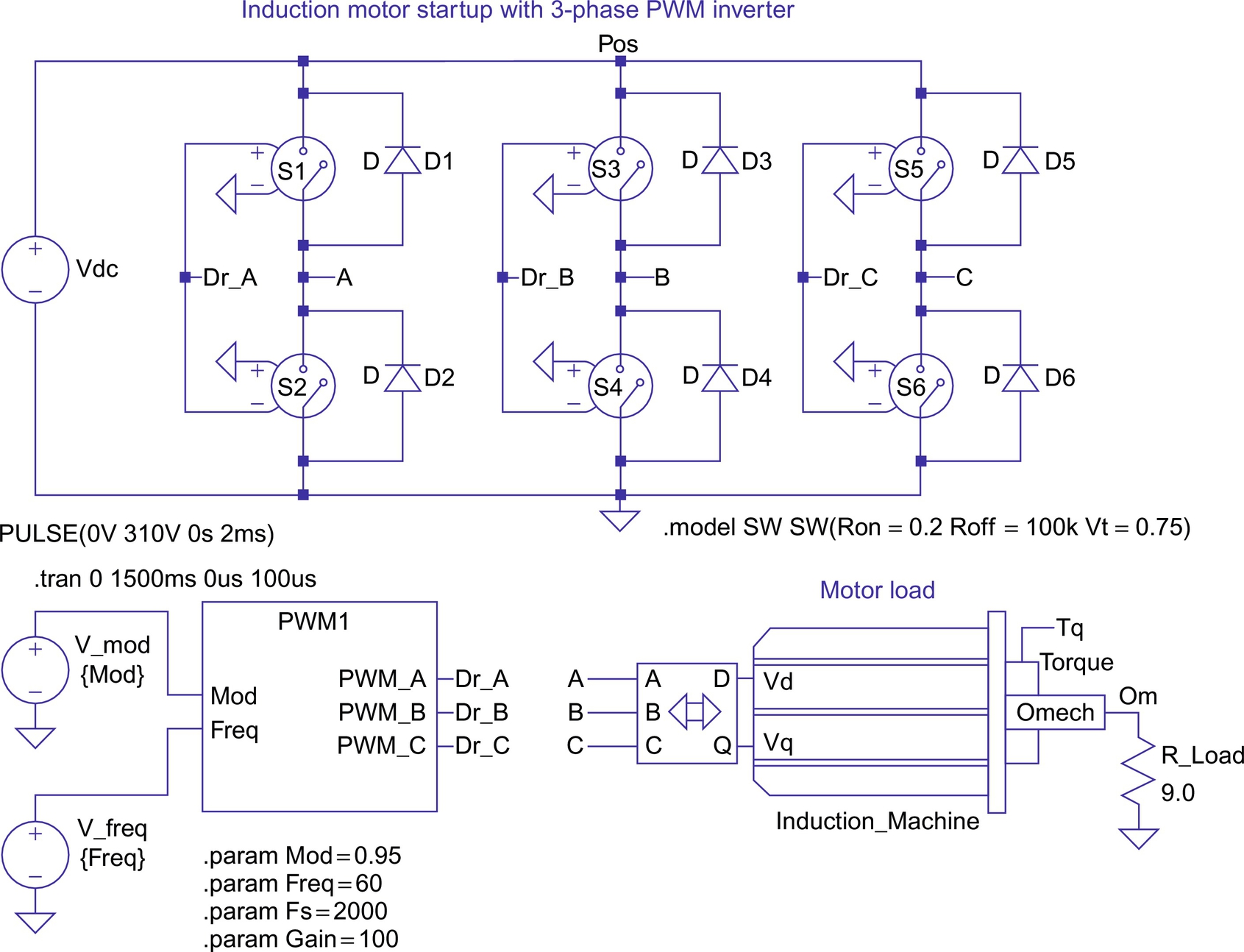
In the following, the start-up of an induction motor, fed by a three-phase inverter similar to the ones shown in Figs. 44.4 and 44.7, is presented. For this purpose, the simple passive load in Figs. 44.4 and 44.7 has been replaced by a complete dynamic model of an induction motor. Also, the MOSFETs or IGBTs from Figs. 44.4 and 44.7, respectively, have been replaced by generic voltage-controlled switches. This will increase the simulation speed even more dramatically compared with the case with IGBTs with very little effect on accuracy since this simulation is meant to study the start-up behavior of an induction motor. For this and further discussions, it is assumed that the reader is familiar with the theory of induction machines and in particular their dynamic behavior. A number of excellent references are given at the end of this chapter [4,5,7,8]. The induction motor symbol represents the electromechanical model of an induction motor. The model is suitable for studies of electric and mechanical transients and steady-state conditions. The output pin on the motor shaft represents the mechanical output. The voltage on this pin represents the mechanical angular velocity using the relation 1 V=1 rad/s. In addition, any current drawn from or fed into this terminal represents applied motor or generator torque according to the relation 1 A=1 N m. Due to these definitions, the electric power associated with the voltage of the motor shaft (with respect to ground) is identical to the mechanical power. Following the well-known theory, the induction motor model has been derived for a two-phase (direct and quadrature, D, Q) equivalent motor. Attached to the motor is a bidirectional two-phase to three-phase converter module. This module is voltage and current invariant. This means that the voltage and current levels in the two-phase and the three-phase machine are equal. Consequently, the power in the two-phase machine is only two-thirds of the power in the three-phase circuit. This is accounted for in the calculation of the electromagnetic torque (factor 3/2; see Eq. (44.4)). The internally generated torque can be monitored on the output labeled Torque on top of the sleeve around the motor shaft. The linear load in Fig. 44.8 is a symbol that represents an appropriately sized resistor to the ground representing rated power that is 5 hp for this example.
In Fig. 44.8, the motor is represented by a custom symbol called induction machine. The symbol can be easily created using the “Hierarchy—Create a New Symbol” menu path in the LTspice schematic editor. The editor provides standard graphic elements (lines, rectangles, circles, etc.) so that professional-looking symbols can easily be created.
Double-clicking on the motor symbol reveals the associated subcircuit that implements its function. This subcircuit is shown in Fig. 44.9. The left part of this subcircuit represents the electric model. The electric model calculates the stator and rotor currents, with the stator voltages and the mechanical speed of the machine being input parameters. However, it is also possible without any changes to feed stator currents (with controlled current sources) into the D and Q inputs. This option is useful for vector control applications, which are discussed later.
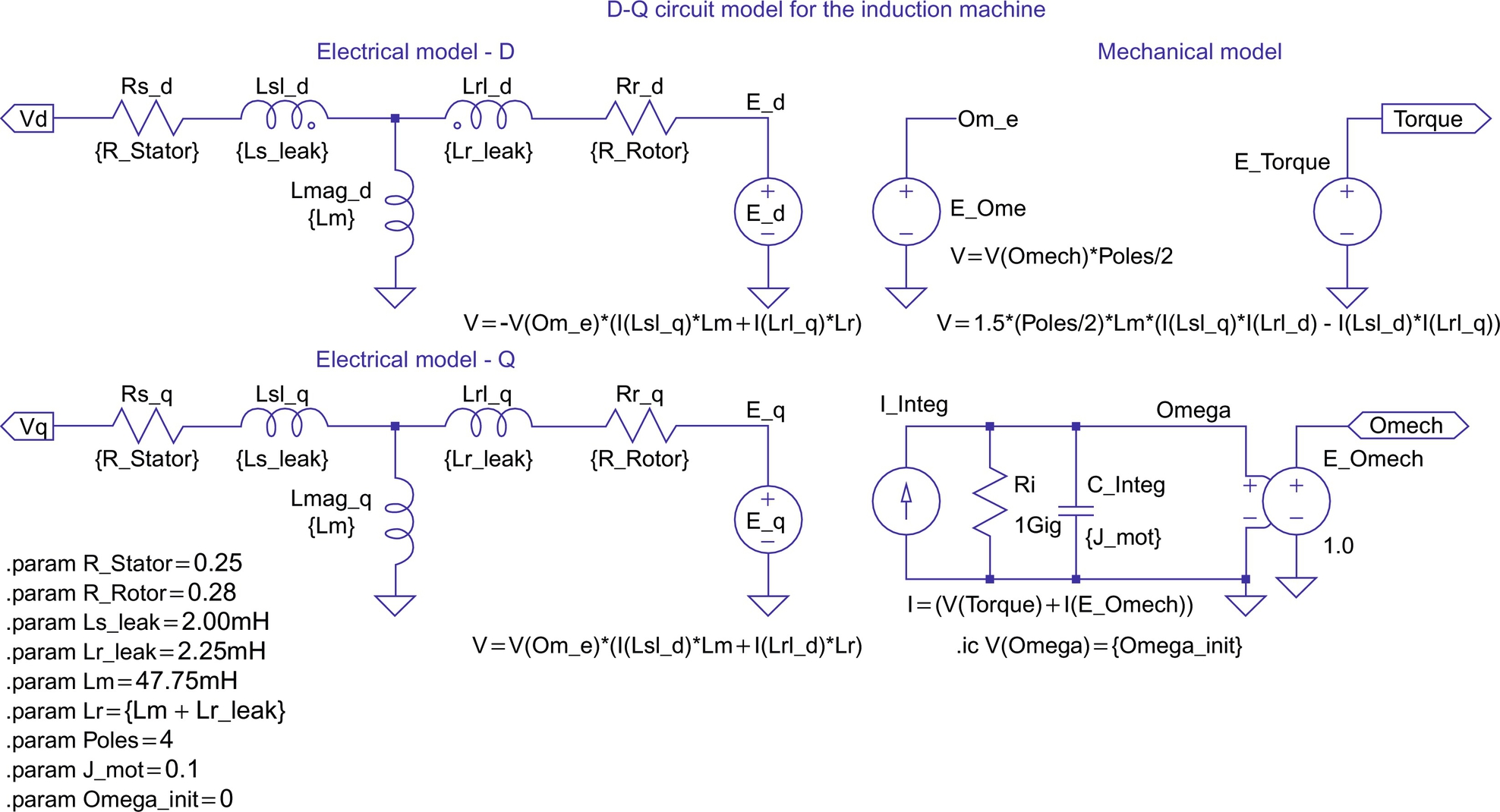
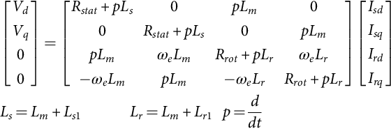
The equation system for the electric model of a two-phase induction machine is given by Eq. (44.3). The theory for this equation system is derived in [4,5,7,8]. The equation system and the model are formulated for the stationary reference frame. This reference frame assumes that the frame of the machine is stationary and the voltages and currents of the rotor are equivalent AC values with stator frequency.
From machine theory, we know that the actual rotor currents have slip frequency. Another reference frame is the synchronous (also called excitation) reference frame. In this reference frame, the stator of a fictitious machine is assumed to rotate with synchronous speed. The advantage of this reference frame is that the input frequency is zero (DC), which makes it easy to derive the principle of vector control by extending the theory of DC machines to AC machines:
In typical implementations of vector control using digital signal processors (DSPs), the synchronous reference frame is used internally to calculate the reference values for the currents in the D- and Q-axis. These values are then transformed to the stationary reference frame in an additional step. Sometimes, still other reference frames are used, and it is possible to generate a universal electric model with a reference frame speed input. This model could then be used for any reference frame.
The electric model in Fig. 44.9 implements the equation system shown in Eq. (44.3). The circuit closely resembles the well-known T-equivalent circuit for the steady-state analysis of induction machines. Two instances of the T-equivalent circuit are necessary to implement the two-phase (D, Q) model. The right part of the schematic in Fig. 44.9 represents the mechanical model. This circuitry calculates the internally generated electromagnetic torque, using the rotor and stator currents as input values. The equation for the internal electromagnetic torque of the induction machine is given by Eq. (44.4) [4,5,7,8]. The factor 3/2 accounts for the fact that the real motor is a three-phase machine. The generated torque is used to calculate the angular acceleration of the motor shaft considering the load torque and the moment of inertia. Integration of the angular acceleration yields the rotor speed, which is used in the electric model:
Since almost all induction machines are three-phase machines, it is often desirable to have a machine model with a three-phase input. Therefore, a bidirectional two-phase to three-phase converter module, which can be attached to the motor, has been developed. A subcircuit for this module is shown in Fig. 44.10.
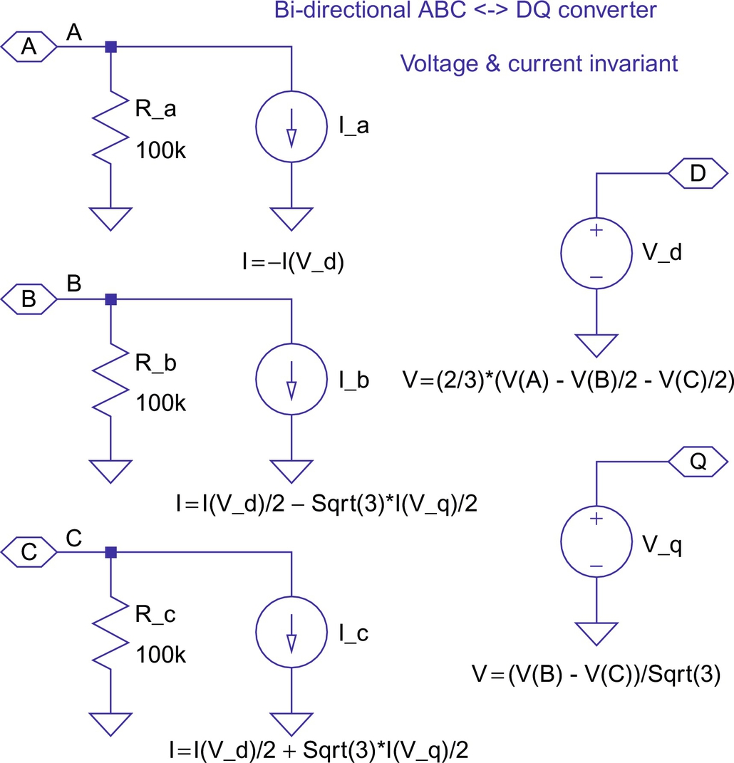
This circuit is truly bidirectional, meaning that the circuit can be fed with voltage or current sources from either side. The equation system for this voltage and current-invariant transformation is given by Eq. (44.5). This transformation is sometimes called “Clark” or “ABC-DQ” transformation. The voltage V0 in Eq. (44.5) denotes a zero-sequence voltage, which is assumed to be zero and not implemented in the subcircuit shown in Fig. 44.10. This voltage would only have nonzero values for unbalanced conditions. An interesting detail of the subcircuit in Fig. 44.10 is the addition of high-value resistors on each input. These resistors provide a small current path from the three-phase input to the ground and ensure stable operation if the module is fed with current sources;
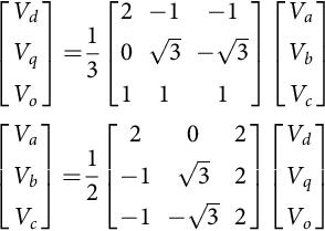
Fig. 44.11 shows the result for the start-up of the induction motor for the circuit of Fig. 44.8. The motor is a 5 hp, 208 V, 4-pole machine. The detailed parameters are shown in Table 44.1. The PWM generation was derived from the example shown in Fig. 44.4. The top trace in Fig. 44.11 shows the mechanical angular velocity with a scale of 1 V=1 rad/s. The middle trace shows the developed electromagnetic torque, including the level for the rated steady-state torque (20 N m as commanded by the load in Fig. 44.8) and the zero level. This graph shows the typical oscillatory torque production of the induction machine for an uncontrolled line start. The scale for this graph is 1 V=1 N m. The bottom trace of Fig. 44.11 shows the input current for phase A.
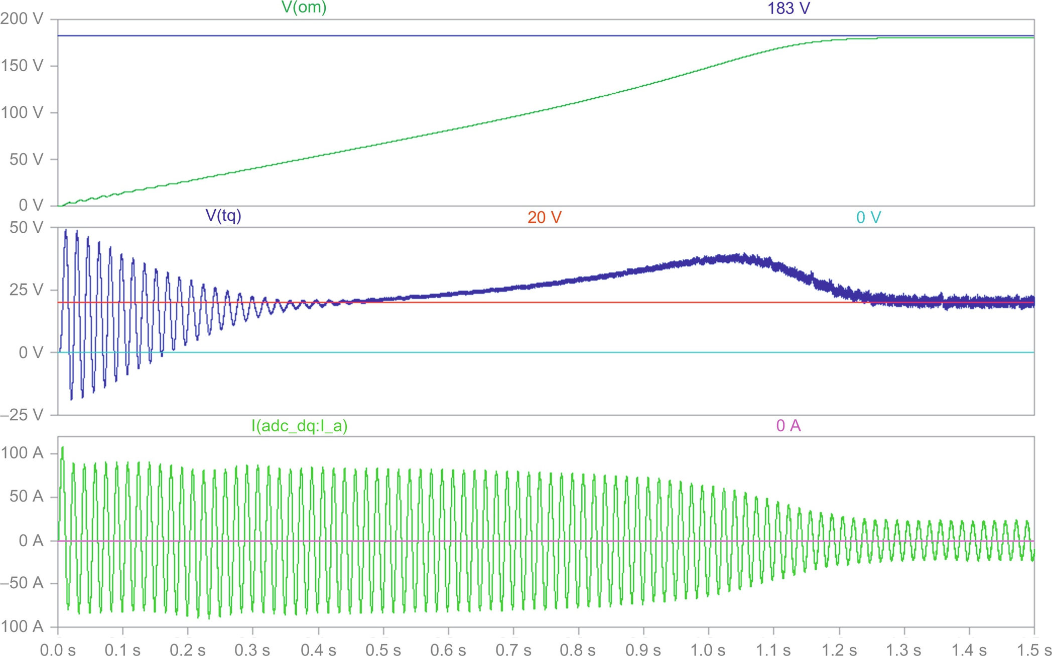
Table 44.1
List of all attributes used for the 5 hp, 208 V, 4-pole induction motor
Attributes
R_Stator=0.25 Ω
R_Rotor=0.28 Ω
Ls_leak=2.00 mH
Lr_leak=2.25 mH
Lm=47.75 mH
Ls=Lm+Ls_leak
Lr=Lm+Lr_leak
kT=1.5⁎(Poles/2)⁎Lm/Lr
Tau_r=Lr/R_Rotor
Sigma=1−Lm⁎Lm/(Ls⁎Lr)
Poles=4
J_mot=0.1 kg m2
Omega_init=0
It is evident that the current trace is an almost perfect sinusoid, despite the fact that the input voltage is a PWM waveform. Also, the trace for the torque shows only a small high-frequency ripple. The reason is, of course, that the motor windings are inductive and represent a low-pass filter for the applied voltages. Nevertheless, recent research suggests that filtering the output voltage of the inverter is advantageous anyway, because it significantly reduces the voltage stress on the windings and suppresses displacement currents through the bearings [9].
44.5 Simulations of AC Induction Machines Using Field Oriented (Vector) Control
The following examples will demonstrate the use of LTspice for simulations of field-oriented control (FOC) of AC induction machines. Again, it is assumed that the reader is familiar with the basics of induction machine theory. Often times, FOC is also called vector control, and both expressions can be used interchangeably. The theory of vector control is described in detail in [4,7,8]. The idea was originally proposed in the 1960s by Hasse and Blaschke, working at the Technical University of Darmstadt [10]. The author had the privilege of taking one of Prof. Hasse's classes on machine control as an undergraduate student. The basic idea of FOC is to inject currents into the stator of an induction machine such that the magnetic flux level and the production of electromagnetic torque can be independently controlled and the dynamics of the machine resembles that of a separately excited DC machine. The previously discussed two-phase model for the induction machine is very helpful for studies of vector control and shall be used in all examples. If a two-phase induction motor model for the synchronous (or excitation) reference frame is used, the similarities between the control of a separately excited DC machine and vector control of an AC induction machine will be most evident. In this case, the D input corresponds to the field excitation input of the DC machine, and both inputs are fed with DC current. Assuming unsaturated machines, the current into the D input of the induction machine or the field current in the DC machine directly controls the flux level. The Q input of the induction machine would correspond to the armature winding input of the DC machine, and again, both inputs would receive DC current. These currents would directly control the production of electromagnetic torque with a linear relation (constant kT) between the current level and the torque level. Furthermore, the Q component of the current would not change the flux level established by the D component (no cross coupling). To make such a simulation work, it would finally be necessary to calculate the slip value that corresponds to the commanded torque and use this value to calculate the speed of the synchronous reference frame of the machine model.
Of course, this is very interesting from an academic standpoint, and the author uses this example in a semester-long lecture on machines and drives. However, it should again be noted that a machine represented by a model with a synchronous reference frame would have a stator, which rotates with synchronous speed. Of course, this is not realistic, and therefore, it is more interesting to generate a simulation example that uses the previously discussed motor model for the stationary reference frame. This motor must be supplied with AC voltages and currents with a frequency determined mostly by the rotor speed and to a small extent (slip value) by the commanded torque. We still compute DC values representing the commanded flux and torque, but we transform these DC values to appropriate AC values. In the following example, we will assume that we can measure the actual rotor speed with a sensor. For this purpose, many types of sensors are available on the market. If we add the slip speed to the measured rotor speed, we obtain the synchronous speed for the given operating point. We determine the slip speed from the torque command. With this synchronous speed, we can transform the DC flux and torque command values from the synchronous reference frame to the stationary reference frame. We accomplish this by using a rotational transformation according to the matrix equations in Eq. (44.6). This rotational transformation is also called “Park” transformation. As shown in Eq. (44.6), the transformation is bidirectional, and the product of the transformation matrices yields the unity matrix:
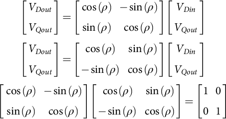
For the following discussion, we shall define the transformation that produces AC values from DC inputs as a positive vector transformation and the reverse operation consequently a negative vector transformation. The matrix equation for the positive vector transformation is shown on the left side of Eq. (44.6). The negative transformation is very useful to extract DC values from AC voltages and currents for diagnostic and feedback control purposes. Both rotational transformations use the angle, α, in the equations. This angle can be interpreted as the momentary rotational displacement angle between two Cartesian coordinate systems, one containing the input values and the other the output values. This angle is obtained by integration of the angular velocity with which the coordinate systems are rotating (typically the synchronous speed).
In summary, we replaced a theoretical motor model using a synchronous reference frame by a reference frame transformation of the supply voltages and currents. In fact, modern DSPs are capable to perform both the Clark and the Park transformations in both directions at very high speeds. These DSPs are well supported with proved reference designs, including free software examples.
Fig. 44.12 shows the top level of a simulation example that implements vector control for an induction machine with a stationary reference frame model. The motor model and the associated subcircuits (Fig. 44.9) are identical to the ones used for the circuit shown in Fig. 44.8. As discussed above, the actual speed of the rotor is used as an input signal for the control unit. This scheme is known as indirect vector control and represents one of the most often used control methods. The symbol for the controller uses the same parameters as the motor. This is necessary to achieve correct field orientation. In real systems, the controller must be told or somehow determine the machine parameters. The machine parameters are contained in .param statements. If these .param statements are used at the top level of the hierarchy, they are global to the simulation, but if they are contained in a subcircuit, they are local to that subcircuit. Here, the vector controller and the induction motor both have local parameters, which enables us to study the influence of parameter mismatch on the performance of the control.
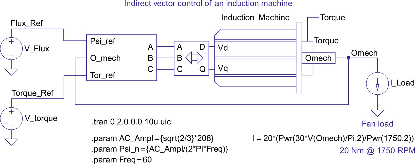
Fig. 44.12 shows a dependent current source that represents a fan load for the motor. The current of this source represents the load torque and is proportional to the square of the mechanical speed of the motor shaft. That speed is represented by the voltage on the Omech terminal. The controlling equation is scaled such that the load draws the rated torque (20 A=20 N m) at rated speed (1750 RPM). In this fashion, many more mechanical properties and devices can be modeled. For example, a mechanical flywheel is simply represented by a capacitor to the ground. Due to the scaling factors for the angular velocity and the torque, a flywheel with ![]() would be a capacitor with a value of C=1 F. The compliance of a driveshaft (elastic twisting by the applied torque) can be modeled by a series inductor. By including both capacitors and inductors, effects like mechanical resonance can be included in a model.
would be a capacitor with a value of C=1 F. The compliance of a driveshaft (elastic twisting by the applied torque) can be modeled by a series inductor. By including both capacitors and inductors, effects like mechanical resonance can be included in a model.
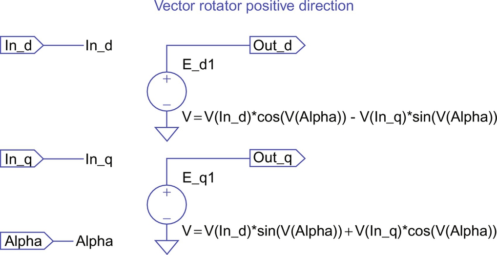
Fig. 44.13 shows the subcircuit for the vector control unit. The central part is a vector rotator for positive direction. This element transforms the DC reference values for the flux (D-axis) and the torque (Q-axis) to the stationary reference frame. The input angle for the vector rotator is the integral of the synchronous angular velocity. The signal called Omech is the measured rotor speed. The subcircuit for the vector rotator is shown in Fig. 44.14.
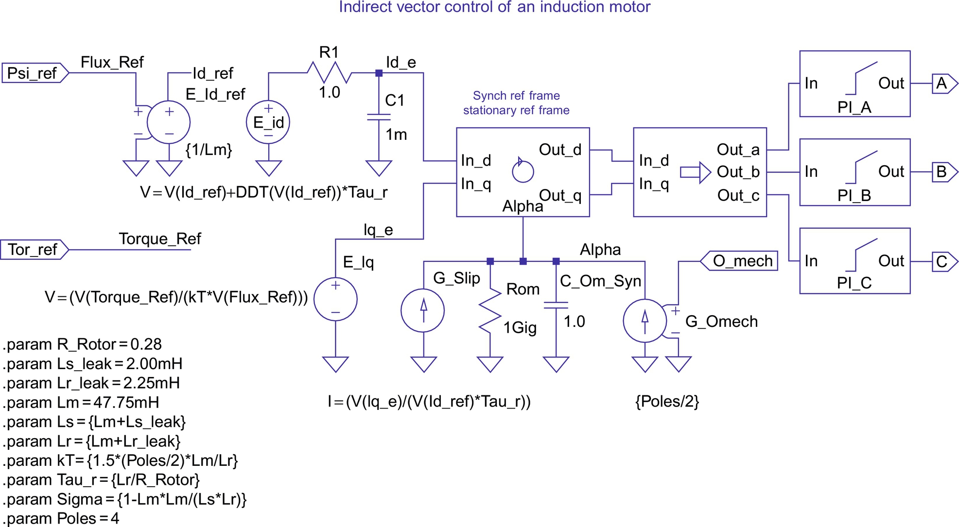
This speed is multiplied with the number of pole pairs (poles/2) to obtain the electric angular velocity. Then, the slip value (see Eq. (44.7) for slip frequency calculation for vector control) appropriate to the torque command is added, and the resulting signal is routed through an integrator to generate the input angle for the vector rotator.
In the D-axis, a differentiator function DDT(V(Id_ref)) is used in a compensation element (see Eq. (44.8) for D-axis reference current for vector control) that assures that the actual flux in the machine follows the commanded signal without delay. The input and output values of the vector rotator are voltage signals that correspond 1:1 to current signals. (In a real controller, the currents are typically scaled values in the memory of a DSP.) The vector controller calculates the appropriate currents that need to be injected into the machine to perform as desired. The currents are then transformed into three-phase values using the equations of (44.5) and fed into three voltage sources with PI current loop feedback that represents a realistic implementation using a voltage-source PWM inverter. Alternatively, the PI current loops could be replaced with ideal current sources that are available in LTspice:
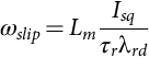
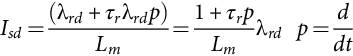
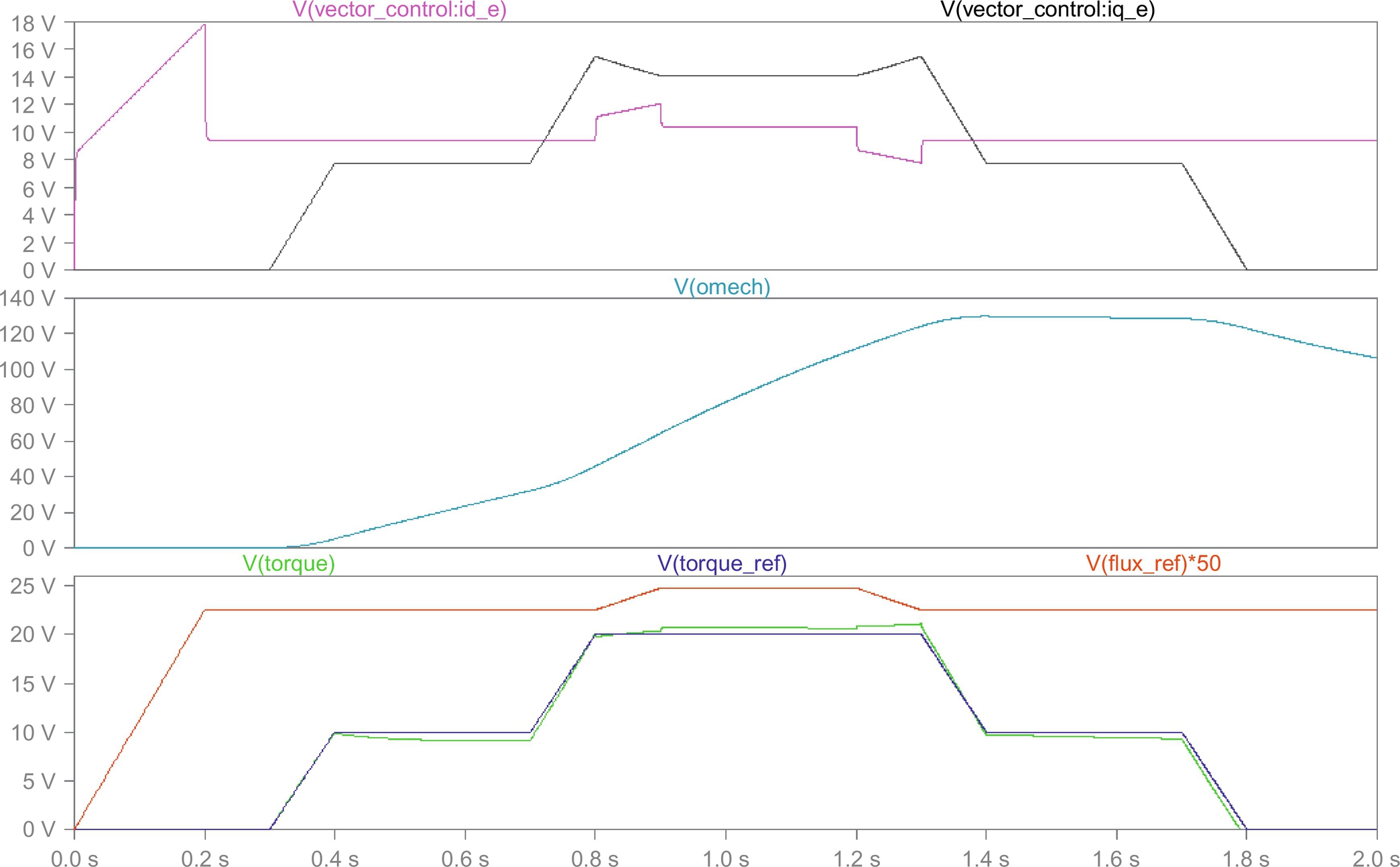
Fig. 44.15 shows the results obtained for the circuit shown in Fig. 44.12 with perfect tuning of the vector controller. Perfect tuning means that the controller precisely knows all motor parameters at all times (including resistance changes due to heating of the windings). The two traces in the pane at the top of Fig. 44.15 represent the traces for the D and Q input signals of the vector rotator. The upper trace in the bottom pane of Fig. 44.15 shows the reference value for the flux scaled by a factor of 50. It is evident that the flux level is being changed at the same time when 20 N m of torque is commanded (and produced). This proves that with exact tuning the torque and the flux can be independently controlled, which is true for correct FOC. Below the trace for the flux reference are the traces for the torque reference and the actual torque, which are perfectly on top of each other. This provides the easiest way to judge the quality of the correct field orientation.
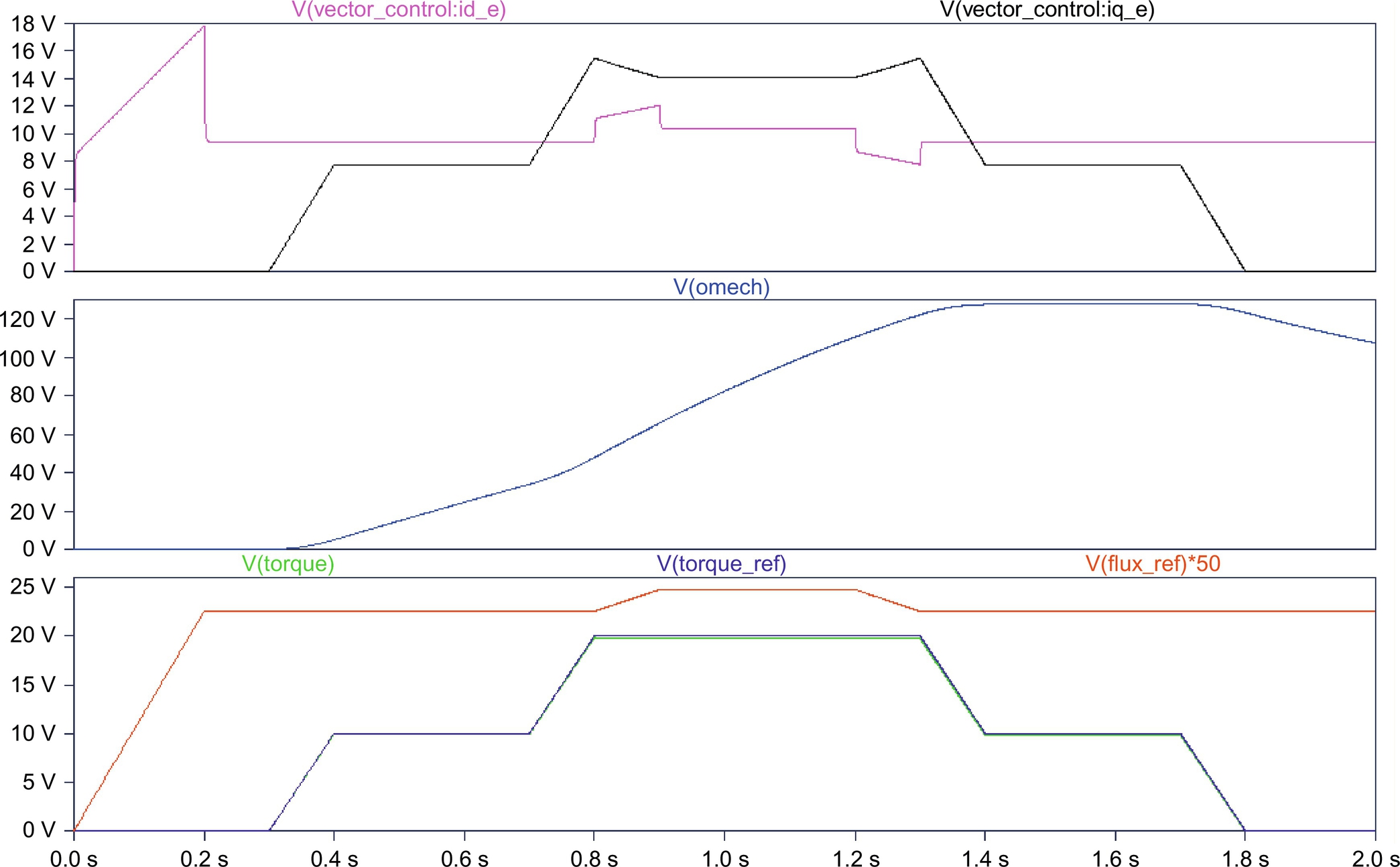
The center pane shows the trace for the mechanical angular velocity. It can be seen that the machine accelerates whenever torque is developed and slows down due to the load when the torque command is driven to zero.
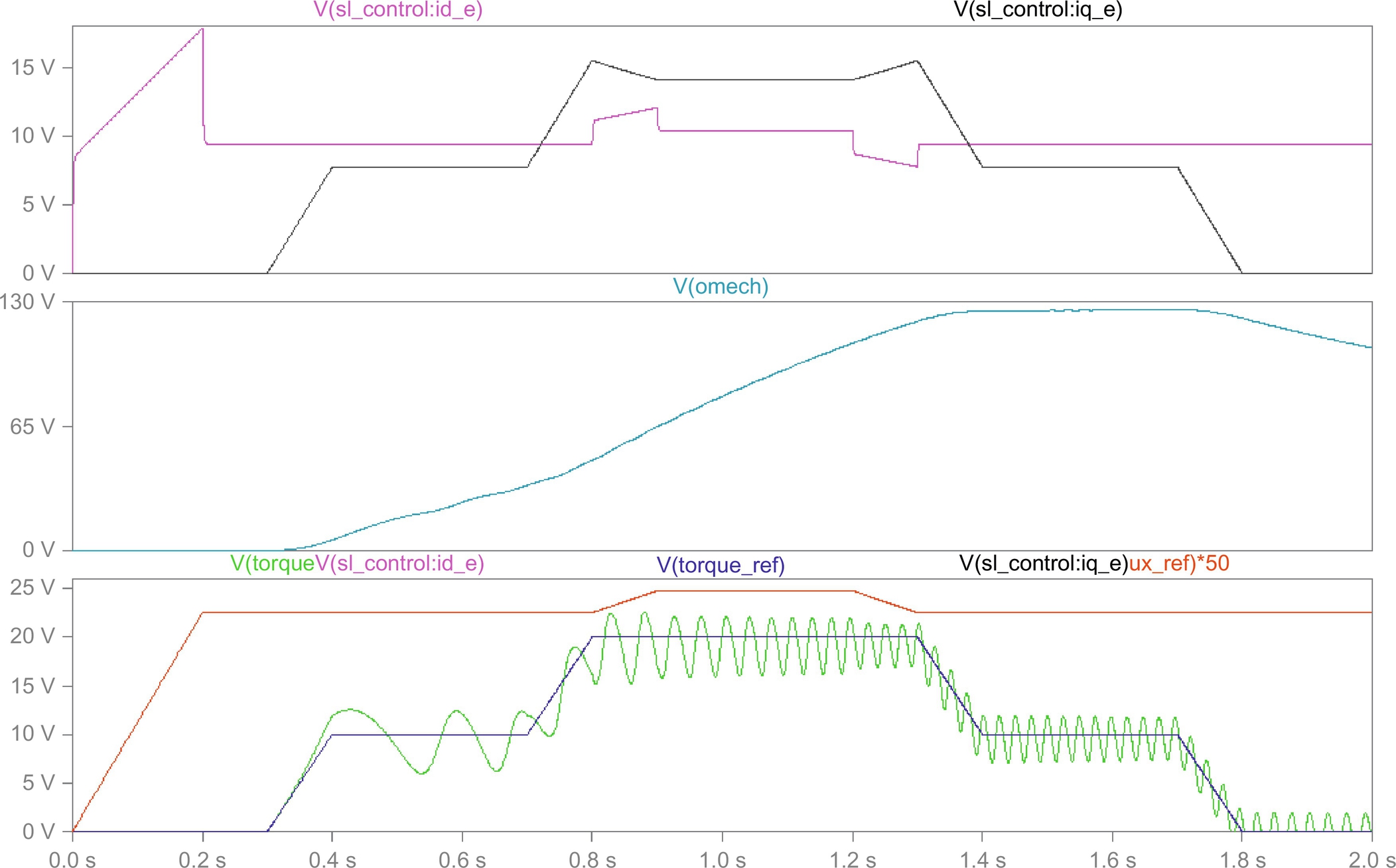
Fig. 44.16 is an example of the results obtained from a detuned vector controller. The circuit is identical to the circuit in Fig. 44.12, except for the fact that the rotor resistance value in the controller was increased to 125%, which is thought to be attributed to heating of the rotor bars. It is obvious that the traces for the commanded and the actually produced torque are no longer identical. This is especially true, during times when the flux is changing. Detuning is actually a real problem in industrial vector control applications. Detuning is caused by the fact that the machine parameters are not precisely known to begin with and/or are changing during the operation of the machine. The values of the winding resistance are most commonly increasing due to heating of the machine during operation at high load.
44.6 Simulation of Sensorless Vector Control Using LTspice
In the previous example, the advantages of vector control have been shown. However, for the implementation of the control scheme, a sensor for the mechanical speed was used. This poses a problem for applications where a vector drive is to be retrofitted into existing equipment. The motor installation may not easily allow the installation of a mechanical speed sensor. Therefore, engineers have thought to replace the mechanical speed sensor with a speed observer, which is a mathematical model that is evaluated by the control processor (typically a DSP), which is also performing the standard vector control computations. The algorithm for the observer uses the measured stator voltages and currents for the D- and Q-axes as input parameters. It also relies on the knowledge of the machine model and on the correct machine parameters (rotor and stator resistance, mutual and leakage inductance, etc.). The following example shows a vector control implementation using a speed observer. The vector controller has been derived from the previous example shown in Fig. 44.13. However, the speed sensor signal was replaced by a speed observer. Careful examination of the derivation [4] of the speed observer reveals that it is easier to calculate the synchronous angular velocity, which is ultimately desired, than the angular velocity of the rotor. Therefore, the observer was modified, and the calculation of the rotor speed and the subsequent addition of the slip speed were foregone. The speed observer used here basically solves the D, Q equation system of the induction machine shown in Eq. (44.3), with the only difference that some of the dependent variables are now independent and vice versa. In addition to the synchronous angular velocity, the observer provides the values of the rotor flux, which could be used in the D-axis signal path.
Fig. 44.17 shows the top level of a simulation project for sensorless vector control. The top view of this circuit is very similar to the circuit for the indirect vector control represented by Fig. 44.12 except for the missing motor-speed feedback. The model for the motor and the motor's parameters are precisely the same as in the example for the indirect vector control. Double-clicking the control block reveals the associated subcircuit, which is shown in Fig. 44.18. As mentioned before, this subcircuit is similar to the subcircuit for the indirect vector control. However, the signal from the motor-speed sensor is replaced by the speed observer. In our case, the speed observer directly provides the synchronous angular velocity. Therefore, it is not necessary to calculate the slip speed and add it to the rotor speed to obtain the synchronous speed.
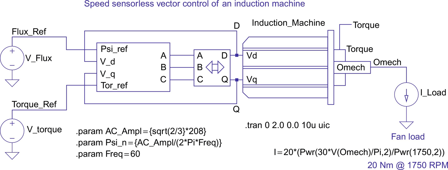
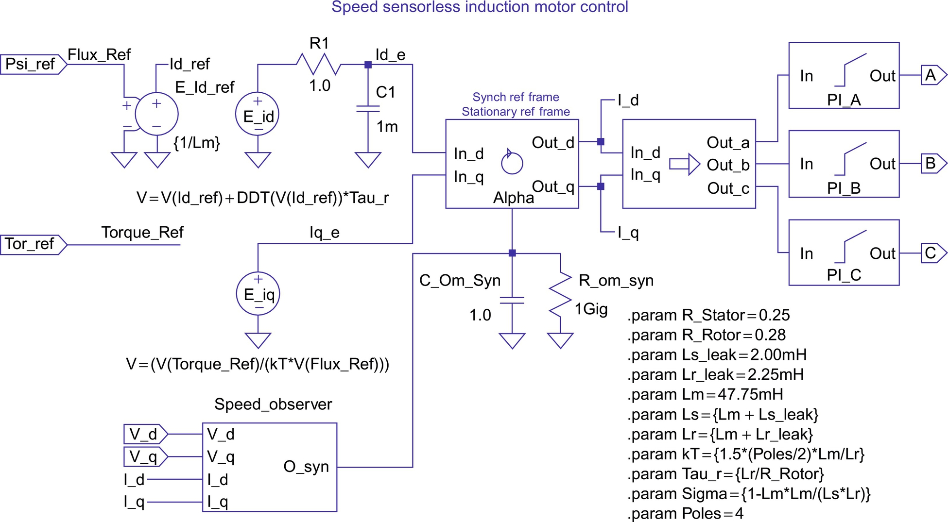
Fig. 44.19 shows the subcircuit for the speed observer. The speed observer uses the stator voltages and currents for the D- and Q-axis as input variables. After subtracting the voltage drop across the winding resistance and the leakage inductance of the stator from the stator input voltage and scaling the result by Lr/Lm, the observer calculates the D and Q components of the rotor flux by integration. Since the input values are in the stationary reference frame, so are the results. The observer also calculates the magnitude of the rotor flux (Eq. (44.9)) and then calculates the synchronous angular velocity (Eq. 44.10) by evaluating the rate of change of the ratio of the D and Q components. The mathematical relationships are given by Eqs. (44.9) and (44.10) [4]:
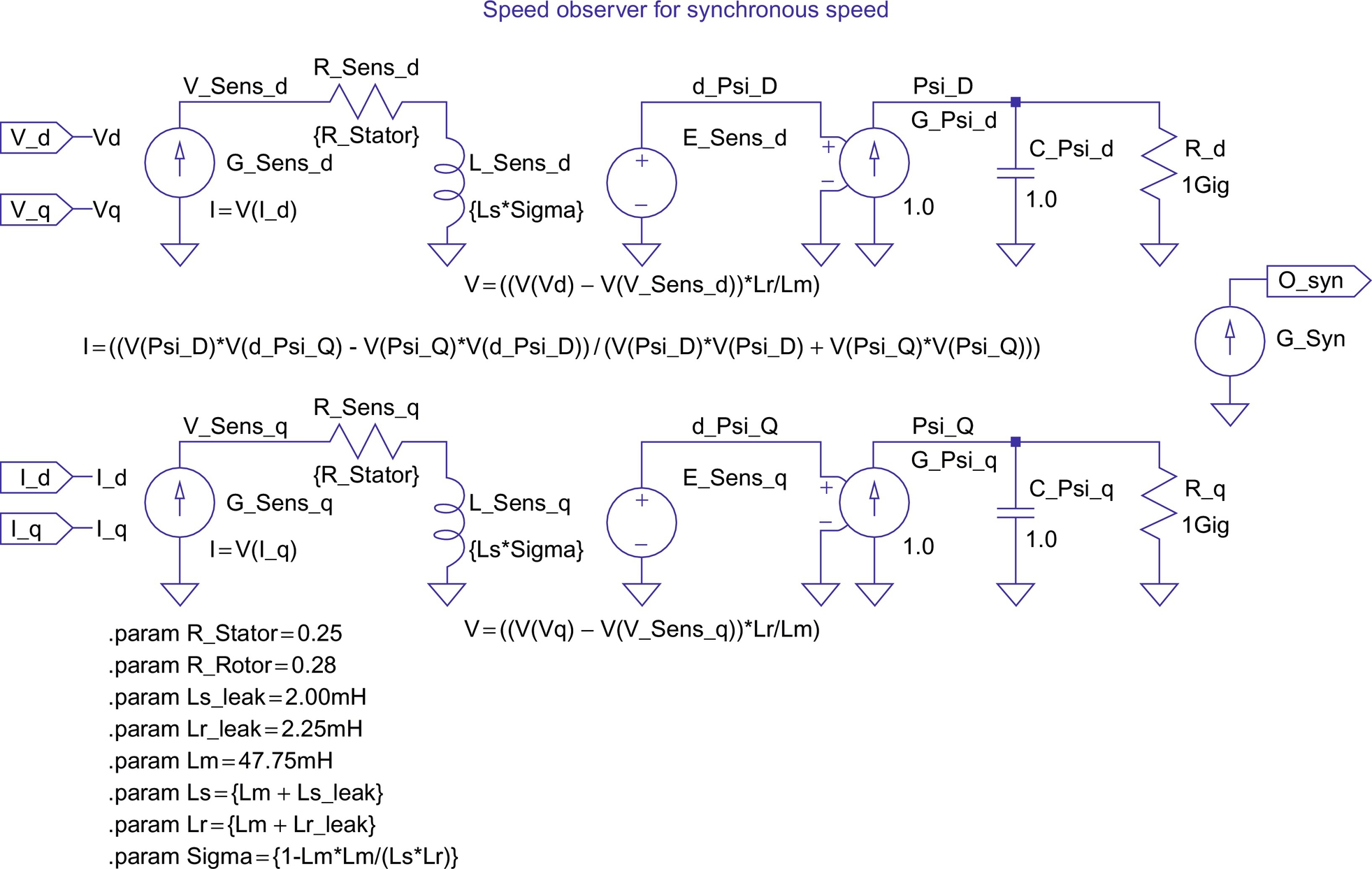
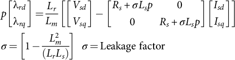
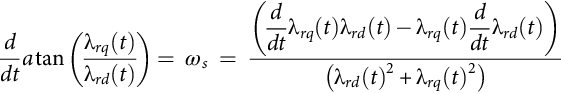
Fig. 44.20 shows the output for the speed sensorless vector control project as it presents itself in the LTspice waveform display for perfect tuning of the speed observer. A comparison of the traces for the torque and the torque command (they are perfectly on top of each other) shows that the scheme works extremely well. It even works for a start from zero speed, which is typically not the case in real systems. The reason is that the uncertainties of the winding resistance values (note that they change with temperature) create errors in observers like this one. The problem is worst at low speeds, because at low speeds and associated low stator frequencies, the uncertain winding resistance represents the largest part of the total machine impedance.
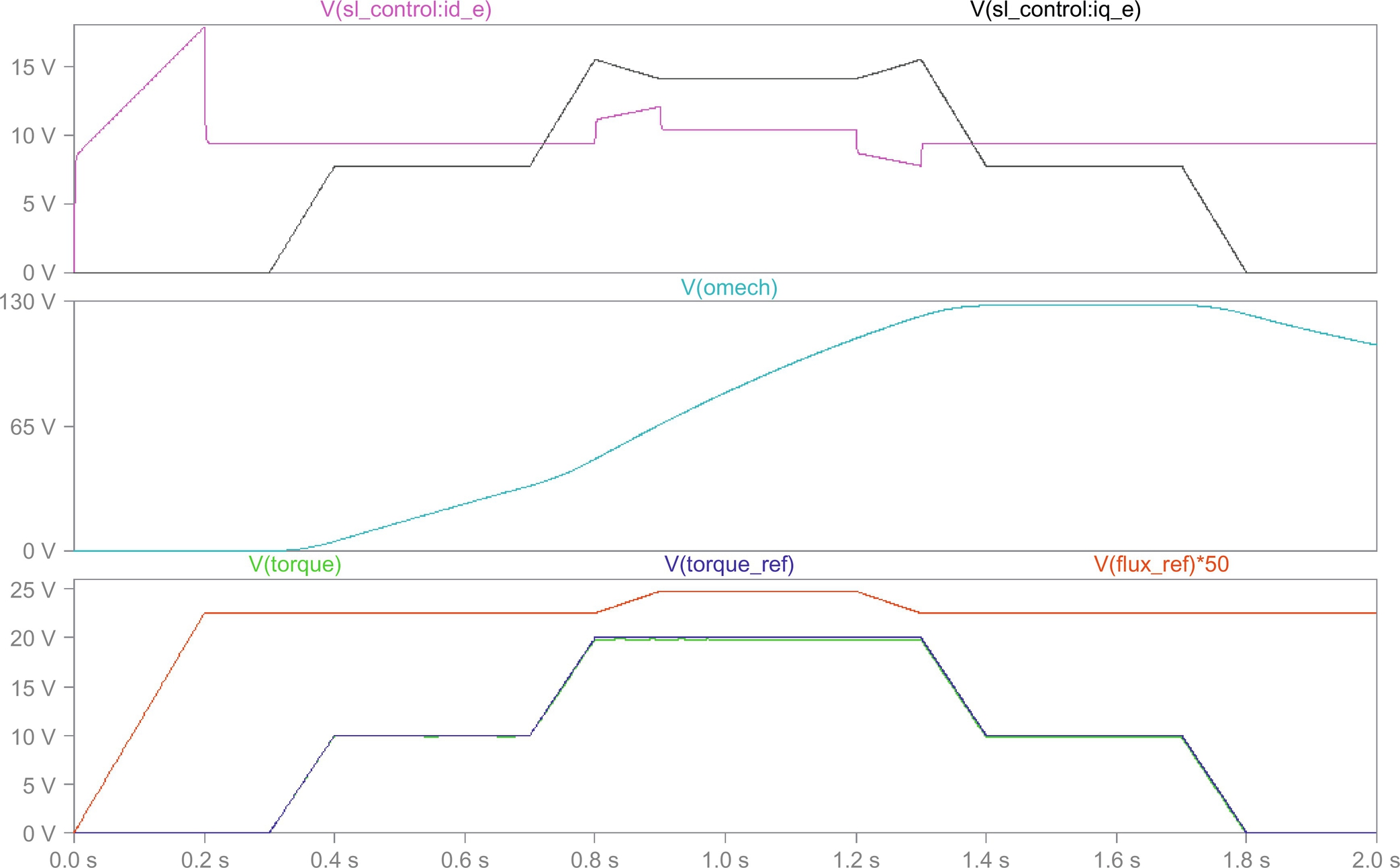
Fig. 44.21 shows the output for the speed sensorless vector control example with increased values for the stator resistance (0.28 Ω instead of 0.25 Ω). A comparison of the traces for the torque and the torque command now shows that the control does not work well in this case. This confirms that at low speeds including zero speed, an actual speed sensor is required for proper field-oriented control.
44.7 Conclusions
In this chapter, the capabilities of LTspice [1] have been used to simulate a number of examples from the power electronics, machines, and drive area. The advantage of LTspice is that it is based on the almost universal spice simulation language, which can be seen as the worldwide de facto standard for circuit simulation. The reader should always validate any model before it is used for critical engineering decisions. It was pointed out in the introduction that model validation often means verification that the limitations of the model are not exceeded.
In addition to the detailed examples, some general guidelines on the uses of simulation for analysis and design have been developed. All tested simulations yielded excellent results. The simulation time for each project shown was typically less than a minute on a contemporary (2016) PC. The author hopes that the reader has gotten an insight and appreciation of the power of modern circuit simulation codes and some useful ideas and inspirations for projects of his/her own.