
Artificial Neural Network Applications in Power Electronics and Electric Drives
Baburaj Karanayil The University of New South Wales, Sydney, NSW, Australia
Muhammed F. Rahman The University of New South Wales, Sydney, NSW, Australia
Abstract
In classical control systems, knowledge of the controlled system (plant) is required in the form of a set of algebraic and differential equations, which analytically relate inputs and outputs. However, these models can become complex, rely on many assumptions, may contain parameters that are difficult to measure, or may change significantly during operation as in the case of the rotor-flux-oriented control induction motor drive. Classical control theory suffers from some limitations due to the assumptions made for the control system such as linearity, time invariance, etc. These problems can be overcome by using artificial intelligence-based control techniques, and these techniques can be used, even when the analytic models are not known. Such control systems can also be less sensitive to parameter variation than classical control systems. This chapter describes the potential of artificial neural networks to track variation parameters in parameters that are used in the rotor-flux-oriented controller of an induction motor drive.
Keywords:
Artificial neural networks; Rotor-flux-oriented controller; Fuzzy-logic systems; Neural function approximator; Induction motor drives; Speed estimator
37.1 Introduction
In classical control systems, knowledge of the controlled system (plant) is required in the form of a set of algebraic and differential equations, which analytically relate inputs and outputs. However, these models can become complex, rely on many assumptions, may contain parameters that are difficult to measure, or may change significantly during operation as in the case of the rotor-flux-oriented control (RFOC) induction motor drive. Classical control theory suffers from some limitations due to the assumptions made for the control system such as linearity and time invariance. These problems can be overcome by using artificial intelligence-based control techniques, and these techniques can be used, even when the analytic models are not known. Such control systems can also be less sensitive to parameter variation than classical control systems.
The main advantages of using artificial intelligence-based controllers and estimators are the following:
• Their design does not require a mathematical model of the plant.
• They can lead to improved performance, when properly tuned.
• They can be designed exclusively on the basis of linguistic information available from experts or by using clustering or other techniques.
• They may require less tuning effort than conventional controllers.
• They may be designed on the basis of data from a real system or a plant in the absence of necessary expert knowledge.
• They can be designed using a combination of linguistic- and response-based information.
Generally, the following two types of intelligence-based systems are used for estimation and control of drives, namely:
(a) Artificial neural networks (ANNs)
(b) Fuzzy-logic systems (FLSs)
In different applications in power electronics and electric drives, there are occasions where an output y has to be estimated for an input x. This is generally accomplished with the help of mathematical equations of the system under consideration. Sometimes, it may not be possible to have an accurate mathematical model, or there is no conventional model at all that can be used. In these circumstances, model-free estimators are required that can be used either ANNs or fuzzy-logic systems. A mathematical model-based system can operate smoothly when there is no noise in the inputs, but they might fail when the input has noise or if the inputs themselves are uncertain. Also, depending on the complexity of the mathematical model, the computation times can be excessive leading to difficulties for practical implementation.
A conventional function approximator, a neural function estimator, and how these estimators are arrived at are discussed briefly in Section 37.2. It will be shown how neural estimators are used in the estimation of speed, flux, torque, etc. for an induction motor. Some of these estimators are briefly reviewed in Section 37.3. Also, the ANNs have been used for identification and control of stator current in induction motor drives, and these are briefly described in Section 37.4. In addition to their applications to motor drives, they are also used in control of power converters. Some of these applications are discussed in Section 37.5.
37.2 Conventional and Neural Function Approximators
37.2.1 Conventional Approximator
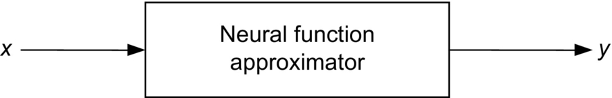
A conventional function approximator should give a good prediction of output data, when a system is presented with a new input data. A conventional function approximator uses a mathematical model of the system as shown in Fig. 37.1A. Sometimes, it is not possible to have an accurate mathematical model of the system, in such a case; mathematical model-free approximators are required, as shown in Fig. 37.1B. A conventional function approximator can easily be replaced by a neural-network-based function approximator.

37.2.2 Neural Function Approximator
The function ![]() is the function to be approximated, and x1,x2,x3,…xn are the n variables (n inputs), and the approximator uses the sum of nonlinear functions g1,g2,g3,g4,…,gi, where each of the g is nonlinear function of a single variable. Thus,
is the function to be approximated, and x1,x2,x3,…xn are the n variables (n inputs), and the approximator uses the sum of nonlinear functions g1,g2,g3,g4,…,gi, where each of the g is nonlinear function of a single variable. Thus,

where gi is a real and continuous nonlinear function that depends only on a single-variable zi. The output y can also be represented as

These equations can be represented by a network shown in Fig. 37.2. There are n input nodes in the input layer and M hidden nodes in the hidden layer.

Fig. 37.3 shows the schematic diagram of a neural approximation, and Fig. 37.4 shows the technique of its training. The error (e) between the desired nonlinear function (y) and the nonlinear function (ŷ) obtained by the neural estimator is the input to the learning algorithm for the artificial neural estimator. This type of learning is known as back propagation.

The output of a single neuron can be represented as

where fi is the activation function and bi is the bias. Fig. 37.5 shows a number of possible activation functions in a neuron. The simplest of all is the linear activation function, where the output varies linearly with the input but saturates at ![]() as shown with a large magnitude of the input. The most commonly used activation functions are nonlinear, continuously varying types between two asymptotic values 0 and 1 or
as shown with a large magnitude of the input. The most commonly used activation functions are nonlinear, continuously varying types between two asymptotic values 0 and 1 or ![]() and
and ![]() . These are, respectively, the sigmoidal function also called log-sigmoid and the hyperbolic tan function also called tan-sigmoid.
. These are, respectively, the sigmoidal function also called log-sigmoid and the hyperbolic tan function also called tan-sigmoid.

The learning process of an ANN is based on the training process. One of the most widely used training techniques is the error back-propagation technique, a scheme that is illustrated in Fig. 37.4. When this technique is employed, the ANN is provided with input and output training data, and the ANN configures its weights. The training process is then followed by supplying with the real input data, and the ANN then produces the required output data.
The total network error (sum of squared errors) can be expressed as

where E is the total error, P is the number of patterns in the training data, k is the number of outputs in the network, dkj is the target (desired) output for the pattern K, and ![]() is the jth output of the kth pattern. The minimization of the error can be arranged with different algorithms such as the gradient descent with momentum, Levenberg-Marquardt, reduced memory Levenberg-Marquardt, and Bayesian regularization.
is the jth output of the kth pattern. The minimization of the error can be arranged with different algorithms such as the gradient descent with momentum, Levenberg-Marquardt, reduced memory Levenberg-Marquardt, and Bayesian regularization.
37.3 ANN-Based Estimation in Induction Motor Drives
Artificial neural networks have found widespread use in function approximation. It has been shown that, theoretically, a three-layer ANN can approximate arbitrarily closely, any nonlinear function, provided that it is nonsingular. Some of the ANN-based estimators reported in the literature for rotor flux, torque, and rotor speed of induction motor drive are discussed in the following section.
37.3.1 Speed Estimation
In general, steady-state and transient analysis of induction motors is done using space-vector theory, with the mathematical model having the parameters of the motor. To estimate the various machine quantities such as stator- and rotor-flux linkages, rotor speed, and electromagnetic torque, the above mathematical model is normally used. However, these machine quantities could be estimated without the mathematical model by using an ANN. Here, no assumptions have to be made about any type of nonlinearity.
As an example, the rotor speed of an induction motor can be estimated from the direct and quadrature-axis stator voltages and currents in the stationary reference frame, as shown in Fig. 37.6. A three-layer feedforward neural network structure with ![]() (eight input, seven hidden, and one output) is used in this case. The input nodes were selected as equal to the number of input signals and the output nodes as equal to the number of output signals. The number of hidden layer neurons is generally taken as the mean of the input and output nodes. In this speed estimator ANN, seven hidden neurons were selected.
(eight input, seven hidden, and one output) is used in this case. The input nodes were selected as equal to the number of input signals and the output nodes as equal to the number of output signals. The number of hidden layer neurons is generally taken as the mean of the input and output nodes. In this speed estimator ANN, seven hidden neurons were selected.

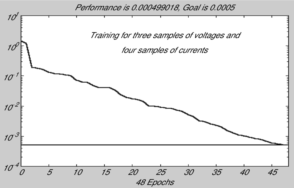
The results of an experiment conducted on a 1.1 kW, 415 V, 3 phase, 4 pole, 50 Hz induction motor is explained in this section. In order to investigate the case of speed estimation using ANN, a rotor-flux-oriented induction motor drive was set up in the laboratory, where the speed reference was changed in steps of 100 rpm and reversed every time the speed reached 1000 rpm. The load torque on the motor was kept constant at its full load rating. The stator voltages, stator currents, and rotor speed were measured for 5 s, and a data file was generated. The neural network was then trained using the trainlm algorithm with this data file. The training of the neural network converged after 48 epochs, and the error plot for this network training is shown in Fig. 37.7. The estimated speed was predicted with the trained neural network, and the result is shown in Fig. 37.8.
 network training for speed estimation.
The noisy data in the plot are the estimated speed, and the continuous line is the speed measured with the encoder. The speed estimation was found to fail for speeds <100 rpm. If the trained neural network has to predict the speed under the complete range of operation of the drive, the data for training the neural network also have to be taken for the whole range. From this example investigated, it was found that the off-line training of the neural network could not produce satisfactory results, and it can be concluded that these off-line methods are not most suitable for these applications.
Artificial neural networks were also used for the estimation of the rotor speed of an induction motor together with the help of induction motor dynamic model. Though the technique gives a fairly good estimate of the speed, this technique lies more in the adaptive control area than in neural networks. The speed is not obtained at the output of a neural network; instead, the magnitude of one of the weights corresponds to the speed. The four quadrant operation of the drive was not possible for speeds <500 rpm. The motor was not able to follow the speed reference during the reversal for speeds <500 rpm. The drive worked satisfactorily for speeds above 500 rpm. Even though this method does not fall into a true neural network estimator, the results achieved with this type of implementation were very good except for lower speeds.
Alternately, the estimated speed can be made available at the output of a neural network as shown in Fig. 37.9. This speed estimator used a three-layer neural network with five input nodes, one hidden layer, and one output layer to give the estimated speed ![]() as shown in Fig. 37.9. The three inputs to the ANN are a reference model flux λr⁎, an adjustable model flux
as shown in Fig. 37.9. The three inputs to the ANN are a reference model flux λr⁎, an adjustable model flux ![]() , and
, and ![]() , the time delayed estimated speed. The multilayer and recurrent structure of the network makes it robust to parameter variations and system noise. The main advantage of their ANN structure lies in the fact that they have used a recurrent structure that is robust to parameter variations and system noise. These authors were able to achieve a speed control error of 0.6% for a reference speed of 10 rpm. The speed control error dropped to 0.584% for a reference speed of 1000 rpm.
, the time delayed estimated speed. The multilayer and recurrent structure of the network makes it robust to parameter variations and system noise. The main advantage of their ANN structure lies in the fact that they have used a recurrent structure that is robust to parameter variations and system noise. These authors were able to achieve a speed control error of 0.6% for a reference speed of 10 rpm. The speed control error dropped to 0.584% for a reference speed of 1000 rpm.

37.3.2 Flux and Torque Estimation
The same principle as described in Section 37.3.1 can also be extended for simultaneous estimation of more quantities such as torque and stator flux. When more quantities or variables have to be estimated, the complex ANN has to implement a complex nonlinear mapping.
The four feedback signals required for a direct field-oriented induction motor drive can be estimated using ANNs. A ![]() multilayer network has been used for the estimation of the rotor-flux magnitude, the electromagnetic torque, and the sine/cosine of the rotor-flux angle. It has been demonstrated both by modeling and experimental results that the above estimated quantities were almost equal to the same quantities computed by a DSP-based estimator. Both the estimated torque and rotor-flux signals using neural network were found to have higher ripple content compared with the DSP-based estimated quantities. It could be concluded that a properly trained ANN could totally eliminate the machine model equations as evident from the results reported.
multilayer network has been used for the estimation of the rotor-flux magnitude, the electromagnetic torque, and the sine/cosine of the rotor-flux angle. It has been demonstrated both by modeling and experimental results that the above estimated quantities were almost equal to the same quantities computed by a DSP-based estimator. Both the estimated torque and rotor-flux signals using neural network were found to have higher ripple content compared with the DSP-based estimated quantities. It could be concluded that a properly trained ANN could totally eliminate the machine model equations as evident from the results reported.
In another application, an ANN with ![]() structure has been used to estimate the stator flux using the measured induction motor stator variable quantities. After successful training, the ANN was used in a direct field-oriented controlled drive. The rotor flux is computed from the stator flux estimate provided by the ANN and the stator current. This particular implementation also included an ANN-based decoupler which was used for the indirect field-oriented (IFO) drive. An ANN with a structure of
structure has been used to estimate the stator flux using the measured induction motor stator variable quantities. After successful training, the ANN was used in a direct field-oriented controlled drive. The rotor flux is computed from the stator flux estimate provided by the ANN and the stator current. This particular implementation also included an ANN-based decoupler which was used for the indirect field-oriented (IFO) drive. An ANN with a structure of ![]() was used for implementing the mapping between the flux and torque references and the stator current references. The estimated rotor flux using an ANN and a conventional FOC controller was shown to be equal. These authors have used experimental data for the ANN training, and thus, the effect of motor parameters was reduced. The authors were unable to use these estimated fluxes for controlling the induction motor in the experiment. The structure of the ANN used for this estimation is only that of a static ANN. It is preferable to have a dynamic neural network for this purpose.
was used for implementing the mapping between the flux and torque references and the stator current references. The estimated rotor flux using an ANN and a conventional FOC controller was shown to be equal. These authors have used experimental data for the ANN training, and thus, the effect of motor parameters was reduced. The authors were unable to use these estimated fluxes for controlling the induction motor in the experiment. The structure of the ANN used for this estimation is only that of a static ANN. It is preferable to have a dynamic neural network for this purpose.
37.3.3 Rotor Resistance Identification Using ANN
37.3.3.1 Off-Line Trained ANN
The artificial neural network can also be used for the rotor time constant adaptation in indirect field-oriented controlled drives. One of the implementation reported in the literature is shown in Fig. 37.10. There are five inputs to the Tr estimator, namely vdss,vqss,idss,iqss,ωr. The training signals are generated with step variations in rotor resistance for different torque reference Te⁎ and flux command λr⁎, and the final network is connected in the IFO controller as shown in Fig. 37.10. The rotor time constant was tracked by a proportional integral (PI) regulator that corrects any errors in the slip calculator. The output of this regulator is summed with that of the slip calculator, and the result constitutes the new slip command that is required to compensate for the rotor time constant variation. The major drawback of this scheme is that the final neural network is only an off-line trained neural network with a limited data file obtained from the modeling.

37.3.3.2 On-Line Trained ANN
The limitations of off-line trained ANN are overcome by using an online trained ANN configuration. The method discussed in this section has used an online trained ANN for adaptation of Rr of an induction motor in the RFOC induction motor drive. The error between the desired state variable of an induction motor and the actual state variable of a neural model is back propagated to adjust the weights of the neural model, so that the actual state variable tracks the desired value.
The principle of online estimation of rotor resistance (Rr) with multilayer feedforward artificial neural networks using online training has been described in “Multilayer feedforward ANN” section. This technique was then investigated with the help of modeling studies with a 1.1 kW squirrel-cage induction motor (SCIM), described in “Rotor resistance estimation for RFOC using ANN” section. The modeling results are presented in “Modeling results” section. In order to validate the modeling studies, modeling results were compared with those from an experimental setup with a SCIM under RFOC. These experimental results are presented in “Experimental results” section.
Multilayer feedforward ANN
Multilayer feedforward neural networks are regarded as universal approximations and have the capability to acquire nonlinear input-output relationships of a system by learning via the back-propagation algorithm. It should be possible that a simple two-layer feedforward neural network trained by the back-propagation technique can be employed in the rotor resistance identification. The modified technique using ANN proposed in this section can be implemented in real time so that the resistance updates are available instantaneously, and there is no convergence issues related to the learning algorithm. The two-layered neural network based on a back-propagation technique is used to estimate the rotor resistance. Two models of the state variable estimation are used; one provides the actual induction motor output, and the other one gives the neural model output. The total error between the desired and actual state variables is then back propagated as shown in Fig. 37.11, to adjust the weights of the neural model, so that the output of this model coincides with the actual output. When the training is completed, the weights of the neural network should correspond to the parameters in the actual motor.

Rotor resistance estimation for RFOC using ANN
The basic structure of an adaptive scheme described by Fig. 37.11 is extended for rotor resistance estimation of an induction motor as illustrated in Fig. 37.12. Two independent observers are used to estimate the rotor-flux vectors of the induction motor. If the rotor-flux linkages are estimated using the stator voltages and stator currents, they are referred to as voltage model, and if the rotor-flux linkages are estimated using the stator currents and rotor speed, they are referred to as current model.

The stator flux linkages based on the neural network model in Fig. 37.12 can be represented using Eq. (37.5), which is derived from the sample data models of the combined voltage and current model equations of the induction motor:
The neural network model represented by Eq. (37.5) is shown in Fig. 37.13, where W1, W2, and W3 represent the weights of the networks and X1, X2, and X3 are the three inputs to the network. If the network shown in Fig. 37.13 has to be used to estimate Rr, where W2 is already known, then W1 and W3 need to be updated.

The weights of the network, W1 and W3, are found from training, so as to minimize the cumulative error function E1:

The weight of the neural network W1 has to be adjusted using generalized delta rule.
To accelerate the convergence of the error back-propagation learning algorithm, the current weight adjustment has to be supplemented with a fraction of the most recent weight adjustment, as indicated in Eq. (37.7):
where α1 is a user-selected positive momentum constant and η1 is the training coefficient.
The rotor resistance Rr can now be calculated from W3 from Eq. (37.8) as follows:

Modeling results
A schematic diagram showing the implementation of a rotor resistance estimator in RFOC controller for induction motor is shown in Fig. 37.14. The stator voltages and currents are measured to estimate the rotor-flux linkages using the voltage model as shown in this figure. The inputs to the rotor resistance estimator (RRE) are the stator currents, the rotor-flux linkages ![]() ,
, ![]() , and the rotor speed ωr. The estimated rotor resistance
, and the rotor speed ωr. The estimated rotor resistance ![]() will then be used in the RFOC controllers for the flux model. The response of the drive together with the rotor resistance estimator OFF is shown in Fig. 37.15 for an abrupt change in Rr of motor, from 6.03 to 8.5 Ω at 0.8 s. The possible changes in the estimated motor torque Te, the rotor-flux linkage λrd with this estimator were noted.
will then be used in the RFOC controllers for the flux model. The response of the drive together with the rotor resistance estimator OFF is shown in Fig. 37.15 for an abrupt change in Rr of motor, from 6.03 to 8.5 Ω at 0.8 s. The possible changes in the estimated motor torque Te, the rotor-flux linkage λrd with this estimator were noted.


Subsequently, the results of the drive were looked at with RRE ON, so that the rotor resistance in the controller Rr′ was updated with the estimated rotor resistance ![]() as shown in Fig. 37.16. The estimated rotor resistance
as shown in Fig. 37.16. The estimated rotor resistance ![]() has converged to the rotor resistance of the motor Rr within 50 ms.
has converged to the rotor resistance of the motor Rr within 50 ms.

The response of the drive system with the RRE using ANN is also shown for a practical profile in load torque, speed, and change in Rr. The Rr was increased from 6.03 to 8.5 Ω over a period of 8 s, and the torque and rotor-flux linkage are shown in Fig. 37.17 when the RRE is OFF. For rapid reversals of the drive and variations in load torque, there are significant errors in rotor-flux linkages and thus errors in estimated torques. Subsequently, the RRE block was switched ON, and it can be observed that the rotor resistance estimator was tracking very well even during the worst dynamics in the motor speed and load torques as shown in Fig. 37.18. The estimated rotor resistance ![]() tracked the actual rotor resistance of the motor Rr throughout except that there was some small error during the reversal of the motor. The rotor-flux linkage λrd was found to remain constant at 1.0 Wb during this transient condition. The current iqs also remained constant as the torque is now perfectly decoupled.
tracked the actual rotor resistance of the motor Rr throughout except that there was some small error during the reversal of the motor. The rotor-flux linkage λrd was found to remain constant at 1.0 Wb during this transient condition. The current iqs also remained constant as the torque is now perfectly decoupled.


Experimental results
The practical implementation of the above rotor resistance estimation was found functioning very well in the experimental drive setup. The results of the Rr estimation obtained from the experiment is shown in Fig. 37.19 taken from a heat-run test conducted on an induction motor. As the RRE calculated, the rotor resistance using variables in stationary reference frame, the d-axis rotor-flux linkages of the current model (λdrim), the voltage model (λdrvm), and the neural model (λdrnm), taken at the end of heat run, is also recorded as shown in Fig. 37.20.


37.3.4 Stator Resistance Estimation Using ANN
In this section, the capability of a neural network has been deployed to have online estimator for stator resistance in an RFOC induction motor drive. The stator resistance observer was realized with a recurrent neural network with feedback loops trained using the standard back-propagation learning algorithm. Such architecture with recurrent neural network is known to be a more desirable approach, and the implementation reported in this section confirms this.
The d-axis stator current in the stationary reference frame in the discrete form can be represented using the voltage and current model equations of the induction motor:
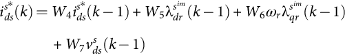

The weights W5, W6, and W7 are calculated using the induction motor parameters, the rotor speed ωr, and the sampling interval used in the estimator Ts.
The relationship between stator current and stator resistance is nonlinear that could be easily mapped using a neural network.
When this Eq. (37.9) is represented graphically, it resembles a recurrent neural network as shown in Fig. 37.21. The standard back-propagation learning rule can then be employed for training this neural network. The weight W4 is the result of training so as to minimize the cumulative error function E2:

To accelerate the convergence of the error back-propagation learning algorithm, the current weight adjustment is supplemented with a fraction of the most recent weight adjustment, as indicated in Eq. (37.11):
where η2 is the training coefficient and α2 is a user-selected positive momentum constant.
Following a similar procedure, the q-axis stator current of the induction motor can be estimated using the discrete form as shown in Eq. (37.12):

Equation (37.12) can be represented by a neural network as shown in Fig. 37.22. The weight W4 is updated with the training based on Eq. (37.12).

The stator resistance ![]() of the induction motor can now be calculated using Eq. (37.13) as follows:
of the induction motor can now be calculated using Eq. (37.13) as follows:

The stator resistance of an induction motor can be thus estimated from the stator current using the neural network system as indicated in Fig. 37.23.

37.3.4.1 Modeling Results of Stator Resistance Estimation Using ANN
The block diagram of a rotor-flux-oriented induction motor drive together with stator resistance identification is already shown in Fig. 37.14, where the stator resistance estimation is implemented by the stator resistance estimator (SRE) block.
The stator resistance estimation results are as shown in Fig. 37.24. It has three results (1) without both rotor and stator resistance estimators, (2) with only rotor resistance estimation, and (3) with both rotor and stator resistance estimations. As shown in the figure, both Rr and Rs were increased abruptly by 40% at 1.5 s. It can be seen that the estimated stator resistance ![]() converges to
converges to ![]() within 200 ms. It can be noted from this figure that the convergence of the stator resistance estimation is not affected by the convergence of the rotor resistance estimator.
within 200 ms. It can be noted from this figure that the convergence of the stator resistance estimation is not affected by the convergence of the rotor resistance estimator.

37.3.4.2 Experimental Results of Stator Resistance Estimation Using ANN
The stator resistance estimation algorithm was tested together with the rotor-flux-oriented induction motor drive of Fig. 37.14 implemented in the laboratory. To test the stator resistance estimation, an additional 3.4 Ω per phase was added in series with the induction motor stator, with the motor running at 1000 rev/min and with a load torque of 7.4 Nm.
The estimated stator resistance together with the actual stator resistance is shown in Fig. 37.25. The estimated stator resistance converges to 9.4 Ω within <200 ms.

Fig. 37.26 shows both the measured d-axis stator current and the one estimated by the neural network model. The neural network model output ![]() follows the measured values idss(k), due to the online training of the neural network.
follows the measured values idss(k), due to the online training of the neural network.

37.4 ANN-Based Controls in Motor Drives
37.4.1 Induction Motor Current Control
Another application of ANN is to identify and control the stator current of an induction motor. In one study, Burton et al. have used a current control strategy outlined by Wishart and Harley to train an ANN to control the induction motor stator currents. They have used a training algorithm named random weight change (RWC) that is reported to be slightly faster than back propagation. In RWC algorithm, the weights are perturbed by a fixed step size and a random sign. This is done for fixed number of trials, and after each trial, the error with the desired output is computed. Finally, the set of weight changes that result in the least error are chosen, and the whole process is repeated until convergence is reached. The modeling results reported in this scheme was excellent. Later, Burton et al. presented their practical implementation of this proposed stator current controller with a transputer controller card.
37.4.2 Induction Motor Control
Narendra and Parthasarathy proposed methods for identification and control of dynamic systems using ANNs. Wishart and Harley used the above basic principles to identify and control induction machines. A block diagram of the control scheme is shown in Fig. 37.27. For the induction motor, the nonlinear autoregressive moving average with exogenous input (NARMAX) model for the stationary frame stator current is derived and used for the identification of electromagnetic model. In its general form, the NARMAX model represents a system in terms of its delayed inputs and outputs. Random steps in the stator voltage are given for the purpose of identification. The neural network used is of the multilayer back-propagation type, and a quantity based on the rotor time constant is also computed as an extra weight. As opposed to the regular ANN architecture, this ANN has nonlinearity in the output layer, and the weighted sum of the inputs is used as the output. This gives an estimate of the rotor time constant and makes the system robust against variation of the parameters. Once, the identification is over, the ANN is used for current control. The stator currents predicted by the ANN are used to compute the input voltage for the induction motor, and the ANN output is made to track the reference currents by back propagating the error.

The rotor speed is also controlled in this system by identifying a NARMAX model for the speed increment rather than the absolute value of speed. To simplify the NARMAX model, the load torque is assumed to be a function of the motor speed, as is the case in a fan or pump type of load. For the current control case, the relationship between the control variable (voltage) and the controlled quantity (current) was linear. In the speed control case, this relationship is nonlinear, thus necessitating two ANNs, one for identification of speed and the other for control.
The identification ANN (Ni) predicts the value for the speed increment, which is compared with the actual speed increment, and the error (ɛi) is back propagated through the ANN. A PI controller is used for basic speed control, and the control ANN (Nc) produces the slip frequency, and the difference between the desired speed increment and actual speed increment (ɛc) is back propagated through the ANN. The induction motor drive therefore employs three ANNs as shown in Fig. 37.28.

37.4.3 Efficiency Optimization in Electric Drives
The efficiency improvement of induction motor drives via flux control can be classified into three groups: precomputed flux programs, real-time computation of losses, and online input-output efficiency optimization control. All of these methods target choosing a value of the motor excitation that optimizes the motor-converter losses. The main requirement of an input-output optimization is to achieve the flux optimization in a minimum number of search steps. A constant search step may take too long if the step is too small, or it may bypass the minimum power input if the step is too large. For each mechanical operating point of the motor, it is possible to find a combination of rotor-flux linkage and torque producing current iq at which the dc-link power Pdc to the drive system is minimum.
One of the possible ANN efficiency optimizers reported is shown in Fig. 37.29. An ANN-based search algorithm is employed to operate as an efficiency optimizer. The inputs to the system are the dc power fed into the drive system at instant k and the change in the control variable at the previous instant ![]() . The only output is the actual change in control variable Δc(k). Appropriate scaling from engineering units to the normalized interval [−1, 1] are implemented by the input and output interfaces, input scaling (IS), and output scaling (OS). The speed signal is used to generate the reference flux C(k)0 corresponding to each speed. The mechanical steady state is detected by applying a moving average filtering to the speed variation Δωm. The ANN efficiency optimizer is enabled only during the mechanical steady state.
. The only output is the actual change in control variable Δc(k). Appropriate scaling from engineering units to the normalized interval [−1, 1] are implemented by the input and output interfaces, input scaling (IS), and output scaling (OS). The speed signal is used to generate the reference flux C(k)0 corresponding to each speed. The mechanical steady state is detected by applying a moving average filtering to the speed variation Δωm. The ANN efficiency optimizer is enabled only during the mechanical steady state.

37.5 ANN-Based Controls in Power Converters
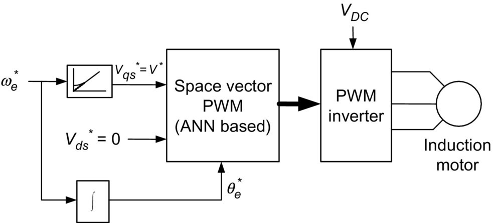
A feedforward ANN can implement a nonlinear input-output mapping. A feedforward carrier-based pulse-width modulation (PWM) technique, such as space-vector modulator (SVM), can be looked at as a nonlinear mapping where the command phase voltages are sampled at the input and the corresponding pulse-width patterns are established at the output. Fig. 37.30 shows the block diagram of an open-loop V/f-controlled induction motor drive incorporating the proposed ANN-based SVM controller. The command voltage ![]() is generated from the frequency or speed command, and the angle command θe⁎ is obtained by integrating the frequency, as shown. The output of the modulator generates the PWM patterns for the inverter switches.
is generated from the frequency or speed command, and the angle command θe⁎ is obtained by integrating the frequency, as shown. The output of the modulator generates the PWM patterns for the inverter switches.
The ANN can be conveniently trained off-line with the data generated by calculation of the SVM algorithm. The ANN has inherent learning capability that can give improved precision by interpolation unlike the standard lookup table method. Fig. 37.31 shows such an SVM that can operate during both undermodulation and overmodulation regions linearly extending smoothly up to a square wave. The SVM is implemented using two subnets: angle subnet and amplitude subnet. The subnets use a multiplayer perceptron-type network with sigmoidal-type transfer function. The bias is not shown in the figure. The composite network uses two neurons at the input, 20 neurons in the hidden layer, and four output neurons. The input signal to the angle subnet is θe angle that is normalized, and then pulse-width functions at unit amplitude are solved (or mapped) at the output for three phases, as indicated. The amplitude subnet implements the f(V⁎) function. The digital words corresponding to the turn-on time are generated by multiplying the angle subnet output with that of the amplitude subnet and then adding the Ts/4 bias signal, as shown. The PWM signals are then generated using a single timer. The angle subnet is trained with an angle interval of 2.16 degrees in the range of 0–360 degrees. Due to learning or interpolation capability, both the subnets will operate higher signal resolution. A sampling interval Ts of 50μs corresponds to a switching frequency of 20 kHz and a 100μs that corresponds to 10 kHz.

 for PWM wave synthesis.