Predictive Control of Power Electronic Converters
Sertac Bayhan Texas A&M University at Qatar, Doha, Qatar
Gazi University, Ankara, Turkey
Haitham Abu-Rub Texas A&M University at Qatar, Doha, Qatar
Abstract
The importance of advanced control techniques in the power electronics is increasing day by day due to the requirement of the new developed standards and regulations. Model predictive control (MPC), one of the most advanced control techniques, has been at the forefront in the control of power electronic converters in recent years because of its significant advantages over the linear control techniques. In this chapter, the use of model predictive control in power electronic converters is elaborated. Firstly, the theory and operational principle of predictive control are presented. After that, predictive control types including deadbeat control, hysteresis based, trajectory based, and model predictive control are summarized. Then, the implementation of MPC for power electronic converters is explained step by step. Traditional three-phase voltage source inverter is tackled to explain the MPC idea for power converters. Furthermore, two case studies are presented in order to verify MPC technique for different power converter topologies.
Keywords
Digital control; Model predictive control; Cost function; Multivariable control systems; Power converters
Acknowledgment
This chapter was made possible by NPRP grant No. NPRP-EP X-033-2-007 from the Qatar National Research Fund (a member of Qatar Foundation). The statements made herein are solely the responsibility of the authors.
40.1 Introduction
In recent years, power electronic converters have been involved in many applications from industrial level (motor drives, renewable energy technologies, etc.) to home level (PCs, home appliances, etc.). Therefore, the widespread use of power electronic converters puts their control requirements at the forefront. Traditionally, the control techniques in such converters are supposed to have good dynamic response and high reference tracking accuracy. In addition to these requirements, modern control methods should take into account some technical specifications and constraints to meet national and international standards and grid codes. Although these requirements often can be met with the hardware modifications, this results in extra cost. Thus, this shift in trend has driven the development of more advanced control methods, which should fulfill many control objectives at the same time [1].
One of these control methods is predictive control that has appeared as an attractive solution for the control of power converters due to its fast dynamic response and increased control accuracy [1–3]. Originally, this method was introduced in the process industry, but a very innovative and early paper applied predictive control for power electronics [4]. The main approach is based on the computation of the future system dynamic to calculate optimal actuation variables. Therefore, this technique requires a high amount of calculations, compared with classic control schemes; fortunately, parallel computational capable microprocessors are available in the current market to make possible the implementation of predictive control [5].
Furthermore, predictive control brings considerable benefits to power electronics systems. First of all, concepts are intuitive and easy to understand and implement, it can be applied to a variety of systems, it allows for nonlinearities and constraints to be incorporated into the control law in a straightforward manner, a multivariable case can be considered, and the resulting controller is easy to implement. However, the method requires a high amount of calculations, compared with a classic control scheme; however, the fast microprocessors available today make possible the implementation of predictive control. Generally, the quality of the controller depends on the quality of the model [6].
The aim of this chapter is to provide a comprehensive overview of predictive control and to illustrate its use in power electronic converters. It starts with an overview of predictive control theory. Then, predictive control types are presented along with a description of advantages and disadvantages of each type of predictive control. After that, implementation of MPC for power electronic converters is described. Finally, two case studies are given with simulation and experimental results.
40.2 Theory of Predictive Control
The main idea of the predictive control can be roughly explained as follows: it uses a discrete-time model of the system to forecast the future behavior of the controlled parameters during a certain time window called a receding horizon. A basic block diagram of this control technique is given in Fig. 40.1 [7]. It can be seen that predictive control consists of two main blocks: model and optimizer. To predict behavior of the system at the next sampling time, the system discrete-time model is used. Then, the future error between predicted output and the reference value is minimized by using predefined cost function in the optimizer. To sum up briefly, the basic idea of MPC can be explained as follows:

• A discrete-time model of the system should be obtained in order to predict system output at the next sampling instant.
• To obtain the optimal actuation, the cost function is used in the optimizer block.
The system prediction model can be defined as state space model as follows:
where x(k+1), u(k), and y(k) are the state variable vector, the input vector, and the output vector, respectively. Furthermore, A is the system matrix, B is the control matrix, C is the output matrix, and D is the feedthrough matrix. The prediction model can be obtained by combining N equations at k+1th through k+Nth instants as follows [8]:

This prediction model can be expressed as
A cost function (g) is needed to be determined to select an optimal actuation in the next sampling time. Since the objective of the controller is to guide the system state toward zero from any given initial conditions, the cost function can be defined as follows:
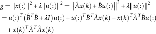
where λ is a weighting factor. Taking the derivative of the cost function with respect to u(:) and setting it to zero, one obtains
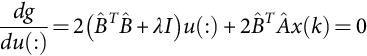
whose solution is
Following the fundamental concept behind predictive control, only the first vector from the array of the optimally predicted future control inputs in Eq. (40.8) is utilized. Hence, the control input vector at the kth time instant can be found to be
Fig. 40.2 illustrates the working principle of predictive control. The future values of the system states are predicted until a predefined horizon in time k+N using the system model and the available measured data until time k. The sequence of the optimal actuation is calculated by minimizing the cost function. This process is repeated taking into account the new measured data for each sampling time [9].

40.3 Types of Predictive Control
The classification of predictive control in power electronic converters can be divided into four main categories, as shown in Fig. 40.3 [10]. The deadbeat control consists of determining which input signal must be applied to the system to ensure the output reaches steady state in the smallest number of time steps. Although deadbeat control requires a modulator, it provides constant switching frequency and requires low computation burden to be implemented in digital platforms. The optimization criterion in the hysteresis-based predictive control is to keep the controlled variable within the boundaries of a hysteresis area, while in the trajectory based, the variables are forced to follow a predefined trajectory. Furthermore, hysteresis-based and trajectory-based predictive controls can be accepted as direct control technique, which means that it doesn’t need modulator stage; however, switching frequency is variable. Model predictive control (MPC), which is the most significant predictive control technique for power electronic converters among the others, can be classified in two categories: continuous control set MPC (CCS-MPC) and finite control set MPC (FCS-MPC). CCS-MPC requires a modulator to generate the switching states, while in FCS-MPC, the switching state can be generated without modulator stage. In FCS-MPC approach, to solve the optimization problem, the power converters' finite number of switching states is used. To do that, a discrete-time model of the system should be employed to predict the future behavior of the system. Then, an optimal control actuation is selected by the predefined cost function. Although FCS-MPC can generate switching signals without a modulator, switching frequency is variable.
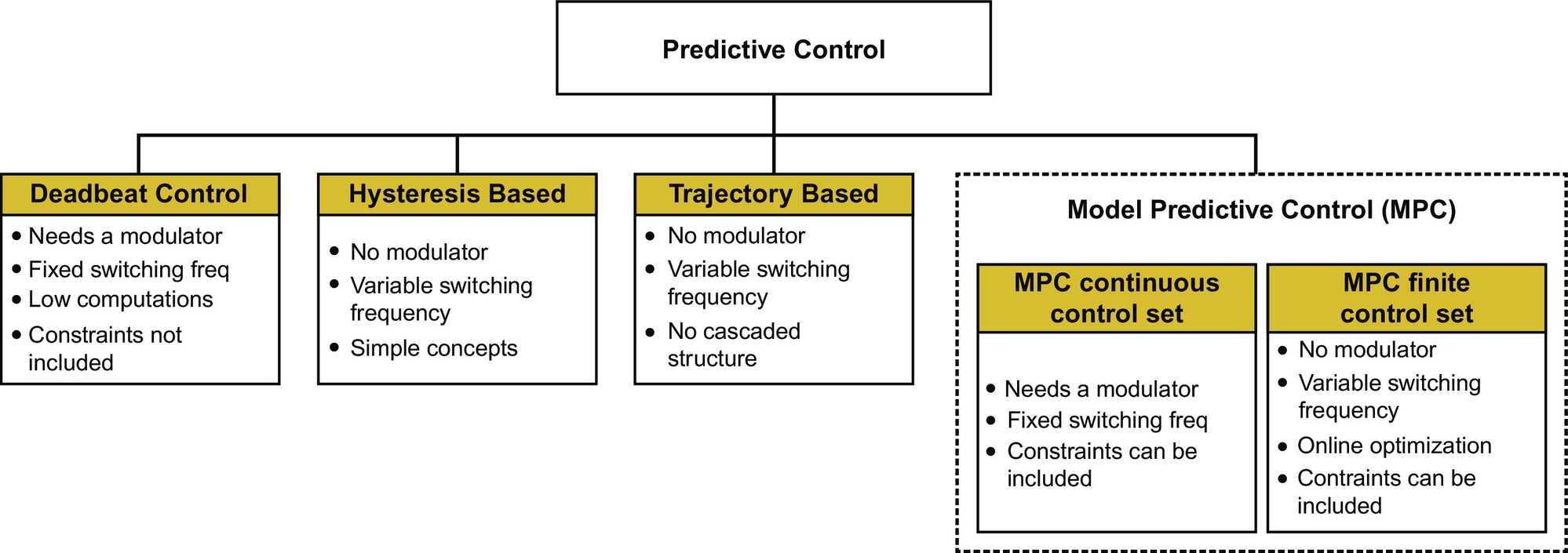
Simplicity and easy implementation concept are the most important advantages of predictive control. Using predictive control technique also allows avoiding the cascaded control structure, which results in fast dynamic response in control. Furthermore, some constraints can be included in the control in order to improve the system performance. Although these advantages can be easily implemented in some predictive control techniques such as MPC, but it is very difficult to add in deadbeat control.
40.4 Model Predictive Control for Power Electronics
In this subsection, the implementation of MPC for power electronic converters will be explained step by step. Although this technique is suitable for all power electronic converters, traditional three-phase three-leg voltage source inverter (VSI) will be taken as an example to explain the MPC idea for power converters.
The block diagram of the MPC for three-phase VSI is shown in Fig. 40.4. This control technique can be summarized by the following steps:
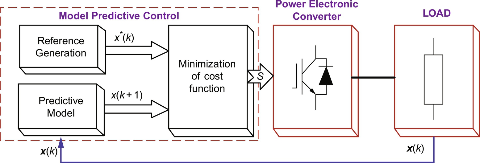
• Build a model of the converter and determine the possible switching states.
• Build a model of the load for the predictive model.
• Define a cost function to minimize the error.
40.4.1 Converter Model
The traditional three-phase VSI with RL load and VSI equivalent circuits are shown in Fig. 40.5 [11]. As shown, each leg can be represented as a dual-way switch, so only one switch can be active simultaneously in the same leg in order to avoid short circuit. The switching states Sa, Sb, Sc are controlled as follows:
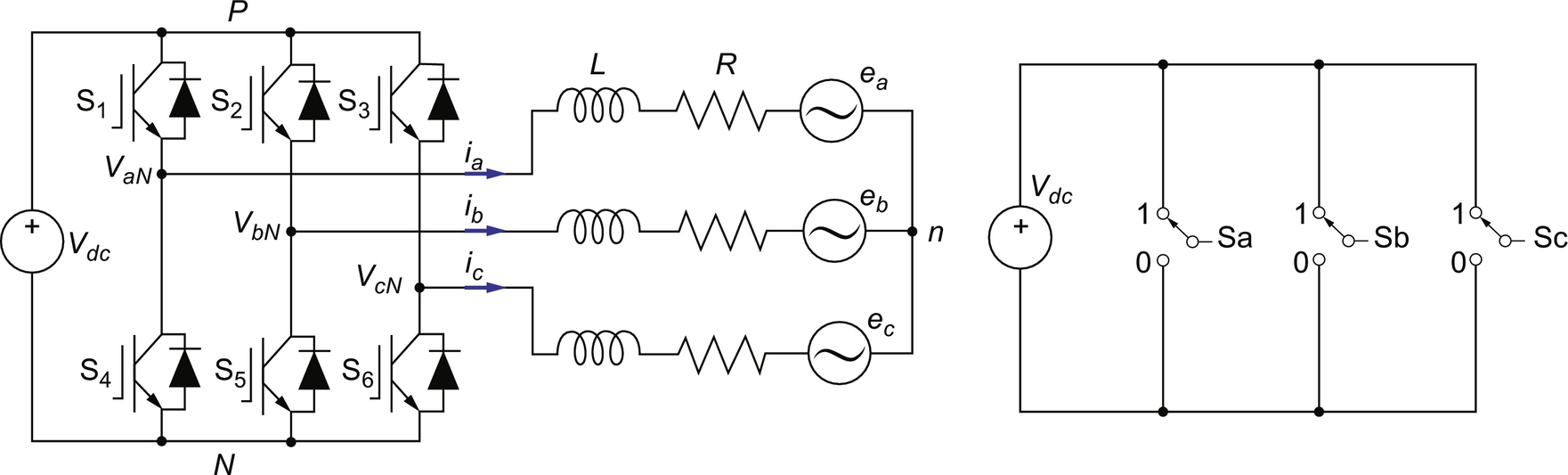


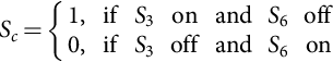
These switching states can be expressed as
where a is called as a unitary vector and is equal to ej2π/3. Finally, the inverter output voltage vector can be defined as a function of the switching state vector S by
where Vdc is the dc-link voltage.
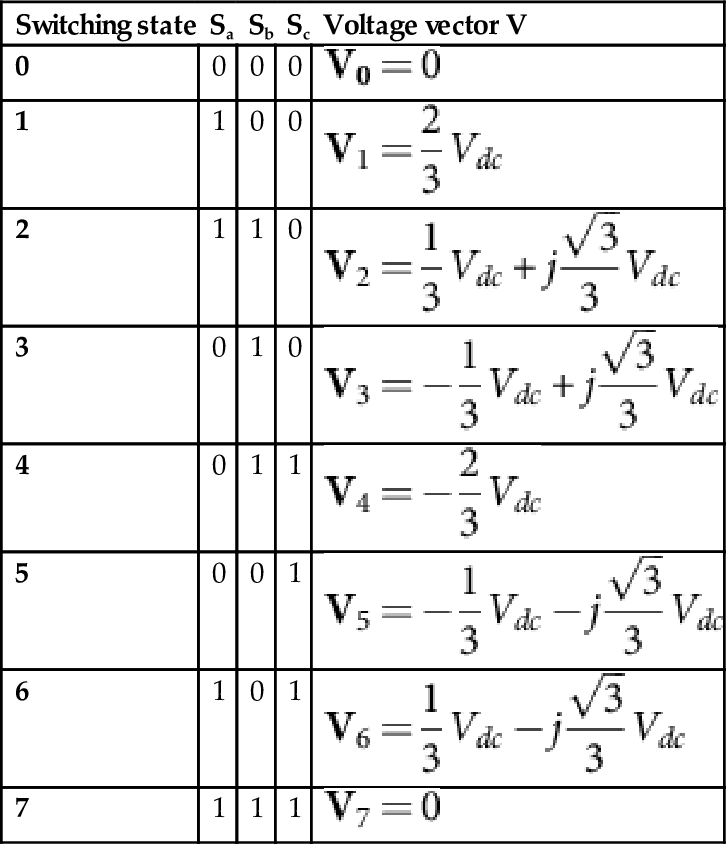
Considering all the possible combinations of the switches (Sa, Sb, Sc), eight switching states and consequently eight voltage vectors can be obtained, as shown in Fig. 40.6. Six of these vectors (v1–v6) are defined as active vectors, while the other two (v0, v7) are defined as zero vector. Consequently, seven different voltage vectors are obtained as shown in Fig. 40.6.

40.4.2 Discrete-Time Model of Load for Prediction
The equivalent circuit of the three-phase VSI with RL load is shown in Fig. 40.7. The continuous-time model of the system can be expressed as
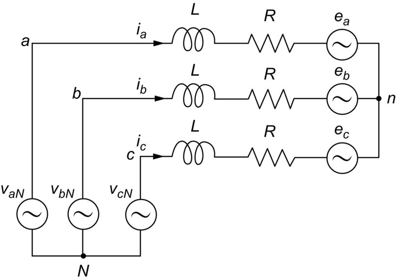
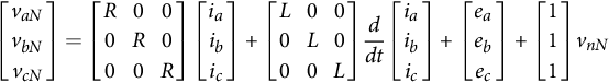
where R and L are the load resistance and the load inductance, respectively. This equation can be simplified as

where v is inverter output voltage vector, i is the load current vector, and e the load back-emf vector. The derivative of the output current vector can be obtained from

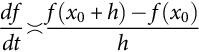
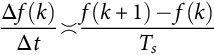
To use mathematical equations in the prediction model, discrete-time equations of the system must be obtained from continuous-time equations. To do that, the general structure of forward-difference Euler equation (40.18) can be used in order to compute the differential equations of the output current [12,13]:
To estimate these variables in the next sampling time, the discretization equation can be defined as
The continuous-time expression for the iabc is given in (40.17). By substituting (40.19) into (40.17), the discrete-time model of the iabc can be obtained as
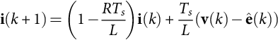
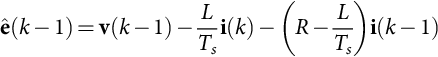
where i(k+1) is the predicted output current vector at the next sampling time and ê(k) denotes the estimated back emf that can be calculated from (40.16) considering the measurements of the load voltage and current with the following expression;
where ![]() is the estimated value of
is the estimated value of ![]() .
.
40.4.3 Cost Function Optimization
The objective of the cost function is to minimize the error between the reference currents (iabc*(k)) and the predicted output currents (![]() ) at the next sampling time. The cost function can be expressed in orthogonal coordinates as
) at the next sampling time. The cost function can be expressed in orthogonal coordinates as

where ![]() and
and ![]() are the real and imaginary parts of the predicted load current vector, while
are the real and imaginary parts of the predicted load current vector, while ![]() and
and ![]() are the real and imaginary parts of the reference load current. To simplify the analysis, it is assumed that the reference current does not change immediately in one sampling time. Thus,
are the real and imaginary parts of the reference load current. To simplify the analysis, it is assumed that the reference current does not change immediately in one sampling time. Thus, ![]() can be considered. On the other hand, this may introduce a one sample delay in the reference tracking, which can be neglected in high sampling frequency conditions. In general, the reference current is generated from an external control loop, for example, maximum power point tracking control loop.
can be considered. On the other hand, this may introduce a one sample delay in the reference tracking, which can be neglected in high sampling frequency conditions. In general, the reference current is generated from an external control loop, for example, maximum power point tracking control loop.
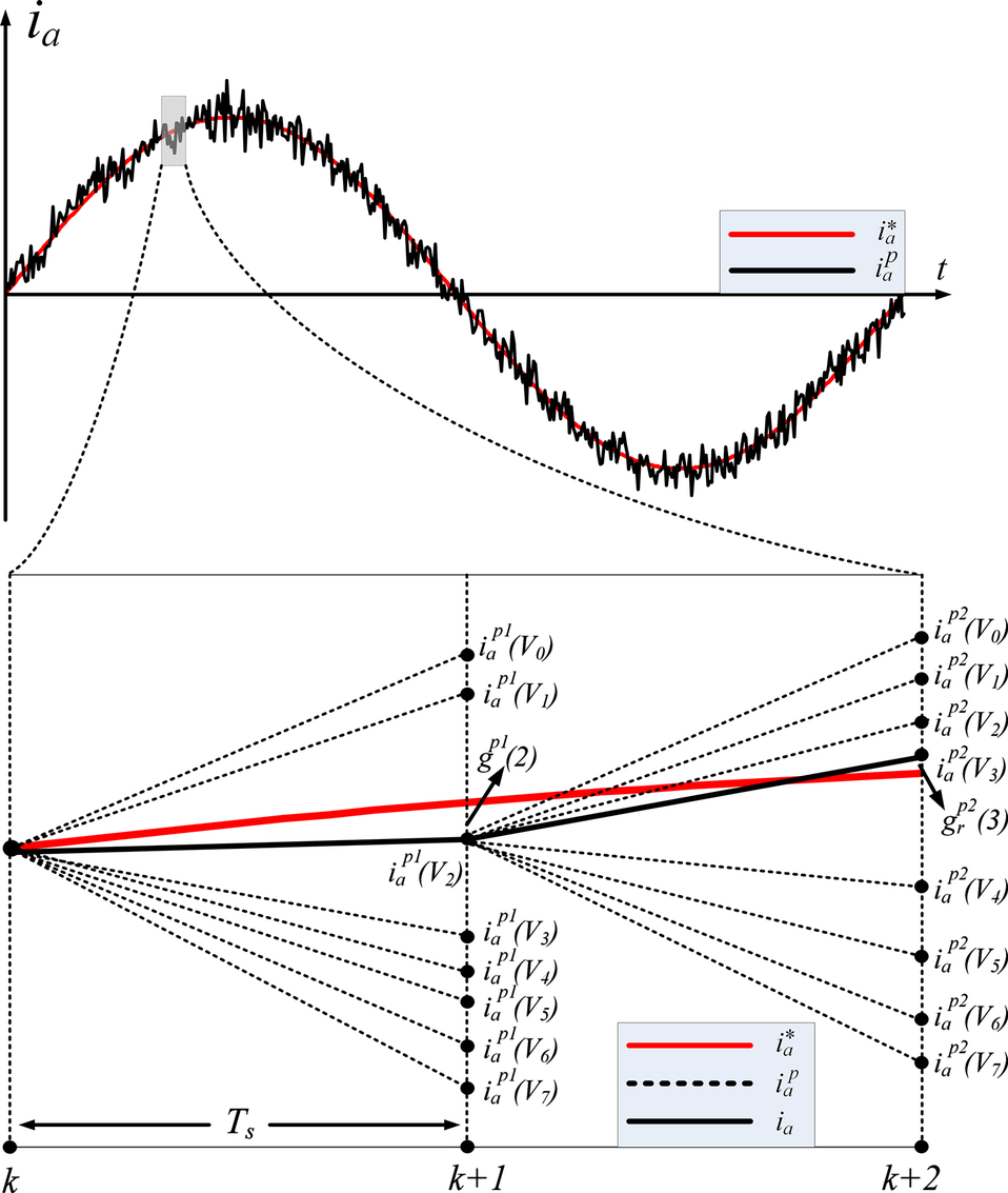
The sketch map of the reference and predicted rotor currents is shown in Fig. 40.8 to illustrate how the proposed MPC strategy works. Here, the measured output current ia(k) and voltage vectors v0-7, which are given in Table 40.1, have been evaluated together to estimate the future output current ia(k+1) values. As shown in Fig. 40.8, there are eight different predicted rotor current values at time k+1 and k+2. However, it can be seen from the figure that only v2 and v3 voltage vectors minimize the error of the output current at k+1 and k+2 instants, respectively. Thus, voltage vectors that minimize the cost function g are v2 at k+1 and v3 at k+2 are selected. In other words, corresponding voltage vector at each sample time is determined by the cost function according to the minimum error or distance between reference and predicted currents. As a result, it can be shown that v2 and v3 voltage vectors produce the lowest value of the cost function at k+1 and k+2 instants, respectively.
40.4.4 Control Algorithm
The MPC algorithm can be implemented as a “for” loop to predict future behavior of the system output, minimize the error between the reference and predicted output using predefined cost function, and store the index value of the corresponding switching state [14,15]. The flowchart of the MPC algorithm is given in Fig. 40.9. The control algorithm can be summarized by the following steps:
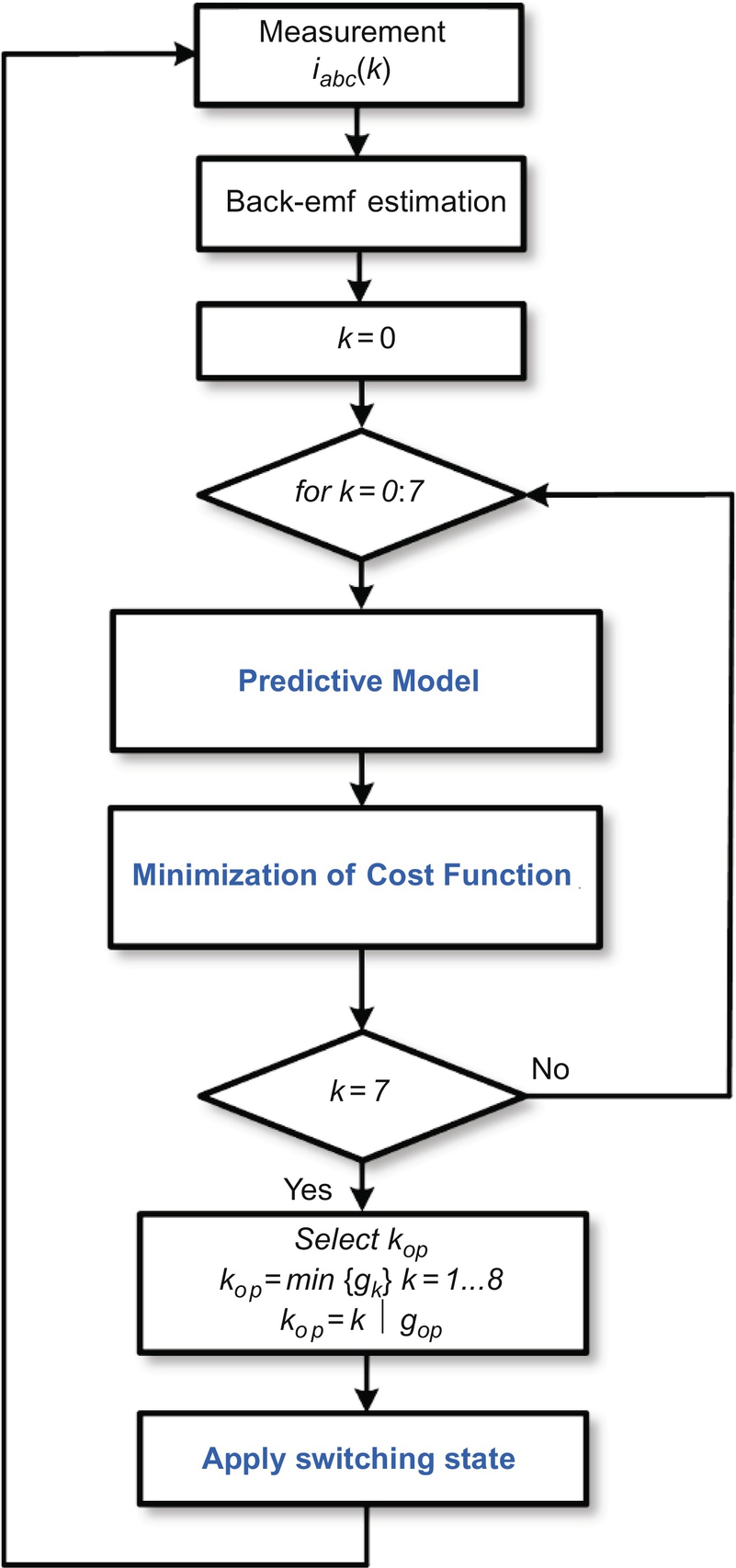
• Measure the output currents (iabc).
• Estimate the back emf using Eq. (40.21).
• These measured and estimated values are used to predict output currents using the predictive model in Eq.(40.20).
• All predictions are evaluated using the predefined cost function.
• The optimal switching state that corresponds to the optimal voltage vector that minimizes the cost function is selected to be applied at the next sampling time.
40.5 MPC Applications in Power Electronic
40.5.1 Three-Level Neutral-Point-Clamped Inverter
Motivated by the aforementioned advantages of MPC and considering the multiobjective control requirements of neutral-point-clamped (NPC) inverter, in this subsection, MPC-based control technique for three-phase NPC inverter is presented. Here, two parameters, the output current and the capacitor voltages, are controlled by the MPC technique. Thus, multiobjective control requirement is solved with simple technique.
A. System Model
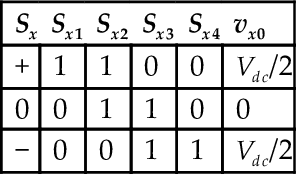
The used three-phase NPC inverter topology is illustrated in Fig. 40.10. Each leg of the inverter consists of four power switches with two diodes that allow the output terminal to be connected to the middle point of the split dc-link capacitors. This circuit configuration allows to generate three voltage levels at the output of the inverter according to the neutral point. The switching combinations are given in Table 40.2 [16]. Switching state variable Sx represents the switching state of phase x, with x=a, b, c, and it has three possible values denoted by positive, zero, and negative that represent the switching combinations that generate Vdc/2, 0, and−Vdc/2, respectively, at the output of the inverter phase.
The NPC inverter applies to the load 19 voltage vectors, which are generated from 27 switching states, as shown in Fig. 40.11 [16]. In addition to these switching states, for this application, one extra switching state is required to ensure shoot-through state. During this state, dc link must be short-circuited by single or multiple inverter legs.
The continuous-time expression for the output current (io) can be described by the following equation:


Table 40.2
Switching states for one phase of the NPC inverter
| Sx | Sx1 | Sx2 | Sx3 | Sx4 | vx0 |
| + | 1 | 1 | 0 | 0 | Vdc/2 |
| 0 | 0 | 1 | 1 | 0 | 0 |
| − | 0 | 0 | 1 | 1 | Vdc/2 |

where R and L are the load resistance and inductance, respectively, v is the voltage vector generated by the inverter, e is the electromotive force of the load, and i is the load current vector. These vectors are defined as

where ![]() .
.
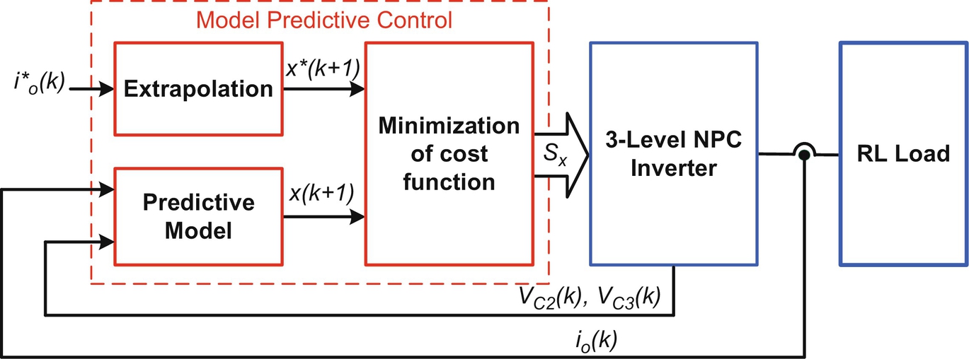
B. MPC-based control algorithm
The proposed MPC algorithm applied to the three-level NPC inverter is shown in Fig. 40.12. To predict the output current (io) and the capacitor voltages (vC1 and vC2) at the next sampling time, discrete-time model of the inverter must be defined. One way to obtain discrete-time models is to use the forward-difference Euler equation due to its simplicity. The derivative form dx(t)/dt is approximated by
where Ts is the sampling time and x is one of the control parameters such as i and vc12.
By substituting (40.23) into (40.25), the discrete-time model of the output current vector is

where i (k+1) is the predicted output current vector at the next sampling time.
The current prediction in (40.26) also requires an estimation of the future load back EMF e (k+1). It can be estimated by using a second-order extrapolation from present and past values. From (40.25) and the output voltage and current, resulting in the following expression:
where ê(k) is the estimated value of e(k).
Furthermore, the discrete-time equations of the capacitor voltage can be expressed by using (40.25):

where vC12(k+1) is the predicted capacitor voltages, at the next sampling time.
To use reference value in the cost function, this value must be extrapolated to k+1 instant. To do that, Lagrange's extrapolation can be used [17]. Once the extrapolated reference values obtained, they are applied in the cost function optimization block as can be seen in Fig. 40.12. To handle the desired control objectives, two terms are required to be defined in the cost function. The terms are responsible for minimizing the error between the reference and predicted values. The defined cost function is

where λ is the weighting factor.
C. Simulation Results
The simulation of the proposed system was performed using Matlab/Simulink environment. The NPC inverter topology, shown in Fig. 40.10, is used in the simulation. The parameters used in the simulation are summarized in Table 40.3.
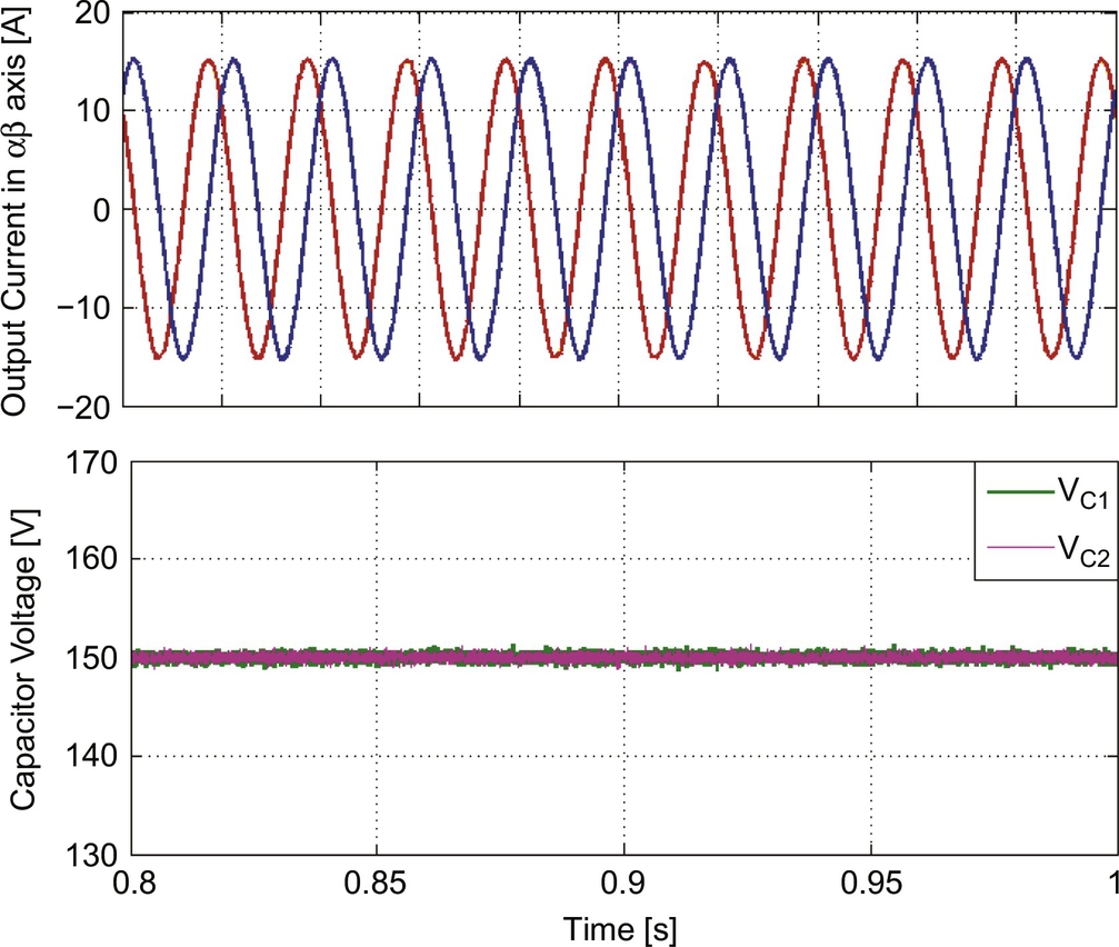
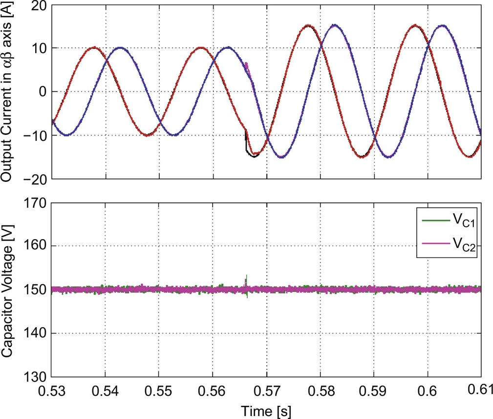
The simulation result of steady-state analysis is shown in Fig. 40.13. The reference output currents track their references with high accuracy, while the dc-link voltage is kept balanced by the MPC. Fig. 40.14 shows the simulation result of the transient response of the proposed control technique. The output reference current is step changed from 10 to 15 A. It can be seen that the dc-link voltage remains balanced at 150 V, with small deviations during the transient.
40.5.2 33-Level Input Switched Inverter
The control of multilevel inverters (MIs) is quite challenging and requires a flexible approach to success multiple control objectives. The MPC technique is extremely effective to control MIs due to its considerable advantages over the traditional linear controller. This subsection presents MPC technique for 33-level input switched multilevel inverter (ISMI) to verify MPC's effectiveness in the high-level MI topologies.
A. Overview of the ISMI
The circuit diagram of the single-phase 33-level ISMI with PV generation system is shown in Fig. 40.15 [18]. The ISMI topology has two stages, consisting of the multilevel module and H-bridge inverter. Output voltage level of this topology is given by Nlevel=2n+1, where n represents the number of power legs. In order to obtain 33 voltage level, n should be 16 for this application.
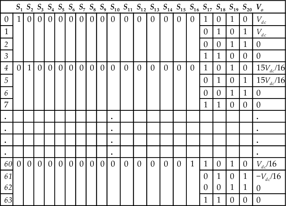
In the first stage, each leg includes two power switches that allow bidirectional current flow. Sixteen capacitors are also employed to divide the dc-link voltage equally to Vdc/16, as seen in Fig. 40.15. The bidirectional power switches of each leg should be gated on sequentially to obtain desired voltage level. It is noticeable that more than one leg switches cannot be turned on at the same time because input dc source would be short circuit. Moreover, the switching state of the multilevel module is determined by the output current direction and the voltage level of the multilevel module. For example, when the first leg (S1ab) is turned on and other legs are turned off, the output voltage (vx) of the multilevel module is Vdc, the current flows through S1a and D1b. The proposed ISMI has 64 switching states that produce thirty-three voltage levels. However, it should be noted that the voltage level of the multilevel module is only 16 positive levels. Therefore, to obtain positive and negative levels, the traditional H-bridge inverter is employed in the second stage of this topology, as seen in Fig. 40.15. The H-bridge inverter provides voltage gains, which are +1, 0, −1, to ensure positive, zero, and negative voltage on the output. The switching states of 33-level ISMI are given in Table 40.4.
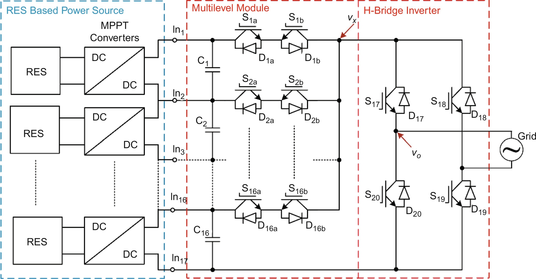
Table 40.4
Switching states of 33-level ISMI
| S1 | S2 | S3 | S4 | S5 | S6 | S7 | S8 | S9 | S10 | S11 | S12 | S13 | S14 | S15 | S16 | S17 | S18 | S19 | S20 | Vo | |
| 0 | 1 | 0 | 0 | 0 | 0 | 0 | 0 | 0 | 0 | 0 | 0 | 0 | 0 | 0 | 0 | 0 | 1 | 0 | 1 | 0 | Vdc |
| 1 | 0 | 1 | 0 | 1 | Vdc | ||||||||||||||||
| 2 | 0 | 0 | 1 | 1 | 0 | ||||||||||||||||
| 3 | 1 | 1 | 0 | 0 | 0 | ||||||||||||||||
| 4 | 0 | 1 | 0 | 0 | 0 | 0 | 0 | 0 | 0 | 0 | 0 | 0 | 0 | 0 | 0 | 0 | 1 | 0 | 1 | 0 | 15Vdc/16 |
| 5 | 0 | 1 | 0 | 1 | 15Vdc/16 | ||||||||||||||||
| 6 | 0 | 0 | 1 | 1 | 0 | ||||||||||||||||
| 7 | 1 | 1 | 0 | 0 | 0 | ||||||||||||||||
| . | . | . | |||||||||||||||||||
| . | . | . | |||||||||||||||||||
| . | . | . | |||||||||||||||||||
| . | . | . | |||||||||||||||||||
| 60 | 0 | 0 | 0 | 0 | 0 | 0 | 0 | 0 | 0 | 0 | 0 | 0 | 0 | 0 | 0 | 1 | 1 | 0 | 1 | 0 | Vdc/16 |
| 61 62 |
0 0 |
1 0 |
0 1 |
1 1 |
−Vdc/16 0 | ||||||||||||||||
| 63 | 1 | 1 | 0 | 0 | 0 |
B. MPC-based control algorithm for 33-level ISMI
The block diagram of the MPC strategy applied to the current control for the 33-level grid-connected ISMI is shown in Fig. 40.16. The predictive model of the system needs output current information in order to generate reference current. Grid phase angle information is also required to generate reference current in same phase with the grid voltage. In this case, the output current io(k) and the grid voltage vg(k) need to be measured. The phase angle (θe) of the reference current is obtained from PLL block. Thus, generated reference current will be in same phase and frequency with the grid voltage.
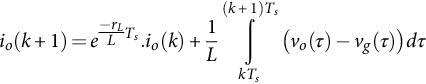
To control the output current (io) of the ISMI, a discrete-time model of the io must be defined. To do that, the averaged model of the system, which is defined in (40.30), can be used:

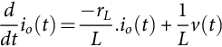
where rL and L are the resistance and inductance of the filter inductor, respectively, io(t) is the average inverter output current, and v(t) is the voltage, averaged in a switching period and applied to the inductor. The voltage on the inductor can be written as v(t)=vo(t)−vg(t), where vg(t) is the grid voltage and vo(t) is the averaged value of the inverter voltage.
The general solution of the differential equation is

where lower (t0) and upper (t) limits of integration can be defined as kTs and (k+1)Ts, respectively, to obtain discrete-time model with sampling period Ts.
where io(k)≡io(kTs). Ts is usually small enough to satisfy (rLTs/L) <<l; thus, (40.32) can be approximated as
Since d(t) is actualized every sampling period, we can assume that vo(t) is constant between two sampling instants:
if t ![]() [ kTs,(k+1)Ts]. On the other hand, as the sampling frequency is much higher than the grid frequency, we can approximate vg(t) linearly between two sampling instants:
[ kTs,(k+1)Ts]. On the other hand, as the sampling frequency is much higher than the grid frequency, we can approximate vg(t) linearly between two sampling instants:

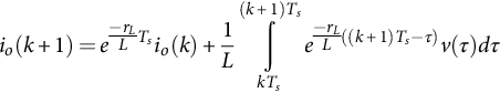
if t ϵ[kTs,(k+1)Ts]. Discrete-time model of the output current can be obtained from substituting (40.34) and (40.35) into (40.33):
where ![]() is the averaged value of the grid voltage between two samples.
is the averaged value of the grid voltage between two samples.
The cost function is an important stage of the MPC technique. To minimize the error between the reference and the predicted values in the next sampling time, the cost function must be selected according to specific design criteria. In this study, in order to control the output current, the cost function is defined as
where io*(k+1) is the reference output current and io(k+1) is the predicted output current in the next sampling time.
C. Implantation results
To verify the proposed MPC scheme for 33-level ISMI, experimental studies have been carried out for different operating conditions. The parameters of the system are summarized in Table 40.5.
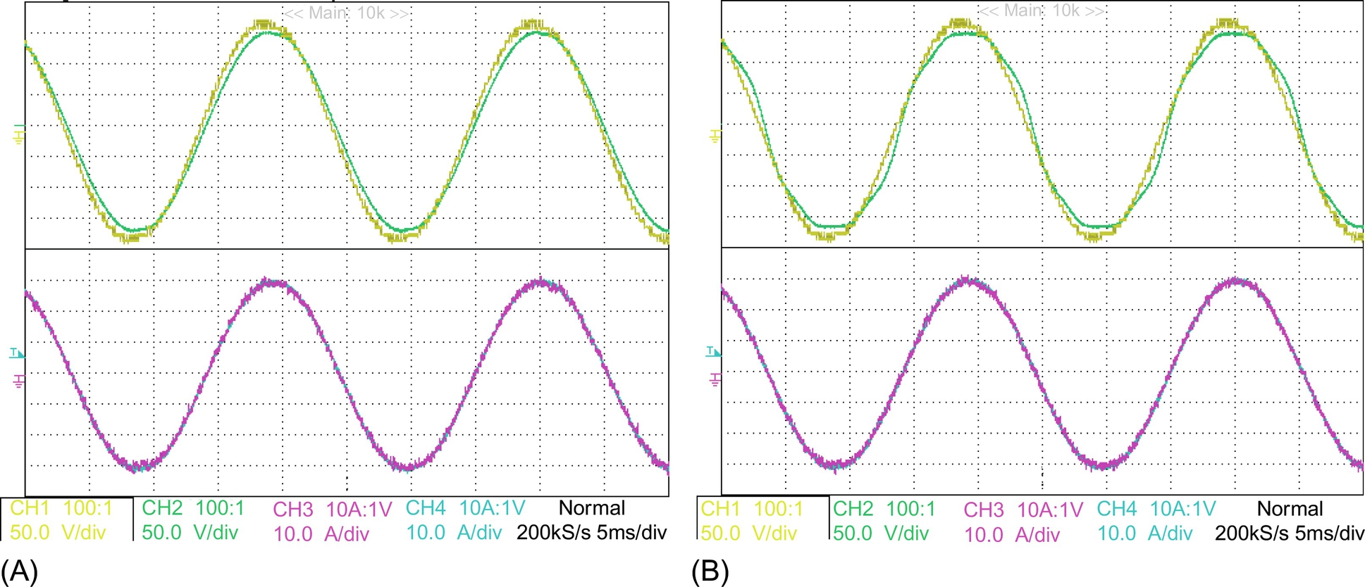
Fig. 40.17A and B shows the experimental results of steady-state performance of the MPC-based current controller under normal and poor grid conditions. The results show that even with poor grid condition, the MPC-based current controller has an excellent steady-state performance.
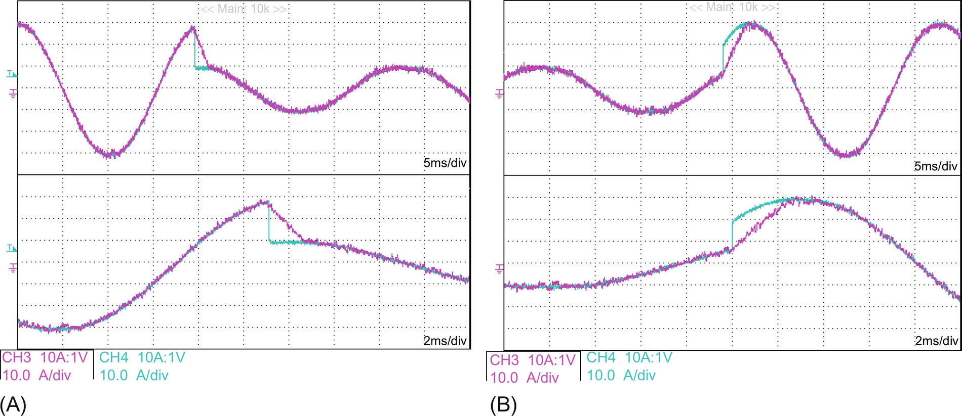
Fig. 40.18 shows the transient response results of the proposed MPC. The reference current is changed from 30 to 10 A and vice versa in order to observe the response of the proposed control technique. It can be seen that the transient time is very short, controller response is very fast, and the output current tracks its reference with high accuracy.
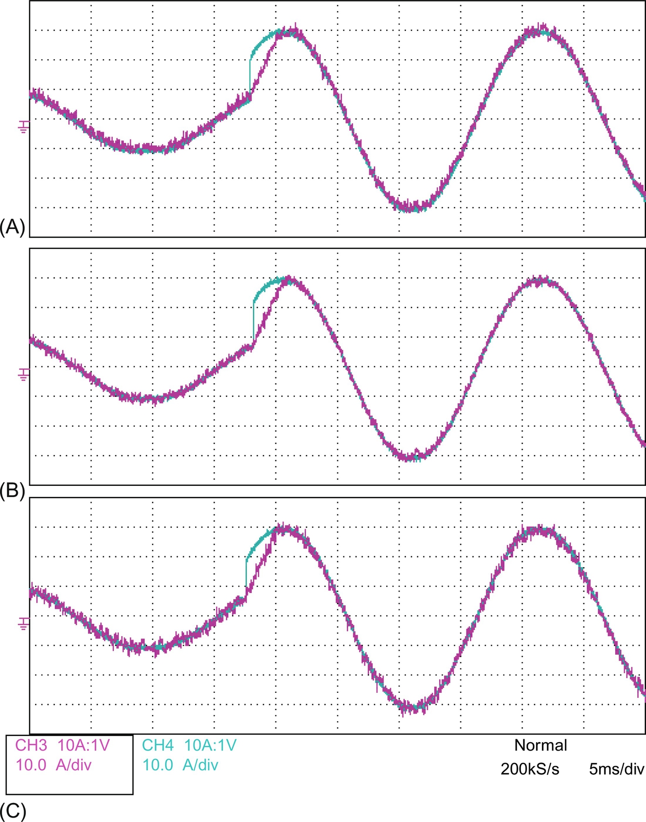
As the proposed control method is based on the system model, the algorithm is also tested to verify the robustness against the mismatch with filter parameter. To do that, the filter inductance (Lf) is consecutively set at 0.5*L, L, and 1.5⁎L, which is the typical case in distributed generation systems where the power system impedance changes randomly. It is remarkable that the new filter inductance value is not entered to the controller. The control algorithm uses a rated filter inductance value (L=10 mH). Results are shown in Fig. 40.19A–C. It is clear that, when the modeled inductance value is smaller than selected value (0.5*L), the mismatch causes steady-state errors, and when the modeled inductance value is bigger than selected value (1.5*L), the mismatch causes current oscillation. However, it can be observed from results that the mismatch of the filter model slightly affects the system performance.