
Novel AI-Based Soft Computing Applications in Motor Drives
Adel M. Sharaf University of Trinidad and Tobago UTT, Wallerfield, Trinidad and Tobago
Adel A.A. Elgammal University of Trinidad and Tobago UTT, Wallerfield, Trinidad and Tobago
Abstract
The chapter introduces novel ideas in the efficient control of industrial motor drives. The use of artificial intelligence (AI) soft computing techniques is gaining acceptance in the industry to ensure efficient energy utilization, robust and accurate speed reference tracking, minimum impact on the host electric grid system, and extended life span of the motor drive system while avoiding magnetic saturation and inrush current conditions. The use of emerging soft computing random search techniques such as particle swarm optimization (PSO) and genetic algorithm (GA) is also gaining acceptance as effective tools in dynamic on line tuning, self-regulating, and adjustment of controller to ensure that specific objective functions are optimized. The use of dynamic on line self-adjusting error-driven control strategies is promising effective, robust, and efficient control strategies for DC and AC motor drives. The use of new topologies, converter architecture, and switching strategies is greatly facilitated by multiloop regulation and dynamic absolute error minimization using PSO and GA search algorithms. In this chapter, a review of PSO and GA search methods is followed by single- and multiobjective optimization search algorithms and how both soft computing AI-based technique can be applied to optimal operation of induction motor drives, hybrid photovoltaic-fuel cell-diesel-battery electric vehicle drive system, and finally, the novel self-regulating green plug-energy management energy economizer schemes developed by the first author as a number of an extended family of modulated power filters, switched capacitor compensators, and dynamic electric energy management devices and system.
Keywords
Particle swarm optimization; Genetic algorithm; Power system; Motor drives
38.1 Introduction
Solving an optimization problem is one of the common scenarios that occur in most engineering applications. Classical optimization techniques such as linear programming (LP) and nonlinear programming (NLP) are efficient approaches that can be used to solve special cases of optimization problem in power system and motor drive applications. As the complexities of the problem increase, especially with the introduction of parameter uncertainties, more complicated optimization techniques, such as stochastic programming, have to be used. However, these analytic methods are not easy to implement for most of the real-world problems. As a highly nonlinear, nonstationary motor drive system with nonlinear inertia, load, noise, and uncertainties, motor drives can have a large number of operating condition states and parameters. Implementing any of the classical analytic optimization search methods may not be feasible in most of the cases. On the other hand, GA and particle swarm optimization (PSO) search techniques can be an attractive alternative and effective solutions. GA and PSO are stochastically based search techniques that have its roots in artificial life and social psychology and in engineering and computer science. In general, there are two possible optimization techniques based on GA and PSO. These two techniques are the following:
(1) Single-objective optimization (SOO)
(2) Multiobjective optimization (MOO)
The main procedure of the SOO is based on deriving a single-objective function for the optimization search problem. The single-objective function may be combined from several objective functions using weighting factors. The objective function is optimized (either minimized or maximized) using GA or PSO to obtain a single solution. On the other hand, the main objective of the multiobjective (MO) problem is finding the set of acceptable trade-off optimal solutions. This set of accepted solutions is called Pareto front. These acceptable solutions give more ability to the user to make an informed decision by seeing a wide range of solutions that are optimum from an “overall” standpoint. Single-objective (SO) optimization may ignore this trade-off viewpoint. This chapter has described the basic concepts of GA and PSO and presents a review of some of the applications of GA and PSO in motor drive-based optimization problems to give the reader some insights of how GA and PSO can serve as acceptable near-optimal solutions to some of the most complicated engineering optimization problems.
38.2 Differences Between GA and PSO and Other Evolutionary Computation Techniques
A comparison between conventional optimization techniques and evolutionary algorithms (like GA and PSO) is presented in Table 38.1 [1]:
Table 38.1
Comparison between conventional optimization procedures and evolutionary algorithms
| Property | Evolutionary | Traditional |
| Search space | Population of potential solutions | Trajectory by a single point |
| Motivation | Natural selection and social adaptation | Mathematical properties (gradient, Hessian) |
| Applicability | Domain independent, applicable to variety of problems | Applicable to a specific problem domain |
| Point transition | Probabilistic | Deterministic |
| Prerequisites | An objective function to be optimized | Auxiliary knowledge such as gradient vectors |
| Initial guess | Automatically generated by the algorithm | Provided by user |
| Flow of control | Mostly parallel | Mostly serial |
| CPU time | Large | Small |
| Results | Global optimum more probable | Local optimum, dependent of initial guess |
| Advantages | Global search, parallel, speed | Convergence proof |
| Drawbacks | No general formal convergence proof | Locality, computational cost |
➢ Unlike other random search algorithms, each potential solution (called a particle) is also assigned a randomized velocity and then flown through the problem hyperspace.
➢ The most striking difference between the PSO and the other evolutionary soft computing algorithms is that PSO chooses the path of cooperation over competition. The other algorithms commonly use some form of decimation, survival of the fittest. In contrast, the PSO population is stable and individuals are not destroyed or created. Individuals are influenced by the best performance of their neighbors. Individuals eventually converge on optimal points in the problem domain.
➢ The PSO traditionally does not have any genetic operators like crossover between individuals and mutation, and other individuals never substitute particles during the run. Instead, the PSO refines its search by attracting the particles to positions with good solutions.
➢ Particles update themselves with the internal velocity.
➢ They also have memory, which is important to the algorithm.
➢ Compared with GA, the information sharing mechanism in PSO is significantly different. In GAs, chromosomes share information with each other. So the whole population moves like one group toward an optimal area. In PSO, only gbest or pbest gives out the information to others. It is a one-way information sharing mechanism. The evolution only looks for the best solution.
➢ Compared with the GA, the advantages of PSO are that PSO is easy to implement and there are few parameters to adjust.
38.3 Single Objective Genetic Optimization Search Algorithm (SOGA)
GAs are an evolutionary optimization approach that is an alternative to traditional optimization methods. GA is most appropriate for complex nonlinear models where location of the global optimum is a difficult task. It may be possible to use GA techniques to consider problems that may not be modeled as accurately using other approaches.
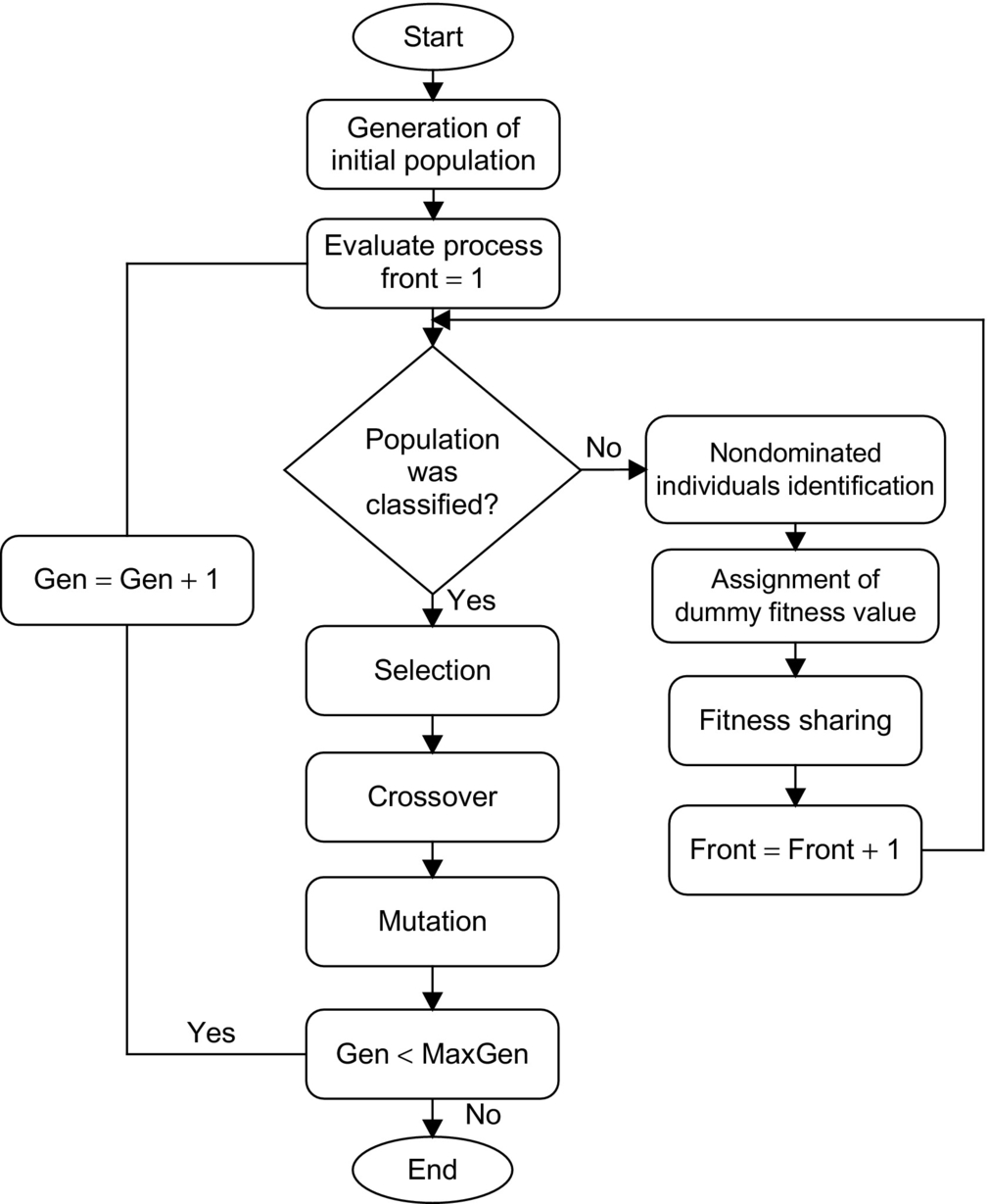
Therefore, GA appears to be a potentially useful approach. GA is particularly applicable to problems that are large, nonlinear, and possibly discrete in nature, features that traditionally add to the degree of complexity of solution. Due to the probabilistic development of the solution, GA does not guarantee optimality even when it may be reached. However, they are likely to be close to the global optimum. This probabilistic nature of the solution is also the reason they are not contained by local optima. The GA procedure is based on the Darwinian principle of survival of the fittest. An initial population is created containing a predefined number of individuals (or solutions), each represented by a genetic string (incorporating the variable information). Each individual has an associated fitness measure, typically representing an objective value. The concept that fittest (or best) individuals in a population will produce fitter offspring is then implemented in order to reproduce the next population. Selected individuals are chosen for reproduction (or crossover) at each generation, with an appropriate mutation factor to randomly modify the genes of an individual, in order to develop the new population. The result is another set of individuals based on the original subjects leading to subsequent populations with better (min or max) individual fitness. Therefore, the algorithm identifies the individuals with the optimizing fitness values, and those with lower fitness will naturally get discarded from the population [2]. Fig. 38.1 shows the general flowchart of the GA algorithm based on total error iterative minimum search. The steps of the GA are depicted as follows:
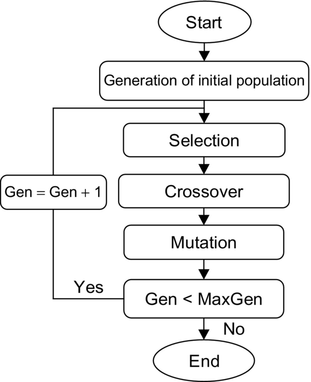
1. [Start] Generate random population of n chromosomes (suitable solutions for the problem).
2. [Fitness] Evaluate the fitness f(x) of each chromosome x in the population.
3. [New population] Create a new population by repeating following steps until the new population is complete:
a. [Selection] Select two parent chromosomes from a population according to their fitness (the better fitness, the bigger chance to be selected).
b. [Crossover] With a crossover probability cross over the parents to form a new offspring (children). If no crossover was performed, offspring is an exact copy of parents.
c. [Mutation] With a mutation probability, mutate new offspring at each locus (position in chromosome).
d. [Accepting] Place new offspring in a new population.
4. [Replace] Use new generated population for a further run of algorithm.
5. [Test] If the end condition is satisfied, stop, and return the best solution in current population.
[Loop] Go to step 2.
GAs can be applied to many scientific, engineering problems, once solutions of a given problem can be encoded to chromosomes in GA and compare the relative performance (fitness) of solutions. An effective GA representation and meaningful fitness evaluation are the keys of the success in GA applications. The appeal of GAs comes from their simplicity and elegance as robust search algorithms and from their power to discover good solutions rapidly for difficult high-dimensional problems. The main advantage of GA is that models that cannot be developed using other solution methods without some form of approximation can be considered in an unapproximated form. The size of the model, that is, number of probabilistic variables, has a significant effect on the speed of solution; therefore, model specification can be crucial. Unlike other solution methods, integer variables are easier to accommodate in GA than continuous variables. This is due to the resulting restricted search space. Further, variable bound values can be applied to achieve similar results. GAs can be used for problem-solving and for modeling when the search space is large, complex, or poorly understood. Domain knowledge is scarce or expert knowledge is difficult to encode to narrow the search space. No mathematical analysis is available and traditional search methods fail.
38.4 Single Objective Particle Swarm Optimization Search Algorithm (SOPSO)
Particle swarm optimization (PSO) is an evolutionary computational technique (a search method based on a natural system), which was introduced by Kennedy and Eberhart in 1995 [3]. This optimization and search technique models the natural swarm behavior seen in many species of birds returning to roost, group of fish, and swarm of bees, etc. The particle swarm optimization (PSO) may be used to find optimal (or near-optimal) solutions to numerical and qualitative problems [4–8]. PSO methods are inspired by particles moving around in the defined search space. The individuals in a PSO have a position and a velocity. The PSO method remembers the best position found by any particle. Additionally, each particle remembers its own previously best-found position. A particle moves through the specified solution space along a trajectory defined by its velocity, the draw to return to a previous promising search area, and an attraction toward the best location discovered by its close neighbors. Particle swarm optimization has been used for a wide range of search applications and for specific optimization tasks. PSO can be easily implemented in most programming languages and has proved to be both effective and fast when applied to a diverse set of nonlinear optimization problems. PSO has been successfully applied in many areas:
• Artificial neural network training
• Proportional and integral fuzzy system control
• Other near-optimal search and optimization areas where GA can be applied
38.4.1 Structure of the PSO Particle
The basic structure of any particle in a selected population consists of five components:
• →x![]() is a vector containing the current location in the solution space. The size of →x
is a vector containing the current location in the solution space. The size of →x![]() is defined by the number of variables used by the problem that is being solved.
is defined by the number of variables used by the problem that is being solved.
• Fitness is the quality of the solution represented by the vector →x![]() , as computed by a problem-specific evaluation function.
, as computed by a problem-specific evaluation function.
• →V![]() is a vector containing the velocity for each dimension of →x
is a vector containing the velocity for each dimension of →x![]() . The velocity of a dimension is the step size that the corresponding →x
. The velocity of a dimension is the step size that the corresponding →x![]() value will change into at the next iteration. Changing the →V
value will change into at the next iteration. Changing the →V![]() values changes the direction the particle will move through in the search space, causing the particle to make a turn. The velocity vector is used to control the range and resolution of the search.
values changes the direction the particle will move through in the search space, causing the particle to make a turn. The velocity vector is used to control the range and resolution of the search.
• Pbest is the fitness value of the best solution yet found by a particular particle.
• →P![]() is the copy of the →x
is the copy of the →x![]() for the location that generated the particle's Pbest. Jointly, Pbest and →x
for the location that generated the particle's Pbest. Jointly, Pbest and →x![]() comprise the particle's memory, which is used to control the particle to go back toward a definite search region.
comprise the particle's memory, which is used to control the particle to go back toward a definite search region.
• Each particle is also aware of the current best fitness in the neighborhood for any given iteration. A neighborhood may consist of some small group of particles, in which case the neighborhoods overlap and every particle is in multiple neighborhoods. Particles in a swarm are related socially; that is, each particle is a member of one or more neighborhoods. Each individual tries to emulate the behavior of the best of its neighbors. Each individual can be thought of as moving through the feature space with a velocity vector that is influenced by its neighbors.
38.4.2 Basic Search Method
The position of each particle is represented by XY-axis position, and also, the velocity is expressed by Vx (the velocity of X-axis) and Vy (the velocity of Y-axis). Modification of the particle position is realized by the position and velocity information. Each particle knows its best value so far (Pbest) and its XY position. This information represents the personal experiences of each particle. Moreover, each particle knows the best value so far in the group (gbest) among Pbests. This information represents the knowledge of how the other particles around have performed. Namely, each particle tries to modify its position using the following information:
• The current positions (x, y)
• The current velocities (Vx, Vy)
• The distance between the current position and Pbest
• The distance between the current position and gbest
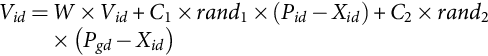
This modification can be represented by the concept of velocity. Velocity of each particle can be modified by the following equation:
Vid=W×Vid+C1×rand1×(Pid−Xid)+C2×rand2×(Pgd−Xid)
where
• Vid is the value of dimension d in the velocity vector →v![]() for particle i.
for particle i.
• C1 is the cognitive learning selected rate.
• C2 is the social learning selected rate.
• rand1 and rand2 are random values on the range [0.1].
• Xid is the current position of particle i along dimension d.
• W is the selected weighting factor.
• Pid is the location along dimension d at which the particle previously had the best fitness measure.
• Pgd is the current location along dimension d of the neighborhood particle with the best fitness.
The basic concept of the PSO technique lies in accelerating each particle toward its Pbest and gbest locations, with a random weighted acceleration at each step, and this is illustrated in Fig. 38.2.
where
PK is the current position of a particle.
PK+1 is its modified position.
VK is its initial velocity.
VK+1 is its modified velocity.
Vpbest![]() is the velocity considering its pbest location.
is the velocity considering its pbest location.
Vgbest![]() is the velocity considering its gbest location.
is the velocity considering its gbest location.
Using the above concept, a certain velocity, which gradually gets close to Pbest and gbest, can be calculated. The current position (searching point in the solution space) can be modified by the following equation:
Xid=Xid+Vid
38.4.3 PSO Search Algorithm
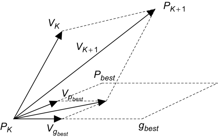
Fig. 38.3 shows the general flowchart of the PSO algorithm. The main steps in the particle swarm optimization process are described as follows:
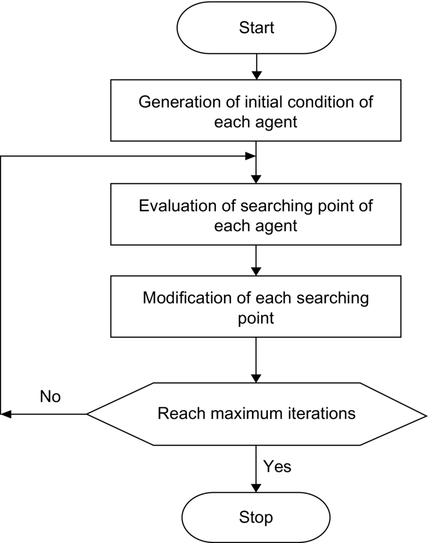
1. System initialized with a population of random potential solutions. Each potential solution is assigned a random “velocity” and is called a particle. (It has position in the space, i.e., it is a point in the solution space and it has velocity.) These particles are then “flown” through the search space of potential solutions.
2. Evaluate the fitness of each particle in the swarm.
3. For every iteration, compare each particle's fitness with its previous best fitness (Pbest) obtained. If the current value is better than Pbest, then set Pbest equal to the current value and the Pbest location equal to the current location in the d-dimensional space.
4. Compare Pbest of particles with each other and update the swarm global best location with the greatest fitness (gbest).
5. The velocity of each particle is changed (accelerated) toward its Pbest and gbest. This acceleration is weighted by a random term. A new position in the solution space is calculated for each particle by adding the new velocity value to each component of the particle's position vector.
6. Repeat steps (2)–(5) until convergence is reached based on some desired single- or multiple-objective criteria.
38.5 Multiobjective Optimization (MOO)
In many real-life applications, multiple and often conflicting objectives need to be satisfied. Satisfying these conflicting objective functions is called multiobjective optimization (MO). For example, to place more functional blocks on a chip while minimizing that chip's area and/or power dissipation is a conflicting objective that needs performing a trade-off analysis [9,10]. The objective of MO optimization is to find a set of acceptable solutions and present them to the user, who will then choose from them. Generally, there are two general approaches to solve multiobjective optimization. The first approach lies in combining the individual objective functions into a single composite function. Determination of a single objective is possible with methods, such as the weighted sum method, but the problem lies in the correct selection of the weights. In practice, it can be very difficult to accurately select these weights, even for someone very familiar with the problem domain. In addition, optimizing a particular solution with respect to a single objective can result in unacceptable results with respect to the other objectives [11,12]. The second general approach is to obtain the optimal solution. There will be a set of optimal trade-offs between the conflicting objectives, but this optimal solution is called Pareto-optimal solution set or Pareto front [13,14]. A Pareto-optimal set is a set of solutions that are nondominated with respect to one another. While moving from one Pareto solution to another, there is always a certain amount of importance in one objective to achieve a certain amount of gain in the other. Generating the Pareto set has several advantages. The Pareto set allows the user to make an informed decision by seeing a wide range of options. The Pareto set contains the solutions that are optimum from an “overall” standpoint. SO optimization may ignore this trade-off viewpoint. This feature is useful since it provides better understanding of this system in which all the consequences of a decision with respect to all the objectives can be explored [9].
The following definitions are used in the proposed multiobjective optimization (MO) search algorithm:
Definition 1
The general MO problem requiring the optimization of N objectives may be formulated as follows:
Minimize
→y=→F(→x)=[→f1(→x),→f2(→x),→f3(→x),…,→fN(→x)]T
subjecttogj(→x)≤0j=1,2,…,M
where
→x⁎=[→x⁎1,→x⁎2,…,→x⁎P]T∈Ω
→y![]() is the objective vector, the →gi(→x)
is the objective vector, the →gi(→x)![]() represent the constraints, and→x⁎
represent the constraints, and→x⁎![]() is a P-dimensional vector representing the decision variables within a parameter space Ω. The space spanned by the objective vectors is called the objective space. The subspace of the objective vectors satisfying the constraints is called the feasible space.
is a P-dimensional vector representing the decision variables within a parameter space Ω. The space spanned by the objective vectors is called the objective space. The subspace of the objective vectors satisfying the constraints is called the feasible space.
Definition 2
A decision vector →x1∈Ω![]() is said to dominate the decision vector →x2∈Ω
is said to dominate the decision vector →x2∈Ω![]() (denoted by →x1≺→x1
(denoted by →x1≺→x1![]() ), if the decision vector →x1
), if the decision vector →x1![]() is not worse than →x2
is not worse than →x2![]() in all objectives and strictly better than →x2
in all objectives and strictly better than →x2![]() in at least one objective.
in at least one objective.
Definition 3
A decision vector →x1∈Ω![]() is called Pareto-optimal, if there does not exist another →x2∈Ω
is called Pareto-optimal, if there does not exist another →x2∈Ω![]() that dominates it. An objective vector is called Pareto-optimal, if the corresponding decision vector is Pareto-optimal.
that dominates it. An objective vector is called Pareto-optimal, if the corresponding decision vector is Pareto-optimal.
38.6 Multiobjective Genetic Optimization Search Algorithm (MOGA)
The nondominated sorting genetic algorithm (NSGA) is a multiobjective GA that was developed by Deb et al. [15]. This algorithm has been chosen over a conventional GA for three principal reasons: (a) no need to specify a sharing parameter, (b) a strong tendency to find a diverse set of solutions along the Pareto-optimal front, and (c) the ability to specify multiple objectives without the need to combine them using a weighted sum. The basic idea behind NSGA is the ranking process executed before the selection operation, as shown in Fig. 38.4. This process identifies nondominated solutions in the population, at each generation, to form nondominated fronts [16]; after this, the selection, crossover, and mutation usual operators are performed. In the ranking procedure, the nondominated individuals in the current population are first identified. Then, these individuals are assumed to constitute the first nondominated front with a large dummy fitness value [16]. The same fitness value is assigned to all of them. In order to maintain diversity in the population, a sharing method is then applied. Afterward, the individuals of the first front are ignored temporarily, and the rest of population is processed in the same way to identify individuals for the second nondominated front. A dummy fitness value that is kept smaller than the minimum shared dummy fitness of the previous front is assigned to all individuals belonging to the new front. This process continues until the whole population is classified into nondominated fronts. Since the nondominated fronts are defined, the population is then reproduced according to the dummy fitness values.
38.7 Multiobjective Particle Swarm Optimization Search Algorithm (MOPSO)
In MOPSO [9–14], a set of particles are initialized in the decision space at random. For each particle i, a position xi in the decision space and a velocity vi are assigned. The particles change their positions and move toward the so-far best-found solutions. The nondominated solutions from the last generations are kept in the archive. The archive is an external population, in which the so-far found nondominated solutions are kept. Moving toward the optima (maximum or minimum) is done in the calculations of the velocities as follows:
Vid=ω×Vid+C1×rand1×(Ppd−Xid)+C2×rand2×(Prd−Xid)
Xid=Xid+Vid
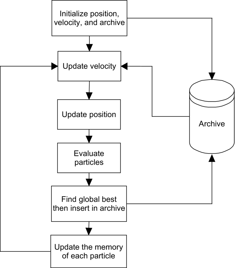
where Pr,d, Pp,d are randomly chosen from a single global Pareto archive, ω is the inertia factor influencing the local and global abilities of the algorithm, Vi,d is the velocity of the particle i in the d-th dimension, and c1 and c2 are weights affecting the cognitive and social factors, respectively. r1 and r2 are two uniform random functions in the range [0, 1]. According to Eq. (38.7), each particle has to change its position Xi,d toward the position of the two guides Pr,d, Pp,d that must be selected from the updated set of nondominated solutions stored in the archive. The particles change their positions during generations until a termination criterion is met. Finding a relatively large set of Pareto-optimal trade-off solutions is possible by running the MOPSO for many generations. Fig. 38.5 shows the flowchart of the multiobjective particle swarm optimization (MOPSO). Also, Fig. 38.6 explains the procedure of the multiobjective particle swarm optimization (MOPSO) using pseudocode.
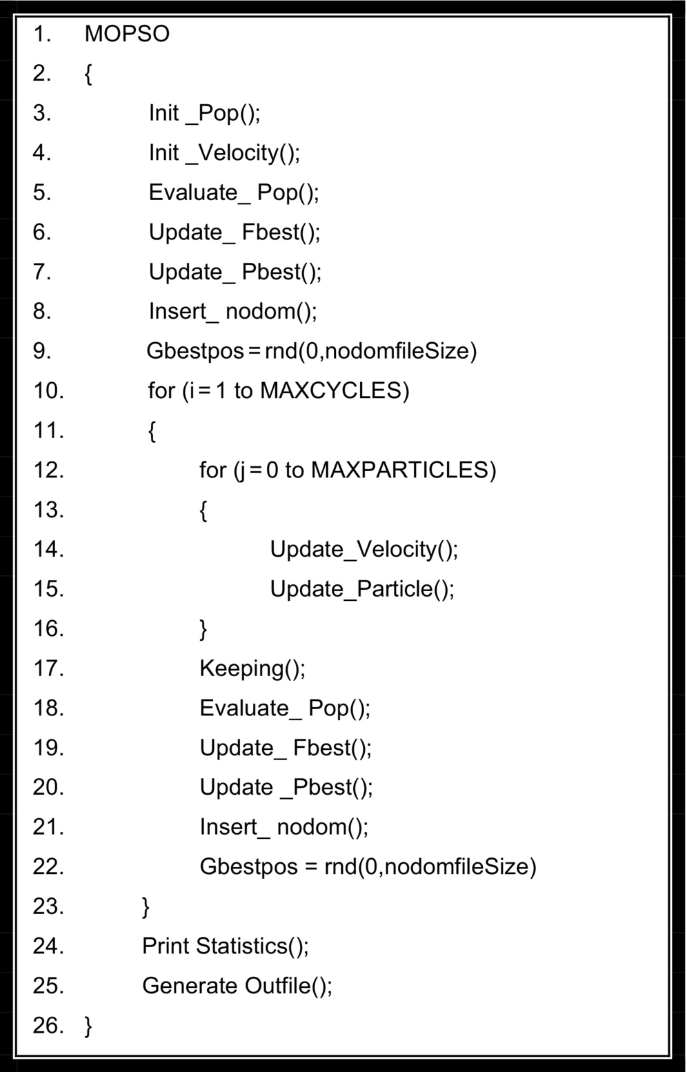
Init Pop(); The particle swarm is initialized with random values corresponding to the ranges of the decision variables. These values are dependent on the test functions.
Init Velocity(); The velocities are initialized with zero values.
Check the feasibility of each particle. If the particle does not satisfy the constraints, then regenerate it.
Evaluate Pop(); The swarm is evaluated using the corresponding objective functions.
Update Fbest(); The fitness vectors are updated (evaluate the multiobjective fitness value of each particle and save it in vector form). As we are dealing with multiobjective optimization, these vectors store the values of each decision variable, whereby the particles obtain the best values in a Pareto sense.
At this stage of the algorithm, these vectors are filled with the results of the initial particle evaluations.
Update Pbest(); Analogously, these values are copied in the pbest vectors.
Insert nodom(); Calculate the multiobjective fitness values of each particle and check its Pareto optimality. Store the nondominated particles in the Pareto archive. If the specific constraint does not exist for the archive, the size of the archive will be unlimited (all nondominated particles are inserted in the grid, i.e., in the external file).
Gbestpos=rnd (0,nodomfileSize); The global gbest particle is randomly selected.
//The flight cycle starts here //
Update Velocity(); The velocity of each particle is updated, using Eq. (38.6). Two Pareto solutions are chosen randomly for Pr,d, Pi,d from the Pareto archive.
Update Particle(); The position of each particle is also updated using Eq. (38.7).
Keeping(); The keeping operation is carried out to maintain the particles into the allowable range values. Then, the particles are mutated. If the particle does not remain within the feasible solution region, it is discarded and mutated again.
Evaluate Pop(); Update Fbest(); Update Pbest();
The particles are evaluated; the fitness and pbest vector are, if appropriate, updated.
Insert nodom(); As the particles move in the search space because they have changed positions, the dominance of each particle is verified, and, if appropriate, they are inserted in the grid.
(a) Check the Pareto optimality of each particle. If the fitness value of the particle is nondominated when compared with the Pareto-optimal set in the archive, save it into the Pareto archive.
(b) In the Pareto archive, if a particle is dominated by a new one, then discard it.
Gbestpos=rnd(0,nodomfileSize); Then, the new gbest is randomly selected. Two Pareto solutions are chosen randomly for pp;d and pr;d from the Pareto archive.
Repeat the cycle until the number of generations reaches a given n.
// the end of the cycles //
Print Statistics(); Generate Outfile(); Print the statistics and generate an output file, which contains the nondominated particles.
38.8 GA and PSO Applications in Speed Control of Motor Drives
Many areas in power systems require solving one or more nonlinear optimization problems. While analytic methods might suffer from slow convergence and the problem of dimensionality, GA and PSO are known to effectively solve large-scale nonlinear optimization problems [17]. This section provides some motor drives applications that have benefited from the powerful nature of GA and PSO as an optimization techniques. For each application, technical details that are required for applying GA and PSO and the most efficient fitness functions are also discussed. In this section, online energy optimization controllers are proposed for induction motor drives and PMDC motor drives using GA and PSO. In many applications, efficiency optimization of induction motors and PMDC motors represents an important factor of control especially for autonomous electric traction. This section will present some of the applications of GA and PSO in motor drive-based optimization problems to give some insight of how GA and PSO can serve as a solution to some of the most complicated engineering optimization problems [18–43].
38.8.1 Efficient Operation of Induction Motor Drives [18]
Induction motor is a high-efficiency electrical machine when working close to its rated torque and speed. However, at light loads, no balance in between copper and iron losses results considerable reduction in the efficiency. The part load efficiency and power factor can be improved by making the motor excitation adjustment in accordance with load and speed. To implement the above goal, the induction motor should either be fed through an inverter or redesigned with optimization algorithms [19]. This application presents an optimization technique for an efficient controller for the three-phase induction motors. Multiobjective particle swarm optimization (MOPSO) technique is implemented to tackle all the conflicting goals that define the search for the optimality problem. The PSO search deals with two main conflicting objective functions. These conflicting functions are maximizing the operating efficiency of the drive system for a given mechanical load and maximizing the equivalent power factor of the induction motor for start-up and steady-state operations. In addition, the optimization ensures that maximum allowable stator current constraints are not exceeded. The proposed technique are based on the principle that the flux level in a machine can be adjusted to give the required trade-off solution of maximum efficiency and maximum power factor for a given value of speed and load torque. The optimum flux levels are function of the machine load and speed requirements. Simulation results show that considerable efficiency and power factor improvements are achieved using MOPSO when compared with the field-oriented control (FOC) and constant voltage-to-frequency ratio-based control (CVFRC).
For optimal operation, three key objective functions that can affect the motor operation had been chosen. These three objective functions are based on motor efficiency, motor power factor, and motor stator current:
2. Power factor (to maximize)
3. Stator current (to minimize)
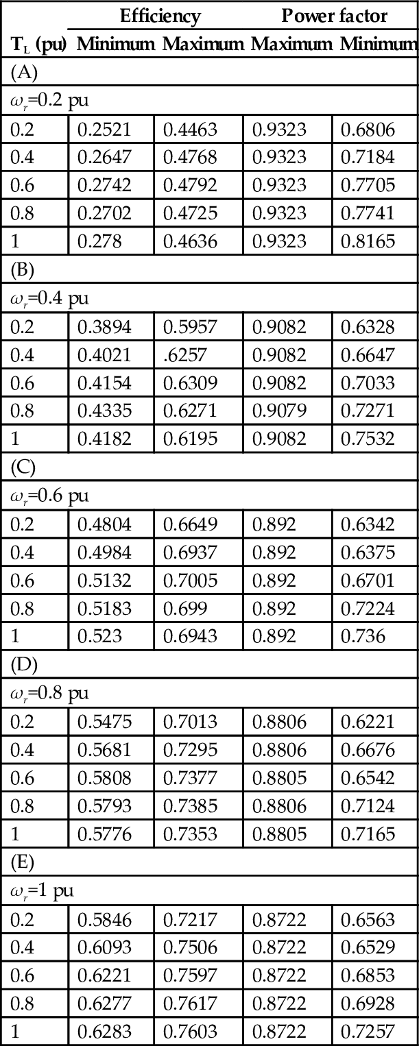
In addition, the optimization search ensures that all maximum stator current and inrush constraints are not exceeded. Fig. 38.7 is a plot of input power versus stator current. As illustrated in this figure, the stator current and the input power are minimized almost simultaneously. Therefore, in practice, the maximum efficiency (ME) and the minimum stator current (MSC) are not conflicting objective functions. So, when the efficiency is maximized, the stator current is minimized and the torque per ampere is maximized. So, the maximum efficiency and power factor will be considered as the main conflicting objective functions. However, a good operation should represent the right compromise among different objectives, but the problem consists in searching this “compromise.” The best tool to optimally solve this problem is represented by the multiobjective approach. This approach allows us to investigate how each single-objective and multiobjective problem affects the results in terms of performance and independent variables and, above all, allows us to have a wide range of alternative solutions among which the operator can choose a better solution. The MOGA and MOPSO algorithms have been applied to optimize the operation of a three-phase, 380 V, 1 hp, 50 Hz, four-pole, squirrel cage induction motor. The block diagram of the optimization process based on PSO is shown in Fig. 38.8. In the proposed controller, the PSO algorithm receives the rotor speed and load torque, and then, the PSO controller determines the slip frequency at which the optimal fitness function occurs at that rotor speed and load torque. As stated before, this part of simulation will consider the maximum efficiency and the maximum power factor (ME and MPF) problem to be solved using multiobjective particle swarm optimization. Fig. 38.9 shows the solution to this problem and shows the Pareto fronts of the problem for different levels of rotor speed ωr=0.2, 0.4, 0.8, 1 pu and different levels of load torque TL=0.2 and 1 pu. Tables 38.2 and 38.3 show the solution limits of the efficiency and the power factor for each operating point using MOGA and MOPSO. This range of solutions that is called the Pareto front enables the operator to choose the best compromise solution. Fig. 38.10 shows the comparison between the constant voltage-to-frequency ratio strategy (CVFRS), the field-oriented control strategy (FOCS), and the available solutions from MOPSO at different levels of load torque and rotor speed ωr=0.2 and 1 pu, respectively. The solution that has maximum efficiency is selected from the Pareto front to achieve this comparison. Keep in mind that the operator can choose the compromised solution from the Pareto front depending on the desired efficiency and power factor. It is obvious from Fig. 38.7 that the stator current is minimized using MOPSO. In addition, there is a great improvement in efficiency and power factor using MOPSO when compared with other strategies especially at light loads. It is noted that there is a very poor PF obtained using conventional methods (field-oriented control strategy and constant voltage-to-frequency ratio) especially at light loads. It is obvious from Fig. 38.9 that the efficiency improvement has a noticeable value especially at light loads and rotor speed ωr=0.2 pu that can be as high as 80% using CVFRS. This difference decreases to 65% at rotor speed ωr=1 pu. On the other hand, the power factor improvement reaches 55% at light load and rotor speed ωr=0.2 pu, whereas this improvement reaches to 160% at rotor speed ωr=1 pu and light load. The performance difference between the field-oriented control (FOC) and the proposed control strategies MOPSO comes from the chosen value of the slip frequency and the air gap flux for each strategy. For example, at loading condition of rotor speed equal to 0.2 pu and load torques varying from 0.2 to 1 pu, the values of slip frequency based on FOCS vary from 0.01 to 0.042 pu. On the other hand, the values of slip frequency based on MOPSO vary from0.0301 to 0.0524 PU. This difference in slip frequency and air gap flux causes the difference in performance of each control strategy. The difference in the flux level of the (FOCS) controller comes from the choice of the level of the magnetization current command. The command of magnetization current is set to a constant value, which produces rated torque at rated stator flux. At light loads, the constant chosen value of magnetization current fails to choose the optimal flux level. On the other hand, this value yields the optimal flux level at rated loads. The proposed strategies overcome this problem and successfully choosing the optimal flux level especially at light loads.
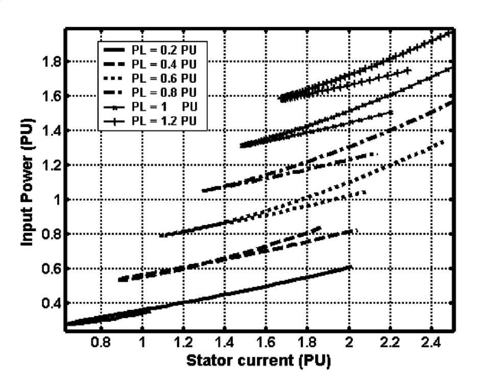
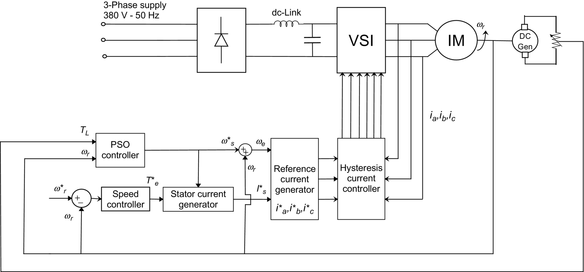
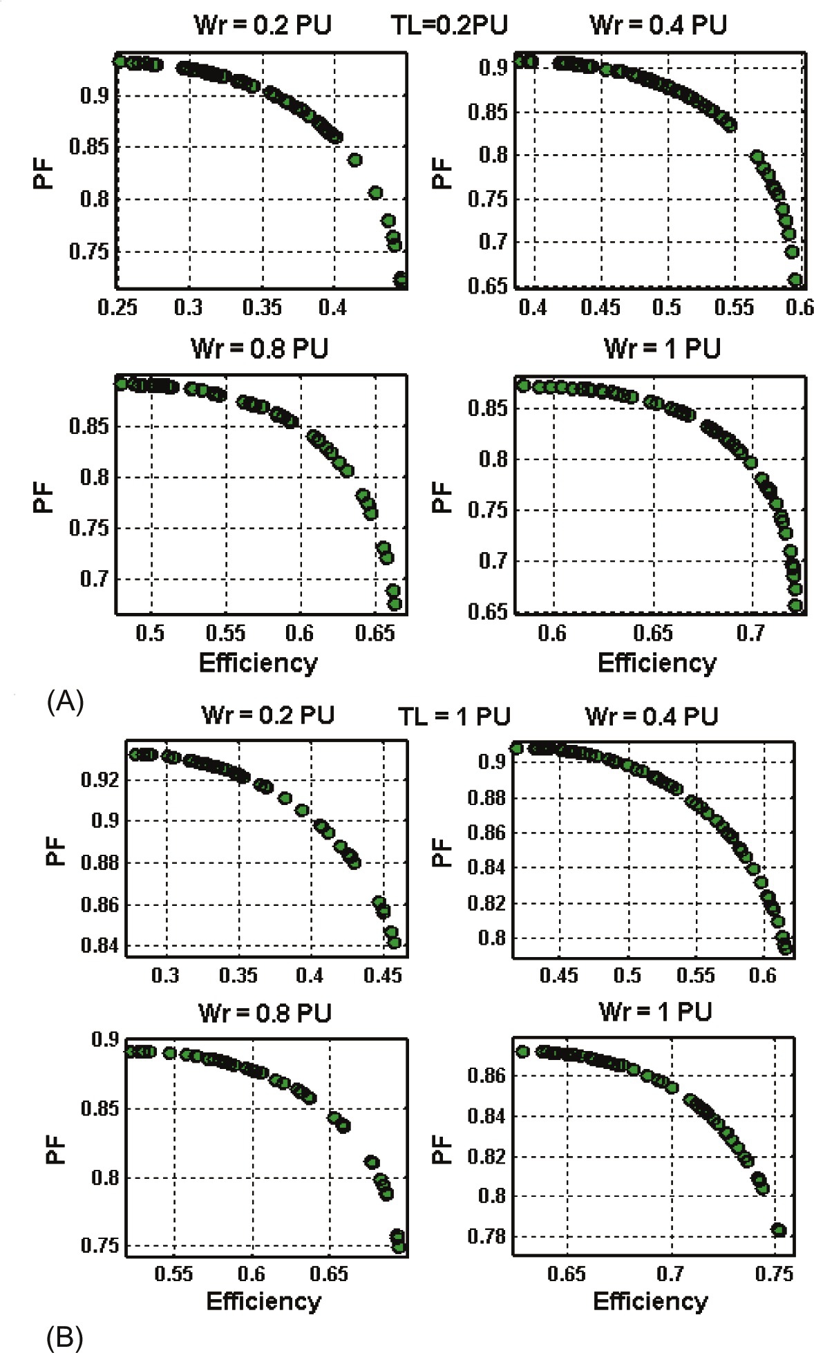
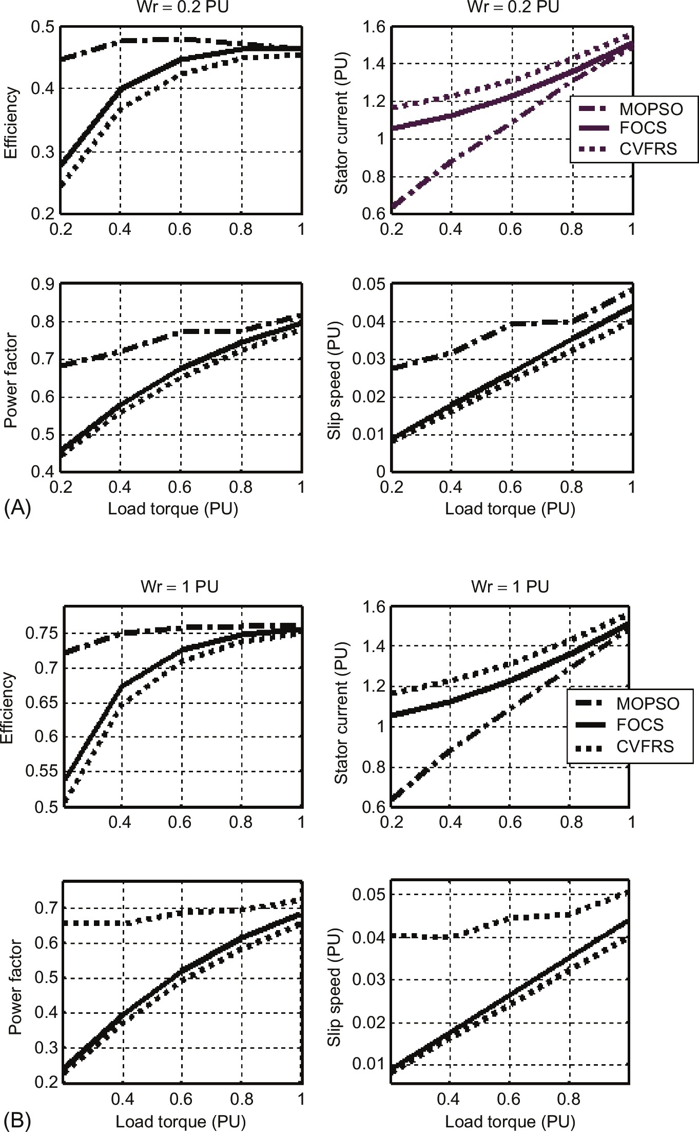
Table 38.2
The limits pf the Pareto front of the two conflicting objective functions using MOGA
| TL (pu) | Efficiency | Power factor | ||
| Minimum | Maximum | Maximum | Minimum | |
| (A) | ||||
| ωr=0.2 pu | ||||
| 0.2 | 0.2554 | 0.4665 | 0.9284 | 0.6650 |
| 0.4 | 0.2486 | 0.4544 | 0.9318 | 0.7091 |
| 0.6 | 0.2521 | 0.4371 | 0.9344 | 0.7780 |
| 0.8 | 0.2510 | 0.4688 | 0.9308 | 0.6578 |
| 1 | 0.2549 | 0.4539 | 0.9198 | 0.6771 |
| (B) | ||||
| ωr=0.4 pu | ||||
| 0.2 | 0.3571 | 0.5883 | 0.9010 | 0.6860 |
| 0.4 | 0.3934 | 0.6012 | 0.8862 | 0.7068 |
| 0.6 | 0.3784 | 0.5915 | 0.8963 | 0.6786 |
| 0.8 | 0.4025 | 0.5818 | 0.8871 | 0.6662 |
| 1 | 0.3794 | 0.5960 | 0.9008 | 0.6547 |
| (C) | ||||
| ωr=0.6 pu | ||||
| 0.2 | 0.4979 | 0.6859 | 0.8893 | 0.7015 |
| 0.4 | 0.4989 | 0.7099 | 0.8830 | 0.6641 |
| 0.6 | 0.5076 | 0.7053 | 0.8820 | 0.7114 |
| 0.8 | 0.5072 | 0.6948 | 0.8830 | 0.6872 |
| 1 | 0.4917 | 0.7051 | 0.8868 | 0.6695 |
| (D) | ||||
| ωr=0.8 pu | ||||
| 0.2 | 0.5301 | 0.7298 | 0.8753 | 0.6707 |
| 0.4 | 0.5270 | 0.7346 | 0.8744 | 0.6340 |
| 0.6 | 0.5251 | 0.7218 | 0.8738 | 0.6520 |
| 0.8 | 0.5299 | 0.7324 | 0.8722 | 0.6127 |
| 1 | 0.5285 | 0.7115 | 0.8781 | 0.7025 |
| (E) | ||||
| ωr=1 pu | ||||
| 0.2 | 0.5964 | 0.7170 | 0.8603 | 0.6899 |
| 0.4 | 0.5937 | 0.7337 | 0.8636 | 0.7032 |
| 0.6 | 0.5952 | 0.7423 | 0.8712 | 0.6599 |
| 0.8 | 0.5921 | 0.7314 | 0.8693 | 0.6919 |
| 1 | 0.5938 | 0.7366 | 0.8651 | 0.6593 |
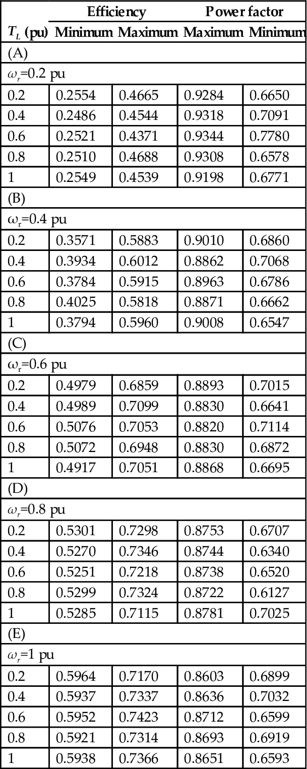
Table 38.3
The limits pf the Pareto front of the two conflicting objective functions using MOPSO
| TL (pu) | Efficiency | Power factor | ||
| Minimum | Maximum | Maximum | Minimum | |
| (A) | ||||
| ωr=0.2 pu | ||||
| 0.2 | 0.2521 | 0.4463 | 0.9323 | 0.6806 |
| 0.4 | 0.2647 | 0.4768 | 0.9323 | 0.7184 |
| 0.6 | 0.2742 | 0.4792 | 0.9323 | 0.7705 |
| 0.8 | 0.2702 | 0.4725 | 0.9323 | 0.7741 |
| 1 | 0.278 | 0.4636 | 0.9323 | 0.8165 |
| (B) | ||||
| ωr=0.4 pu | ||||
| 0.2 | 0.3894 | 0.5957 | 0.9082 | 0.6328 |
| 0.4 | 0.4021 | .6257 | 0.9082 | 0.6647 |
| 0.6 | 0.4154 | 0.6309 | 0.9082 | 0.7033 |
| 0.8 | 0.4335 | 0.6271 | 0.9079 | 0.7271 |
| 1 | 0.4182 | 0.6195 | 0.9082 | 0.7532 |
| (C) | ||||
| ωr=0.6 pu | ||||
| 0.2 | 0.4804 | 0.6649 | 0.892 | 0.6342 |
| 0.4 | 0.4984 | 0.6937 | 0.892 | 0.6375 |
| 0.6 | 0.5132 | 0.7005 | 0.892 | 0.6701 |
| 0.8 | 0.5183 | 0.699 | 0.892 | 0.7224 |
| 1 | 0.523 | 0.6943 | 0.892 | 0.736 |
| (D) | ||||
| ωr=0.8 pu | ||||
| 0.2 | 0.5475 | 0.7013 | 0.8806 | 0.6221 |
| 0.4 | 0.5681 | 0.7295 | 0.8806 | 0.6676 |
| 0.6 | 0.5808 | 0.7377 | 0.8805 | 0.6542 |
| 0.8 | 0.5793 | 0.7385 | 0.8806 | 0.7124 |
| 1 | 0.5776 | 0.7353 | 0.8805 | 0.7165 |
| (E) | ||||
| ωr=1 pu | ||||
| 0.2 | 0.5846 | 0.7217 | 0.8722 | 0.6563 |
| 0.4 | 0.6093 | 0.7506 | 0.8722 | 0.6529 |
| 0.6 | 0.6221 | 0.7597 | 0.8722 | 0.6853 |
| 0.8 | 0.6277 | 0.7617 | 0.8722 | 0.6928 |
| 1 | 0.6283 | 0.7603 | 0.8722 | 0.7257 |
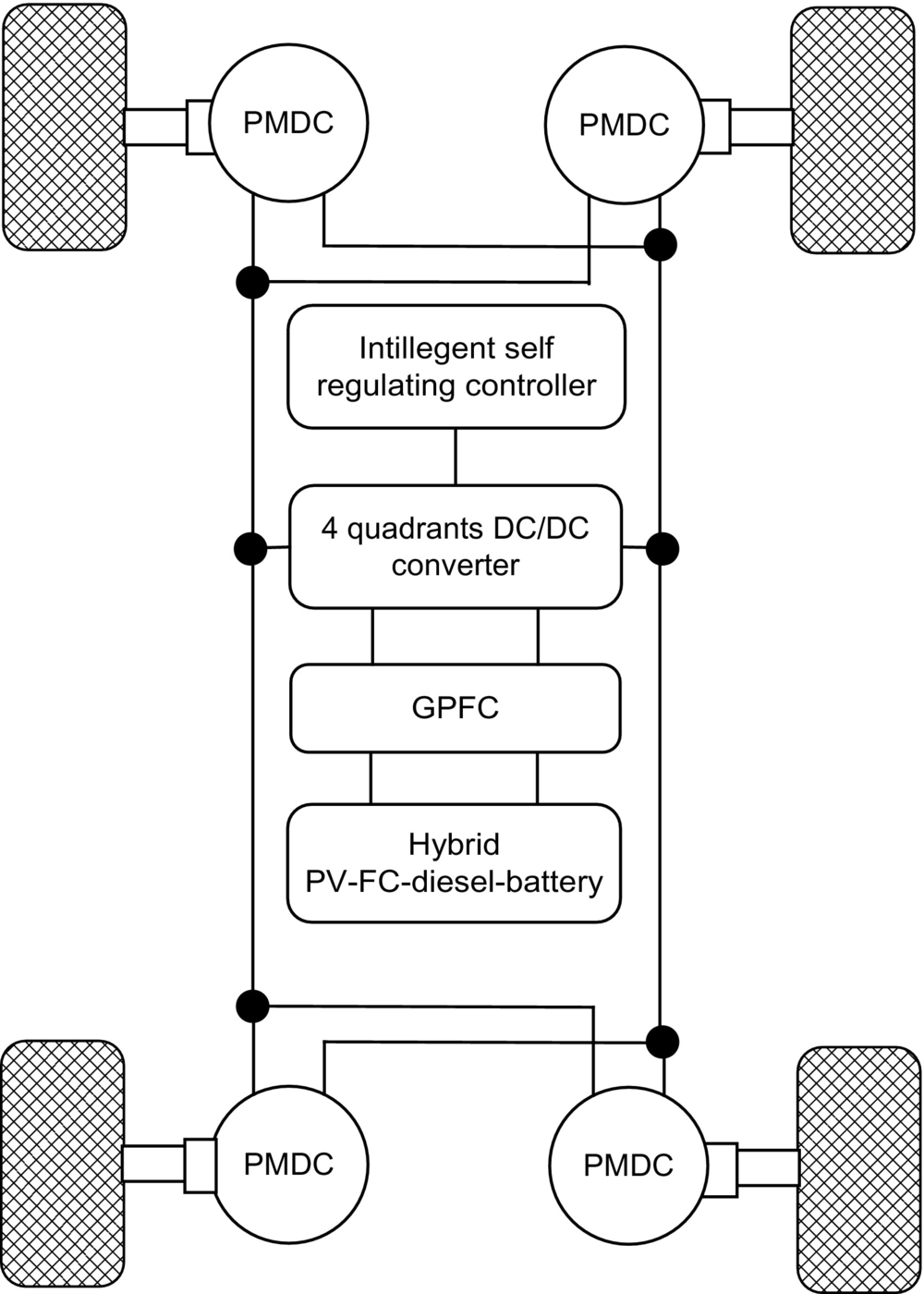
38.8.2 A Novel Self Regulating Hybrid (PV-FC-Diesel-Battery) Electric Vehicle-EV Drive System [20]
This application presents a number of novel self-regulating triloop error-driven controllers for a hybrid PV-FC-diesel-battery-powered all-wheel drive electric vehicle using four-wheel permanent magnet DC (PMDC) motors, which are modeled to include existing nonlinearities in motor plus load inertia (J) and viscous friction (B). A triloop dynamic error-driven scheme is proposed to regulate motor speed and current and avoid motor overloading/inrush conditions, in addition to motor speed dynamic reference tracking. The proposed triloop dynamic error-driven self-tuned control schemes are utilized to ensure dynamic energy efficiency, control loop decoupling, and grid interface stability while maintaining reference speed tracking capability. The integrated motor drive scheme is fully stabilized using novel FACTS-based green filter compensators that ensure stabilized DC bus voltage, minimal inrush current conditions, and damped load excursions. This application presents a novel comparison of multiobjective particle swarm optimization (MOPSO) and genetic search algorithms MOGA optimization and search techniques for online dynamic tuning of the different controllers under varying renewable source conditions and load excursions.
The pressing need to utilize all abundant renewable green energy sources (wind, solar, PV, wave, tidal, fuel cell, biogas, and hybrid) is currently motivated by economic and environmental concerns. The increasing reliance on costly fossil fuels with increasing rate of resource depletion is causing a shift to energy alternatives, clean fuel replacement, and energy displacement of conventional sources to new green renewable, environmentally safe, and friendly counterparts [21,22]. Electric vehicle is one of the solutions for the reduction of the fossil fuel consumption and pollutant emissions of gas, responsible for the greenhouse effect. However, pure battery electric vehicles have shown their own range limitations; because of their size, the vehicle habitability is reduced so as its range. Adding different kinds of power supply in the same vehicle allow taking advantages from their different characteristics [23]. Several types of electric motors may be used for EV propulsion purposes. Earlier traction motors were exclusively dc motors, either series excited or separately excited. Recently, more advanced ac drive systems have found application in EV propulsion using induction motors, permanent magnet synchronous motors, and permanent magnet brushless dc motors [24,25]. The EV-DC motor speed or position control has been realized including conventional PI, PID, fuzzy logic based, nonlinear, adaptive variable structure, model reference adaptive control, artificial neural networks, and feedforward computed torque control strategies [26–28]. The need for an online gains adaptation or a “tunable” control mechanism is highly stressed in the control of any nonlinear systems with unmodeled dynamics. The PSO- and GA-based self-regulating algorithms are utilized to track any reference speed trajectory under varying parameter and load conditions. The control system comprises four different controllers used to track speed reference trajectory depicting the motor with minimum overcurrent, inrush, and ripple conditions. The proposed novel control scheme has been validated for effective dynamic speed reference trajectory tracking and enhanced power utilization.
38.8.2.1 Sample Study AC-DC System
Figs. 38.11 and 38.12 show the proposed the four-wheel electric vehicle drive system scheme with the PV, FC sources, the diesel generator, and the backup battery. The DC compensator scheme developed by the first author is used to ensure stable, efficient, and minimal inrush operation of the hybrid renewable energy scheme. The novel PSO and GA self-tuned multiregulators and coordinated controller are used for the following purposes:
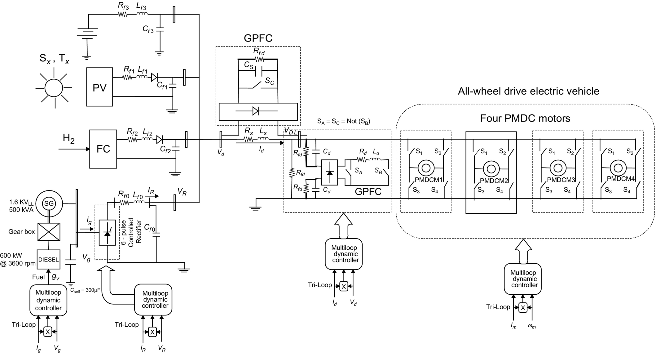
1. Diesel AC generator set with control regulator is based on excess generation and load dynamic matching and stabilization of the common DC collection bus using six-pulse-controlled rectifier.
2. AC/DC power converter regulator to regulate the DC voltage at the diesel engine AC/DC interface and ensure limited inrush conditions and dynamic power matching to reduce current transients and improve utilization at the diesel engine interface AC-DC bus.
3. The DC side green plug filter compensator GPFC-SPWM regulator for pulse-width switching scheme to regulate the DC bus voltage and minimize inrush current transients and load excursions and/or PV and FC nonlinear volt-ampere characteristics. The GPFC device acts as a matching DC-DC interface device between the DC load dynamic characteristics and that of the hybrid main PV, FC, and backup diesel generator set.
4. The permanent magnet DC motor drive with the speed regulator that ensures speed reference tracking with minimum inrush conditions and ensures reduced voltage transients and improved energy utilization.
The unified DC-AC utilization scheme is fully validated using the Matlab/Simulink software environment under normal conditions, DC load excursion, PMDC motor torque changes and the PV, and FC source output variations due to the inherent volt-ampere nonlinear relationship. Other excursion conditions in the diesel engine generator set are also introduced to assess the control system robustness, effective energy utilization, and speed reference tracking.
Diesel generator set
From an electric system point of view, a diesel-driven AC generator can be represented as a prime mover and generator. Ideally, the prime mover has the capability to supply any power demand up to rated power at constant synchronous frequency. The synchronous generator connected to it must be able to keep the voltage constant at any load condition. The diesel engine kept the operating speed and frequency constant. When power demand fluctuates, the diesel generator could vary its power output via fuel valve regulation and governor control. The synchronous generator must control its output voltage by controlling its excitation current. Thus, the diesel generating system, as an auxiliary source, must be able to control its frequency and its output voltage. The ability of the diesel generator to respond to any frequency changes is affected by the inertia of the diesel gen set, the sensitivity of the governor, and the power capability of the diesel engine. The ability of the AC synchronous generator to control its terminal voltage can be affected by the field-winding time constant, the availability of DC excitation power to supply the field winding, and the time constant of the voltage control loop.
Photo voltaic PV
The equivalent circuit shown in Fig. 38.13 is used to model the PV cells used in the proposed PV array [29]. This model consists of a current source, a resistor, and a reverse parallel connected diode. The PVA model developed and used in Matlab/Simulink environment is based upon the circuit given in Fig. 38.13, in which the current produced by the solar cell is equal to that produced by the current source, minus that which flows through the diode, minus that which flows through the shunt resistor:
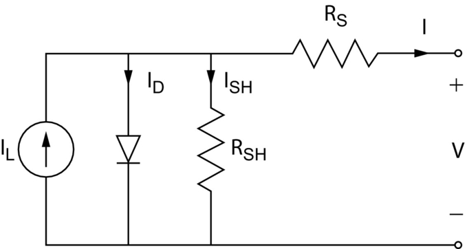
I=IL−ID−ISH
where I=output current, IL=photo-generated current, ID=diode current, and ISH=shunt current. The current through these elements is governed by the voltage across them:
Vj=V+IRS
where Vj=voltage across both diode and resistor RSH (volts), V=voltage across the output terminals (volts), I=output current (amperes), and RS=series resistance (Ω).
The current diverted through the diode is
ID=Io{exp[qVjnkT]−1}
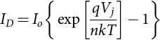
where I0=reverse saturation current (amperes), n=diode ideality factor (1 for an ideal diode), q=elementary charge, k=Boltzmann's constant, and T=absolute temperature.
The characteristic equation of a solar cell, which relates solar cell parameters to the output current and voltage [30]:
I=IL−Io{exp[q(V+IRs)nkT]−1}−V+IRsRSH
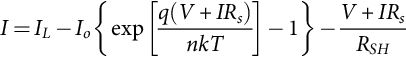
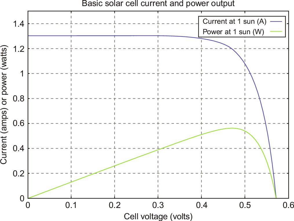
where RSH=shunt resistance (Ω). The I-V curve of an illuminated PV cell has the shape shown in Fig. 38.14 as the voltage across the measuring load is swept from zero to VOC, The power produced by the cell in watts can be easily calculated along the I-V sweep by the equation P=IV. At the ISC and VOC points, the power will be zero, and the maximum value for power will occur between the two.
Fuel cell energy system model
Fuel cell stacks were connected in series/parallel combination to achieve the rating desired. Fig. 38.15 shows a simplified diagram of the PEMFC system [31,32]. The FC model here is for a type of PEM, which uses the following electrochemical reaction:
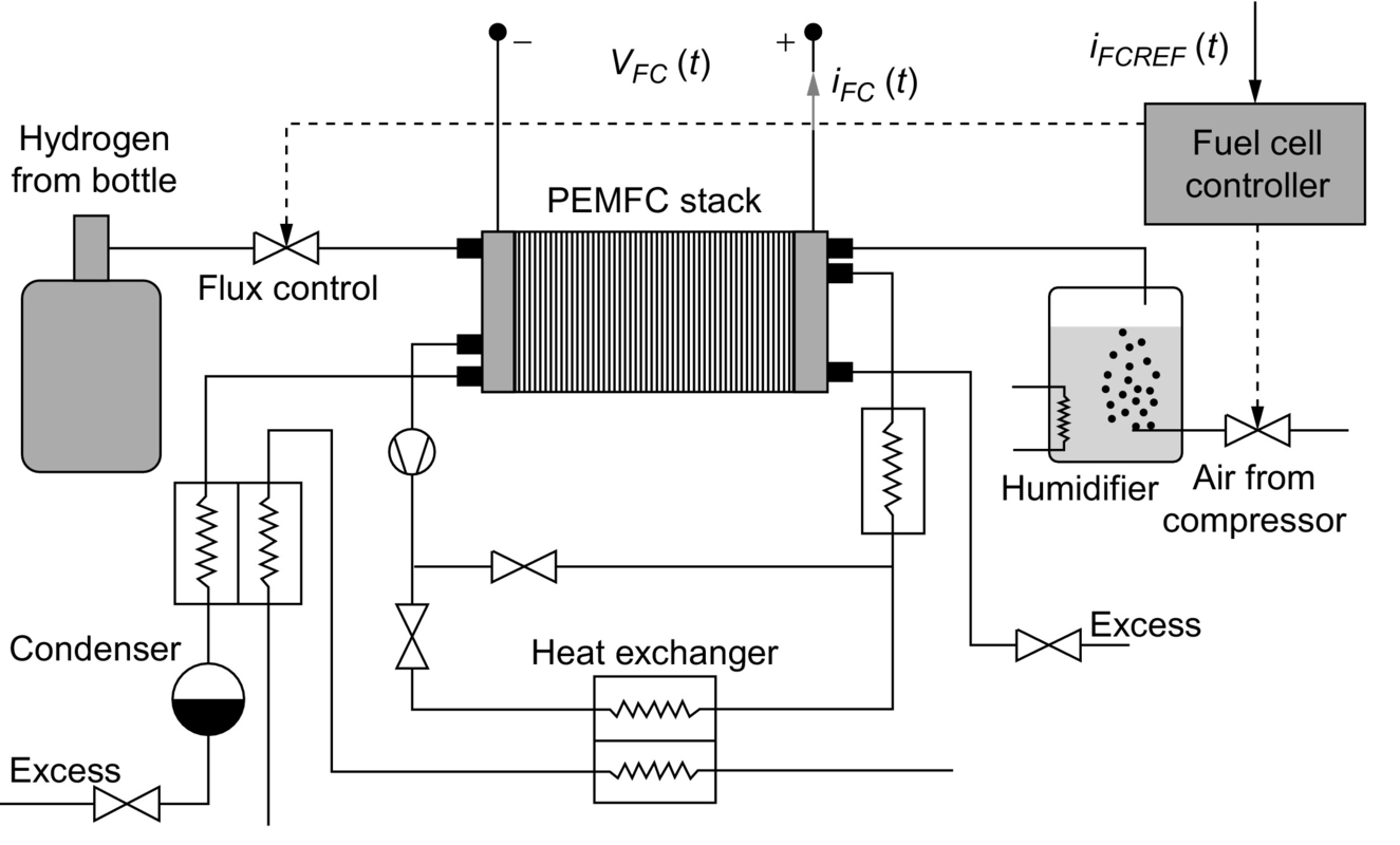
H2+12O2→H2O+Heat+ElectricalEnergy
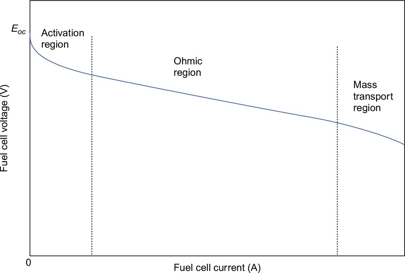
Fig. 38.16 shows a simulated V-I (voltage versus current) polarization curve of a fuel cell [31,32]. As the cell current begins to increase from zero, a sudden drop of the output voltage of the fuel cell is seen. This drop of the cell voltage is due to activation voltage loss. Then, almost a linear decrease of the cell voltage is seen as the cell current increases beyond certain values, as shown in Fig. 38.17, which is a result of the ohmic loss. Finally, the cell voltage drops sharply to zero as the load current approaches the maximum current density that can be generated of the fuel cell. The sharp voltage drop is the effect of the concentration loss in the fuel cell. The fuel cell can be commonly modeled by simple equivalent first-order circuit shown in Fig. 38.10. The open circuit voltage is modified as follows:
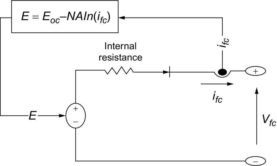
Eoc=N(En−Aln(io))
where
A=RTZαF

where R=8.3145 J/(mol K); F=96,485 As/mol; z=number of moving electrons; En=Nernst voltage, which is the thermodynamics voltage of the cells and depends on the temperatures and partial pressures of reactants and products inside the stack; and i0=exchange current, which is the current resulting from the continual backward and forward flow of electrons from and to the electrolyte at no load. It depends also on the temperatures and partial pressures of reactants inside the stack. α is the charge transfer coefficient, which depends on the type of electrodes and catalysts used and T is the temperature of operation. The fuel cell voltage VFC is modeled as [31,32]
VFC=Eoc−VActivationloss−VOhmicloss−VConcentrionloss
where
VActivationLoss=Alog(IFC+inio)
VOhmicLoss=Rm(IFC+in)
VConcentrationLoss=Blog(1−IFC+iniL)
Fuel cell stacks were connected in series/parallel combination to achieve the rating desired. The output of the fuel cell array was connected to a DC bus through a DC/DC converter. The DC bus voltage was kept constant via a DC bus voltage controller.
DC side green plug filter compensator GPFC
The common concerns of power quality are the long-duration voltage variations (overvoltage, undervoltage, and sustained interruptions), short-duration voltage variations (interruption, sags, and swells), voltage imbalance (voltage unbalance), waveform distortion (DC offset, harmonics, interharmonics, notching, and noise), voltage fluctuation (voltage flicker), and power frequency variations [33]. To prevent the undesirable states and to reduce the power consumption, a GPF scheme is used to stabilize the common DC bus.
Dynamic error driven control
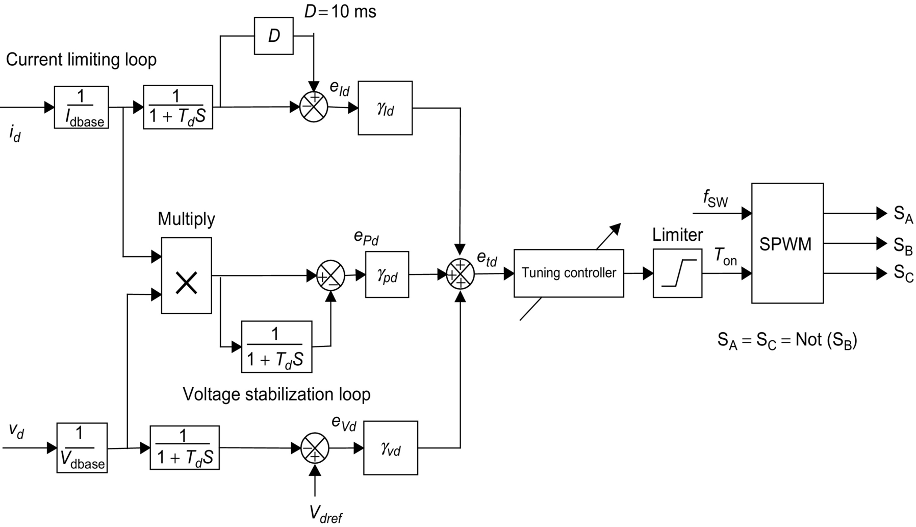
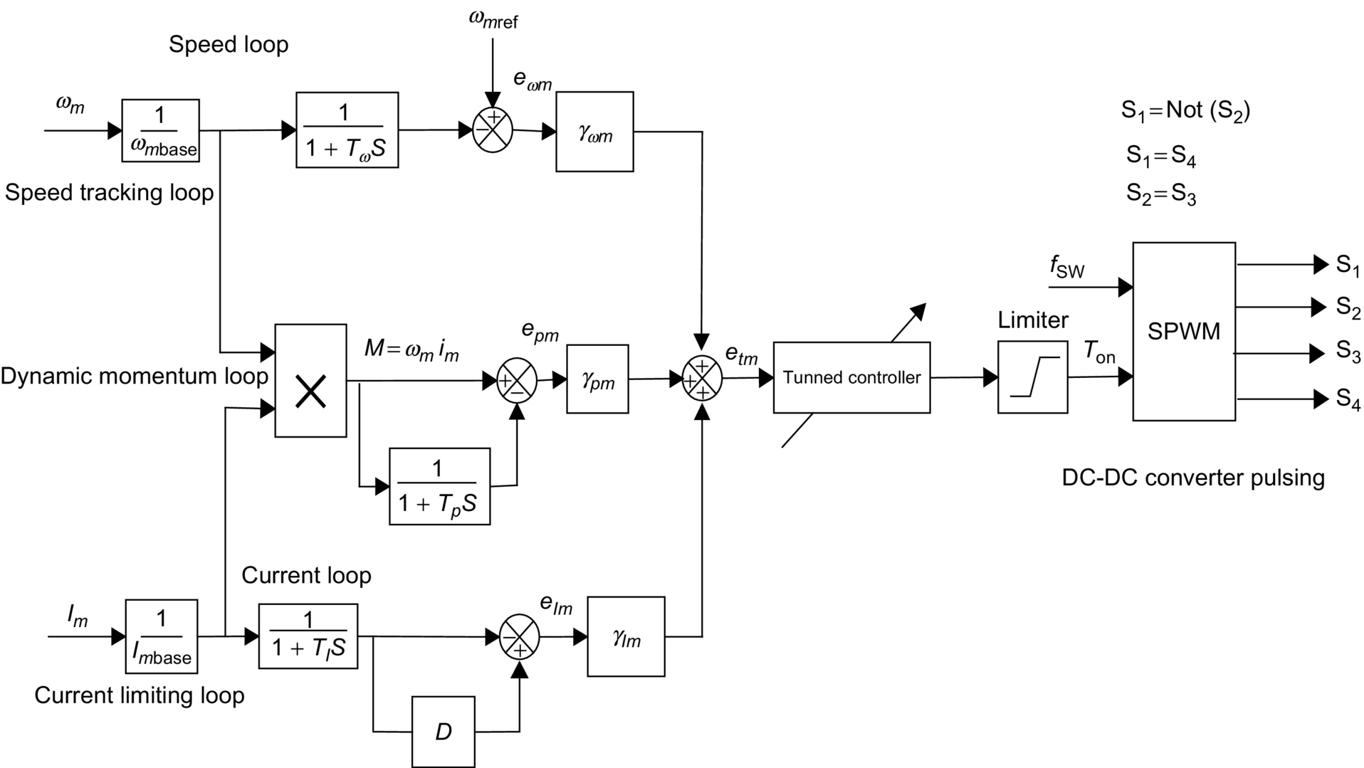
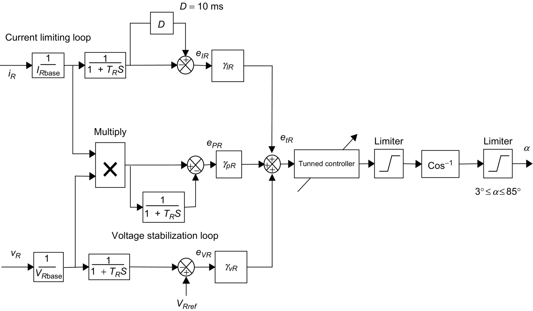
The proposed control system developed by first author comprises four subregulators or controllers named as a diesel DC generator set value control regulator, DC side green plug filter compensator GPFC-SPWM regulator, the permanent magnet DC motor drive speed controller, and the AC/DC power converter regulator. Figs. 38.12–38.15 depict the proposed multiloop dynamic self-regulating controllers based on multiobjective optimization search and optimization technique based on soft computing PSO and GA. The global error is the summation of the three loop individual errors including voltage stability, current limiting, and synthesis dynamic power loops. Each multiloop dynamic control scheme is used to reduce a global error based on a triloop dynamic error summation signal and to mainly track a given speed reference trajectory loop error in addition to other supplementary motor current limiting, and dynamic power loops are used as auxiliary loops to generate a dynamic global total error signal that consists of not only the main loop speed error but also the current ripple, overcurrent limit, and dynamic overload power conditions.
The global error signal is input to the self-tuned controllers shown in Figs. 38.18–38.21. The (per unit) three-dimensional-error vector (evg, eIg, and epg) of the diesel engine controller scheme is governed by the following equations:
evg(k)=Vg(k)(11+STg)(11+SD)−Vg(k)(11+STg)
eIg(k)=Ig(k)(11+STg)(11+SD)−Ig(k)(11+STg)
ePg(k)=Ig(k)×Vg(k)(11+STg)(11+SD)−Ig(k)×Vg(k)(11+STg)


The total or global error etg(k) at the AC side scheme at a time instant
etg(k)=γvgevg(k)+γigeig(k)+γpgepg(k)
In the same manner, the (per unit) three-dimensional-error vector (evd, eId, and epd) of the GPFC scheme is governed by the following equations:
evd(k)=Vd(k)(11+STd)(11+SD)−Vd(k)(11+STd)

eId(k)=Id(k)(11+STd)(11+SD)−Id(k)(11+STd)

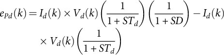
ePd(k)=Id(k)×Vd(k)(11+STd)(11+SD)−Id(k)×Vd(k)(11+STd)
and the total or global error etd(k) for the DC side green plug filter compensator GPFC scheme at a time instant
etd(k)=γvdevd(k)+γideid(k)+γpdepd(k)
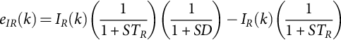
In addition, The (per unit) three-dimensional-error vector (evR, eIR, and epR) of the three-phase-controlled rectifier scheme is governed by the following equations:
evR(k)=VR(k)(11+STR)(11+SD)−VR(k)(11+STR)
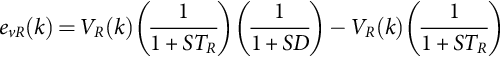
eIR(k)=IR(k)(11+STR)(11+SD)−IR(k)(11+STR)
ePR(k)=IR(k)×VR(k)(11+STR)(11+SD)−IR(k)×VR(k)(11+STR)

The total or global error etR(k) for the three-phase-controlled converter rectifier scheme at a time instant:
etR(k)=γvRevR(k)+γiReiR(k)+γpRepR(k)
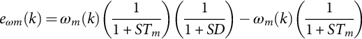
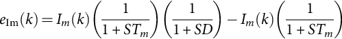
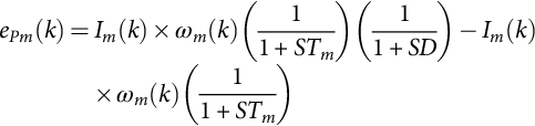
Finally, the (per unit) three-dimensional-error vector (eωm, eIm, and epm) of the PMDC motor scheme is governed by the following equations:
eωm(k)=ωm(k)(11+STm)(11+SD)−ωm(k)(11+STm)
eIm(k)=Im(k)(11+STm)(11+SD)−Im(k)(11+STm)
ePm(k)=Im(k)×ωm(k)(11+STm)(11+SD)−Im(k)×ωm(k)(11+STm)
and the total or global error etm(k) for the MPFC scheme at a time instant
etm(k)=γωmeωm(k)+γimeim(k)+γpmepm(k)
A number of conflicting objective functions are selected to optimize using the PSO algorithm. These functions are defined by the following:
J1=Minimize{|etg|,|etR|,|etd|,|etm|}
J2=Steadystateerror=|eω(k)|=|ωref(k)−ωm(k)|
J3=Settlingtime
J4=Maximumovershoot
J5=Risetime
In general, to solve this multiobjective complex optimality search problem, there are two possible optimization techniques based on particle swarm optimization (PSO): single aggregate selected objective optimization (SOO), which is explained, and multiobjective optimization (MOO). The main procedure of the SOO is based on selecting a single aggregate objective function with weighted single-objective parameters scaled by a number of weighting factors. The objective function is optimized (either minimized or maximized) using either GA or particle swarm optimization search algorithm (PSO) methods to obtain a single global or near-optimal solution. On the other hand, the main objective of the multiobjective (MO) problem is finding the set of acceptable (trade-off) optimal solutions. This set of accepted solutions is called Pareto front. These acceptable trade-off multilevel solutions give more ability to the user to make an informed decision by seeing a wide range of near-optimal selected solutions that are feasible and acceptable from an “overall” standpoint. Single-objective (SO) optimization may ignore this trade-off viewpoint, which is crucial. The main advantages of the proposed MOO method are the following: It doesn't require a priori knowledge of the relative importance of the objective functions, and it provides a set of acceptable trade-off near-optimal solutions. This set is called Pareto front or optimality trade-off surfaces. Both SOO and MOO searching algorithms are tested, validated, and compared. The dynamic error-driven controller regulates the controllers' gains using the particle swarm optimization (PSO) and GA to minimize the system total error, the settling time, the rising time, and the maximum overshoot. The proposed dynamic triloop error-driven controller, developed by the first author, is a novel advanced regulation concept that operates as an adaptive dynamic-type multipurpose controller capable of handling sudden parametric changes, load and/or DC source excursions. By using the triloop error-driven controller, it is expected to have a smoother, less dynamic overshoot and fast and more robust speed controller when compared with those of classical control schemes. The proposed general PMDC motor drive model with the novel triloop error-driven controller is fully validated in this application for effective reference speed trajectory tracking under different loading conditions and parametric variations, such as temperature changes, while driving a complex mechanical load with nonlinear parameters and/or torque-speed characteristics.
Self tuned variable structure sliding mode bang-bang VSC/SMC/B-B controller
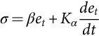
In the variable structure sliding mode controller scheme, an optimally adaptive and self-tuned variable structure sliding mode controller for PMDC motor drive systems using particle swarm optimization technique (PSO) and GA is shown in Fig. 38.22. The slope of the sliding surface is designed as
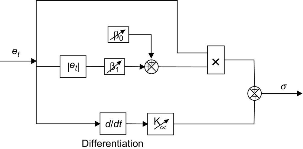
σ=βet+Kαdetdt
With adaptive adjustable error scaling gain,
β=β0+β1|et|
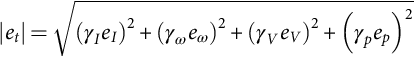
where
|et|=√(γIeI)2+(γωeω)2+(γVeV)2+(γpep)2
The system control voltage has the following form in the time domain [33]: the control is an on-off logic; that is, when σ>0,Vc=1,andwhenσ<0,Vc=−1![]()
The PSO and GA search and optimization are implemented for tuning the various gains β0, β1, and α to minimize the selected five conflicting objective functions (J1−J5). This test is to verify that the proposed VSC/B-B with adaptive β can maintain the motor speed with nonlinear J(ωm) and B(ωm) even if the load changes; accordingly, the robustness can be confirmed.
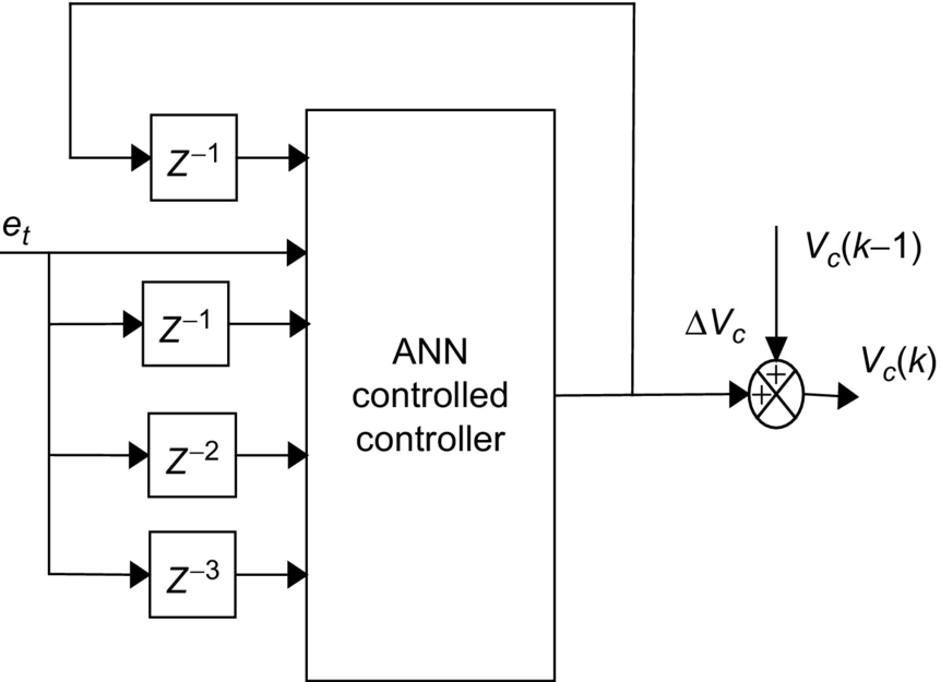
Self tuned artificial neural network controller ANN
The neural network used in this application is the simplest one that uses three layers, which is widely used in the control of the electric machines. Each layer is composed of neurons. Each neuron is connected via weights to the previous layer. The first layer is connected to the input variables. The second one is connected via weights to all the neurons of the previous layer, and the last one is composed of one neuron given the output value. The weights and the biases of the ANN network's are updated to provide that the global error of the system is minimized. The proposed ANN regulator is tuned online using the back-propagation algorithm. The online ANN rule-based algorithm is used to update the ANN network weights and biases to ensure continuous effective dynamic response while keeping the motor inrush current under specified tolerable limits. The input vector with three-layer ANN as shown in Fig. 38.23 is
ˉX={et(k),et(k−1),et(k−2),et(k−3),ΔVc(k−1)}
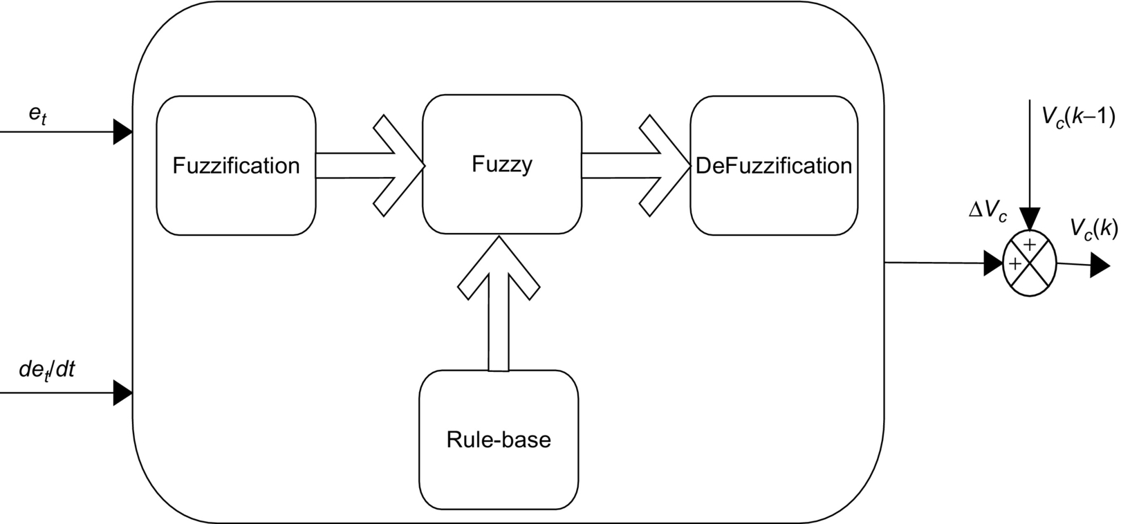
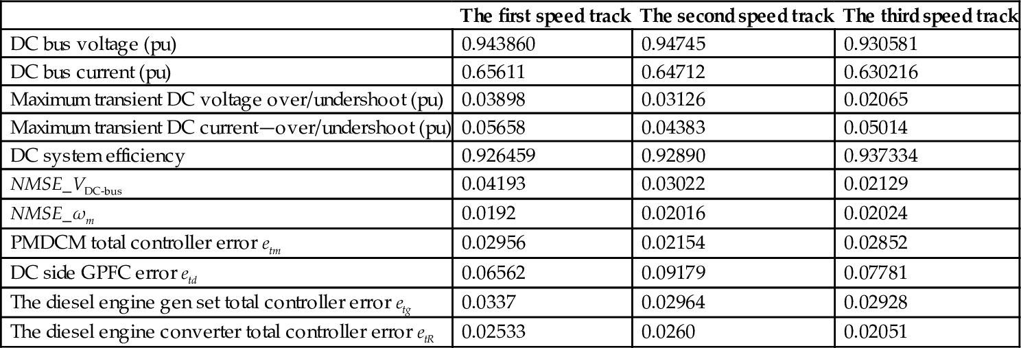
Self tuned fuzzy logic controller (FLC)
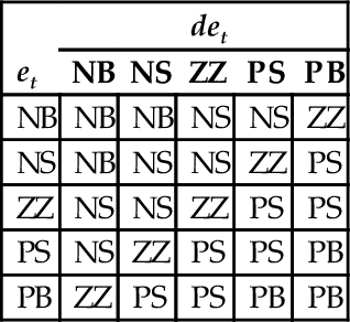
As shown in Fig. 38.24, the FLC system consists of three subsystems, which are the fuzzification, rule base, and defuzzification. Fuzzification subsystem converts the exact inputs to fuzzy values using five membership functions: positive big (PB), positive small (PS), zero (ZZ), negative small (NS), and negative big (NB). The rule base unit processes these fuzzy values with fuzzy rules. The defuzzification unit converts the fuzzy results to exact values. The FLC input values are the global error, et, and change in global error, det. According to these variables, a rule table is produced in the FLC rule base unit as shown in Table 38.4.
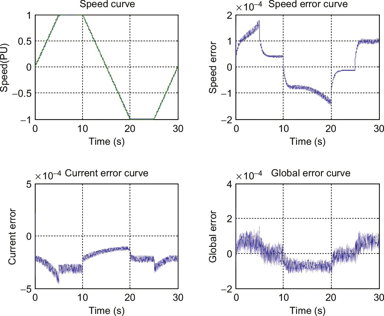
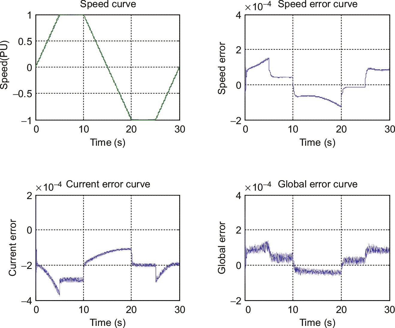
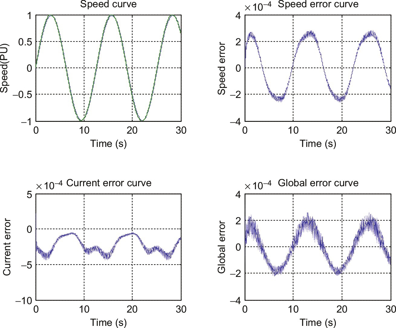
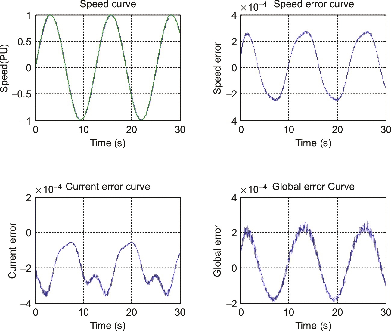
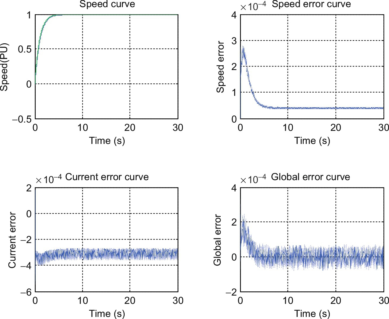
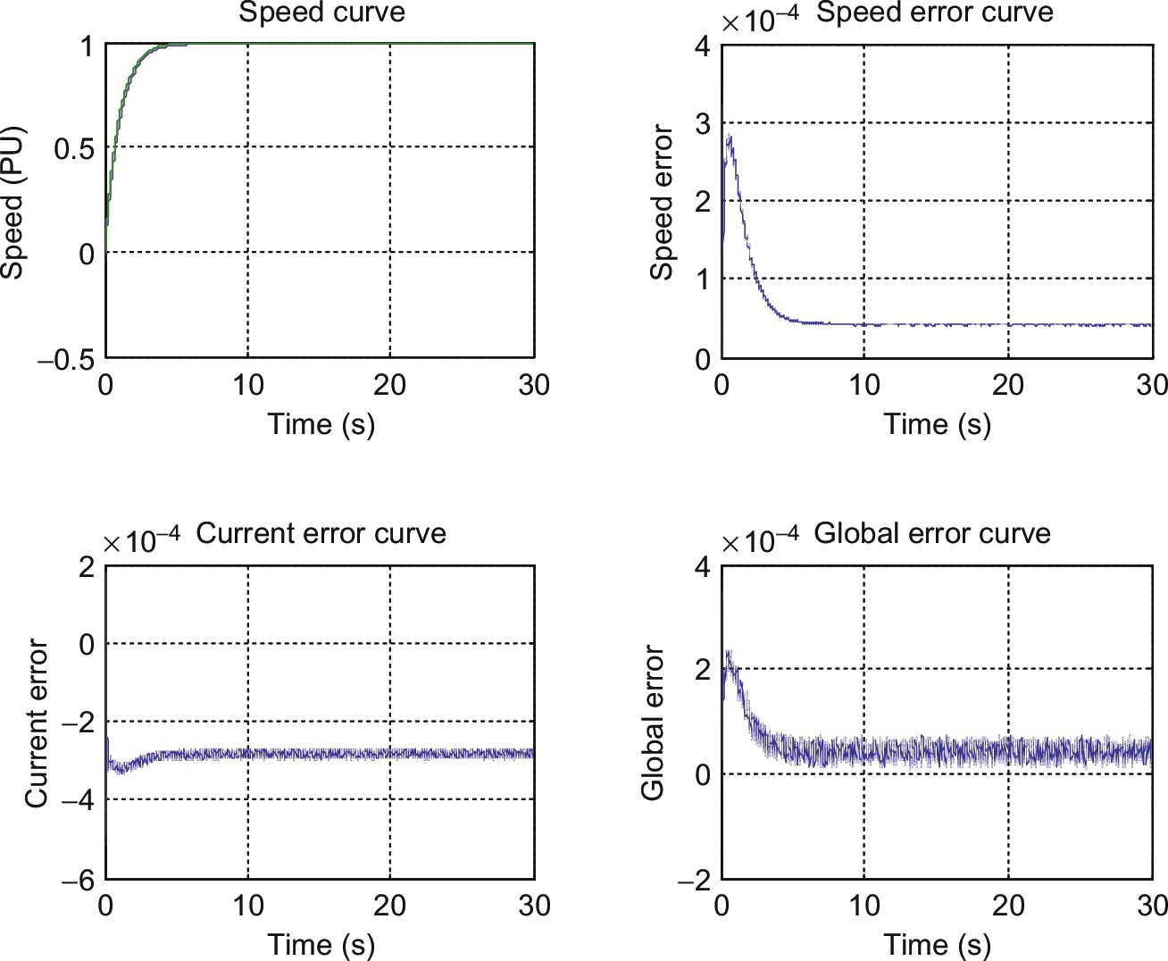
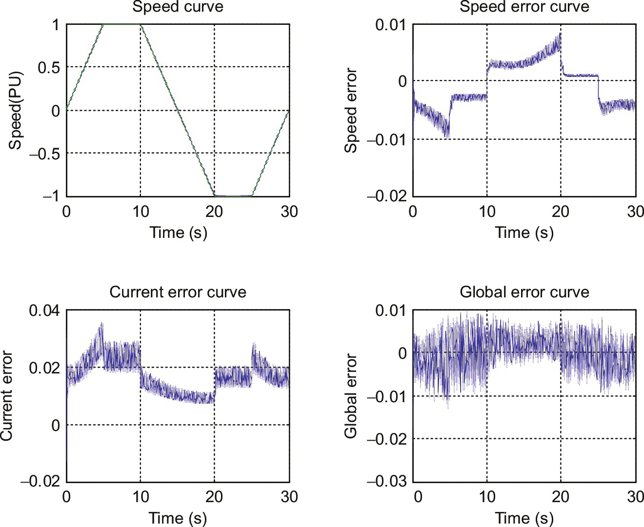
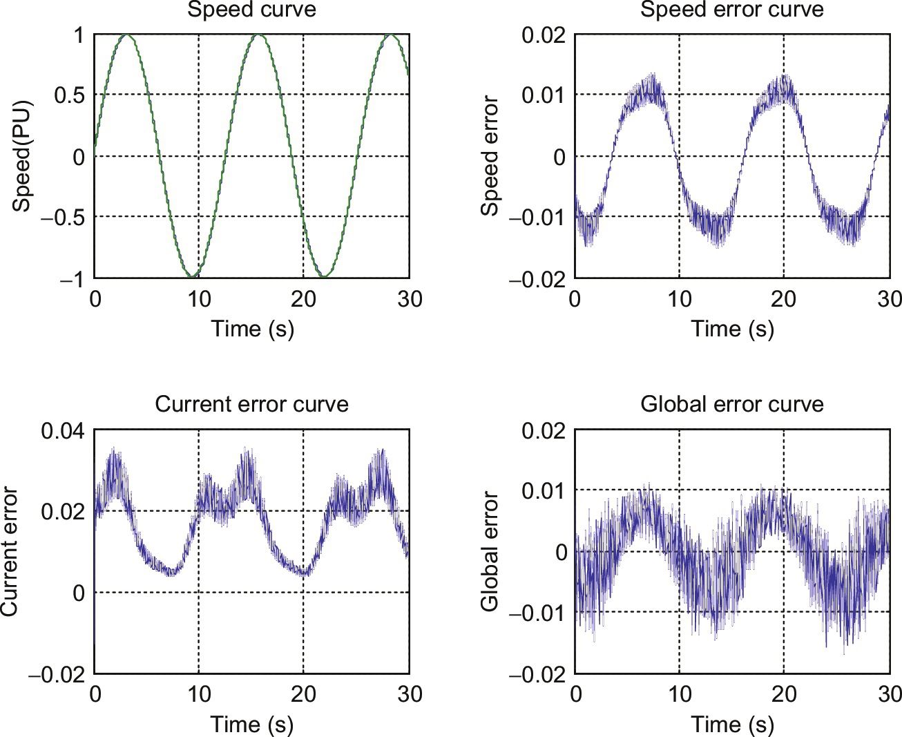
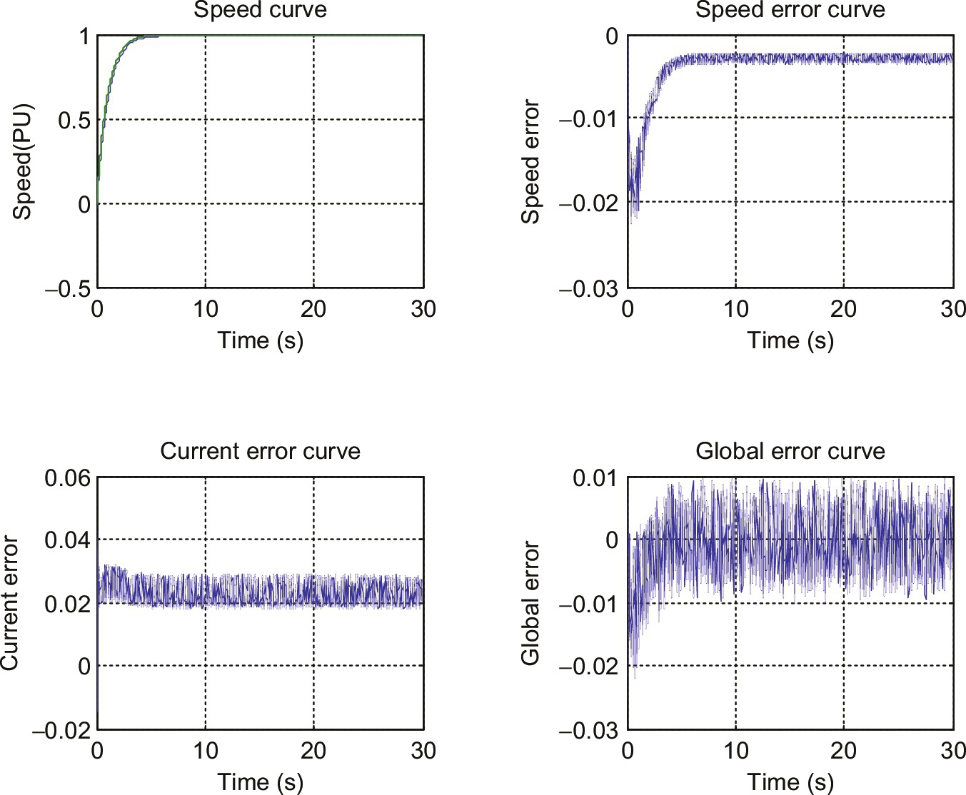
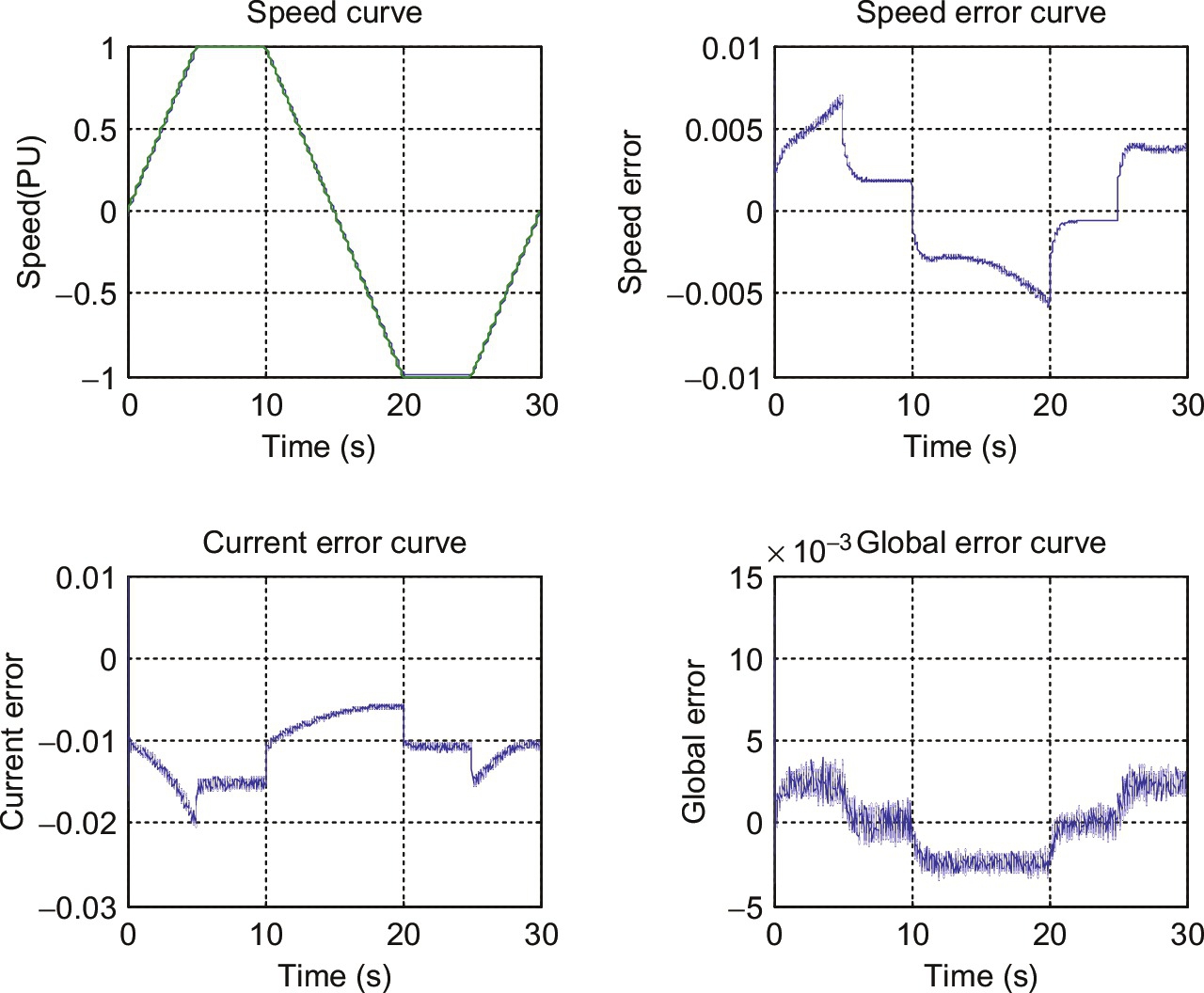
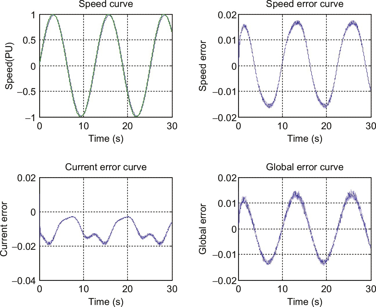
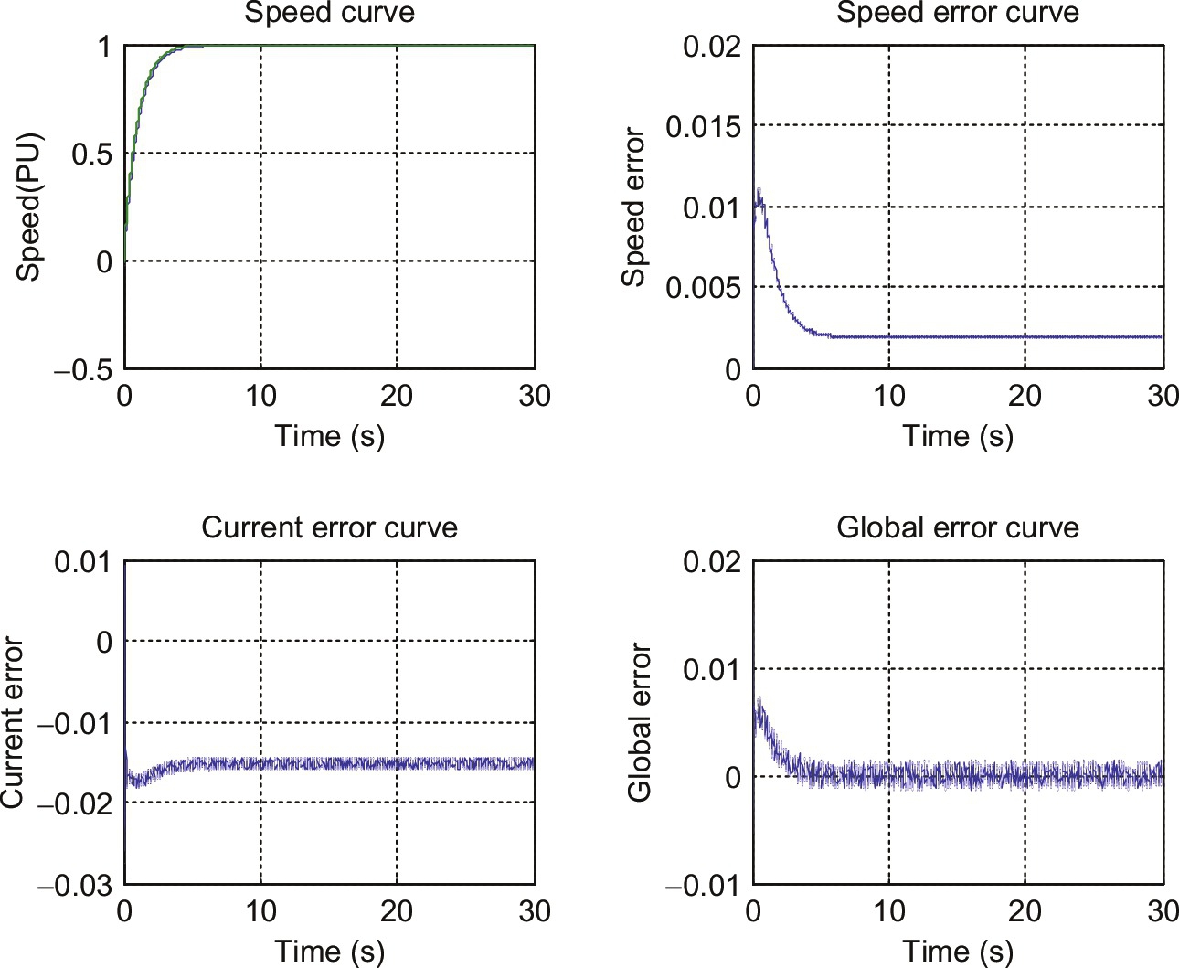
38.8.2.2 Digital Simulation Results
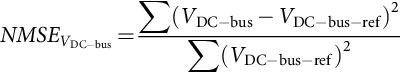
The integrated microgrid for PMDC-driven electric vehicle scheme using the photovoltaic (PV), fuel cell (FC), and backup diesel generation with battery backup renewable generation system performance is compared for two cases, with fixed and self-tuned-type controllers using either GA or PSO. The second case is to compare the performance with artificial neural network (ANN) controller and fuzzy logic controller (FLC) with the self-tuned-type controllers using either GA or PSO. The tuned variable structure sliding mode controller VSC/SMC/B-B has been applied to the speed tracking control of the same EV for performance comparison. There are three different speed references. In the first speed track, the speed increases linearly and reaches the 1 pu at the end of the first 5 s, and then, the reference speed remains speed constant during 5 s. At tenth second, the reference speed decreases with same slope as at the first 5 s. After 15 s, the motor changes the direction and EV increases its speed through the reverse direction. At twentieth second, the reference speed reaches the −1 pu and remains constant speed at the end of twenty-fifth second, and then, the reference speed decreases and becomes zero at thirtieth second. The second reference speed waveform is sinusoidal, and its magnitude is 1 pu, and the period is 12 s. The third reference track is constant speed reference starting with an exponential track. In all references, the system responses have been observed. Matlab/Simulink software was used to design, test, and validate the effectiveness of the integrated microgrid for PMDC-driven electric vehicle scheme using photovoltaic (PV), fuel cell (FC), and backup diesel generation with battery backup renewable generation system with the FACTS devices. The digital dynamic simulation model using Matlab/Simulink software environment allows for low-cost assessment and prototyping, system parameter selection, and optimization of control settings. The use of PSO search algorithm is utilized in online gain adjusting to minimize controller absolute value of total error. This is required before full-scale prototyping that is both expensive and time-consuming. The effectiveness of dynamic simulators brings on detailed submodels selections and tested submodels Matlab library of power system components already tested and validated. The common DC bus voltage reference is set at 1 pu. Digital simulations are obtained with sampling interval Ts=20 μs. Dynamic responses obtained with GA are compared with the ones resulting from the PSO for the seven proposed self-tuned controllers. The dynamic simulation conditions are identical for all tuned controllers. To compare the global performances of all controllers, the normalized mean-square-error (NMSE) deviations between output plant variables and desired values and is defined as
NMSEVDC-bus=∑(VDC-bus−VDC-bus-ref)2∑(VDC-bus-ref)2
NMSEωm=∑(ωm−ωm−ref)2∑(ωm−ref)2
The digital simulation results validated the effectiveness of both GA- and PSO-based tuned controllers in providing effective speed tracking minimal steady-state errors. Transients are also damped with minimal overshoot, settling time, and fall time. The GA- and PSO-based self-tuned controllers are more effective and dynamically advantageous in comparison with the artificial neural network (ANN) controller, the fuzzy logic controller (FLC), and fixed-type controllers. The self-regulation is based on minimal value of absolute total/global error of each regulator shown in Figs. 38.18–38.21. The control system comprising the three dynamic multiloop error-driven regulators is coordinated to minimize the selected objective functions. SOO obtains a single global or near-optimal solution based on a single-weighted objective function. The weighted single-objective function combines several objective functions using specified or selected weighting factors as follows:
weightedobjectivefunction=α1J1+α2J2+α3J3+α4J4+α5J5
where α1=0.20, α2=0.20, α3=0.20, α4=0.20, and α5=0.20 are selected weighting factors. J1, J2, J3, J4, and J5 are the selected objective functions. On the other hand, the MO finds the set of acceptable (trade-off) optimal solutions. This set of accepted solutions is called Pareto front. These acceptable trade-off multilevel solutions give more ability to the user to make an informed decision by seeing a wide range of near-optimal selected solutions.
Table 38.5 shows the optimal solutions of the main objective functions versus the tuned variable structure sliding mode controller gain-based SOGA and MOGA control schemes. On the other hand, Table 38.6 shows the optimal solutions of the main objective functions versus the tuned variable structure sliding mode controller gain-based SOPSO and MOPSO control schemes. Table 38.7 shows the DC bus behavior comparison using the GA-based tuned variable structure sliding mode controller for the three selected reference tracks. In addition, Table 38.8 shows the system behavior using the PSO-based tuned variable structure sliding mode controller. Figs. 38.25–38.30 show the effectiveness of MOPSO and MOGA search and optimized control gains in tracking the PMDC-EV motor three reference speed trajectories. Comparing the PMDC-EV dynamic response results of the two study cases, with GA and PSO tuning algorithms and traditional controllers with constant controller gain results shown in Table 38.9, ANN controller in Table 38.10 (Figs. 38.31–38.33) and FLC in Table 38.11 (Figs. 38.34–38.36), it is quite apparent that the GA and PSO tuning algorithms highly improved the PMDC-EV system dynamic performance from a general power quality point of view. The GA and PSO tuning algorithms had a great impact on the system efficiency improving it from 0.906631 (constant gains controller), 0.928253 (ANN controller), and 0.937334 (FLC) to around 0.948156 (GA-based tuned controller) and 0.930708 (PSO-based tuned controller) that is highly desired. Moreover, the normalized mean square error (NMSE-VDC-Bus) of the DC bus voltage is reduced from 0.08443 (constant gains controller), 0.04827 (ANN controller), and 0.03022 (FLC) to around 0.007304 (GA-based tuned controller) and 0.005854 (PSO-based tuned controller). In addition, the normalized mean square error (NMSE_ωm) of the PMDC motor is reduced from 0.053548 (constant gains controller), 0.02627 (ANN controller), and 0.02016 (FLC) to around 0.0076308 (GA-based tuned controller) and 0.006309 (PSO-based tuned controller). Maximum transient DC voltage over/undershoot (pu) is reduced from 0.054604 (constant gains controller), 0.04186 (ANN controller), and 0.03126 (FLC) to around 0.009302 (GA-based tuned controller) and 0.007259 (PSO-based tuned controller). Maximum transient DC current—over/undershoot (pu) is reduced from 0.087336 (constant gains controller), 0.07355 (ANN controller), and 0.04383 (FLC) to around 0.00292 (GA-based tuned controller) and 0.005987 (PSO-based tuned controller). DC bus voltage (pu) is improved from 0.917020 (constant gains controller), 0.932736 (ANN controller), and 0.94745 (FLC) to around 0.97417 (GA-based tuned controller) and 0.974602 (PSO-based tuned controller). DC bus current (pu) is reduced from 0.769594 (constant gains controller), 0.67464 (ANN controller), and 0.64712 (FLC) to around 0.614695 (GA-based tuned controller) and 0.607674 (PSO-based tuned controller). PMDCM total controller Error (etm) is reduced from 0.095145 (constant gains controller), 0.04200 (ANN controller), and 0.02154 (FLC) to around 0.009167 (GA-based tuned controller) and 0.0048638 (PSO-based tuned controller). DC side GPFC Error (etd) is reduced from 0.70746 (constant gains controller), 0.03416 (ANN controller), and 0.02416 (FLC) to around 0.004618 (GA-based tuned controller) and 0.0074294 (PSO-based tuned controller). The diesel engine gen set total controller error (etg) is reduced from 0.067513 (constant gains controller), 0.04507 (ANN controller), and 0.02964 (FLC) to around 0.005121 (GA-based tuned controller) and 0.007013 (PSO-based tuned controller). The diesel engine converter total controller error (etR) is reduced from 0.086233 (constant gains controller), 0.03978 (ANN controller), and 0.0260 (FLC) to around 0.003265 (GA-based tuned controller) and 0.0053836 (PSO-based tuned controller).
Table 38.5
Selected objective functions versus the tuned variable structure sliding mode controller-based SOGA and MOGA control schemes
| The diesel generator regulator [Kαgβ0gβ1g] |
The GPFC-DC side regulator [Kαdβ0dβ1d] |
The PMDC motor regulator [Kαmβ0mβ1m] |
The α- controller for the converter regulator [KαRβ0Rβ1R] |
J1 Minimize the (total error) ×10−2 |
J2 Minimize the (steady-state error) (pu) ×10−2 |
J3 Minimize the (settling time) (pu) ×10−2 |
J4 Minimize the (maximum overshoot) ×10−2 |
J5 Minimize the (rise time) ×10−2 | |
| SOGA | 0.4111 | 0.6814 | 0.5376 | 0.0775 | 0.4262 | 0.9659 | 0.3315 | 0.6058 | 0.4274 |
| 7.6052 | 7.2686 | 3.7351 | 2.3320 | ||||||
| 34.4595 | 18.0903 | 20.3967 | 49.4889 | ||||||
| MOGA | 0.2438 | 0.1278 | 0.5250 | 0.7085 | 0.3359 | 0.1214 | 0.1330 | 0.6465 | 0.5219 |
| 6.7638 | 9.9706 | 4.6294 | 2.0195 | ||||||
| 39.6771 | 41.6427 | 29.9333 | 31.7174 | ||||||
| 0.4171 | 0.7711 | 0.0017 | 0.8023 | 0.6439 | 0. 5840 | 0.8680 | 0.5505 | 0.4381 | |
| 9.9078 | 7.3238 | 7.2307 | 6.6139 | ||||||
| 42.8415 | 30.3825 | 41.9151 | 33.9013 | ||||||
| 0.0796 | 0.5655 | 0.9480 | 0.5227 | 0.9325 | 0.7425 | 0.1286 | 0.4502 | 0.1956 | |
| 4.6150 | 9.8655 | 8.5251 | 9.5619 | ||||||
| 14.8331 | 27.3988 | 20.8308 | 27.8837 | ||||||
| 0.5943 | 0.8238 | 0.8155 | 0.3747 | 0. 6220 | 0.8159 | 0.7435 | 0.3811 | 0.8706 | |
| 2.5467 | 9.8989 | 2.4722 | 5.2401 | ||||||
| 14.8681 | 13.7004 | 37.7790 | 42.9201 | ||||||
| 0.8499 | 0.9512 | 0.2953 | 0.4528 | 0.8135 | 0.2985 | 0.1727 | 0.4810 | 0. 7690 | |
| 5.2918 | 2.8911 | 6.2706 | 8.2844 | ||||||
| 40.0583 | 30.3251 | 45.0299 | 22.0045 | ||||||
| 0.7103 | 0.0042 | 0.3397 | 0.3788 | 0.6970 | 0.7092 | 0.4680 | 0.3245 | 0.8129 | |
| 5.8841 | 9.0935 | 8.5068 | 7.4244 | ||||||
| 13.7034 | 26.9887 | 27.6030 | 33.5903 |
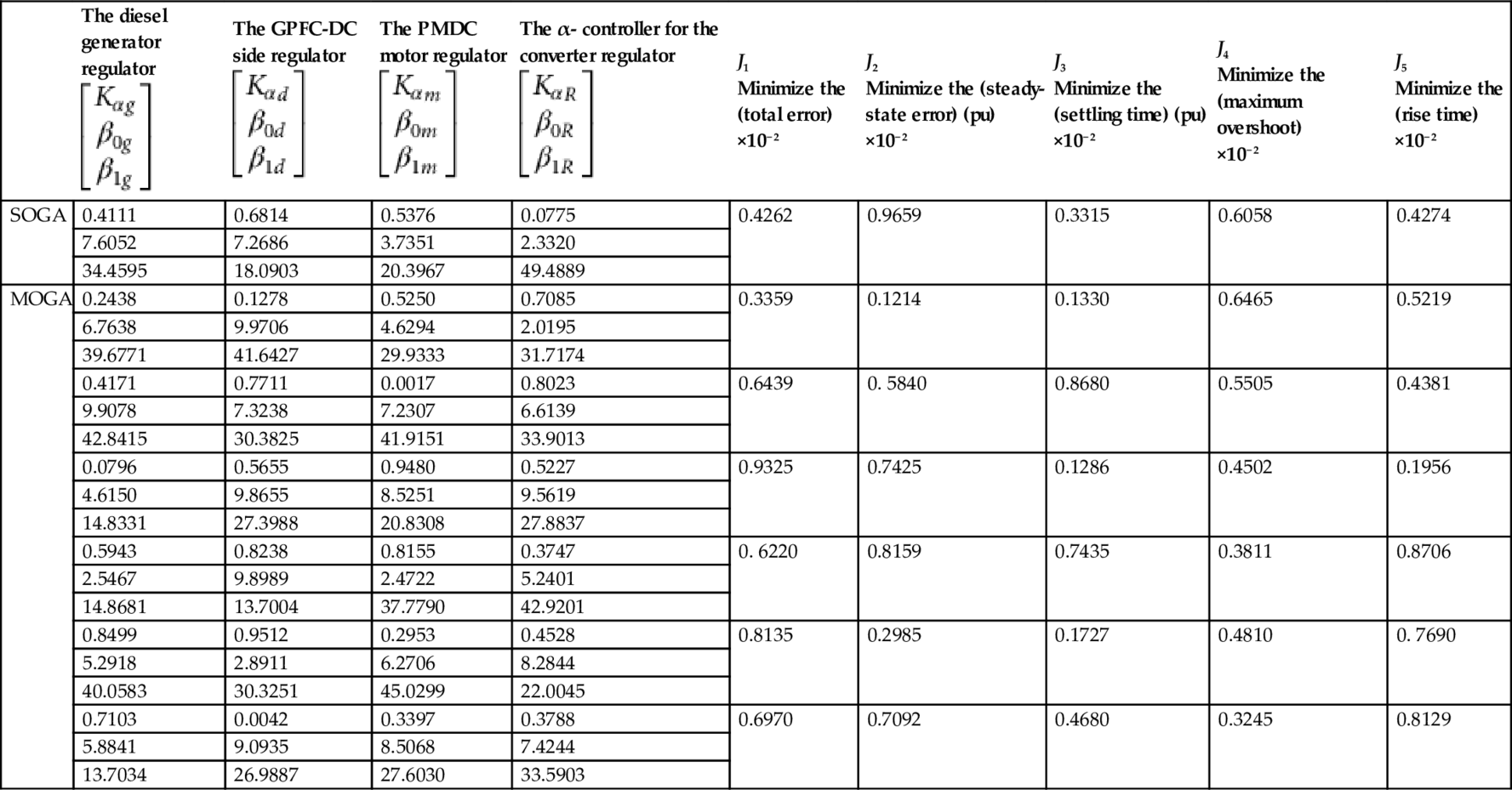
Table 38.6
Selected objective functions versus the tuned variable structure sliding mode controller gains based SOPSO and MOPSO control schemes
| The Diesel generator Regulator [Kαgβ0gβ1g] |
The GPFC – DC side Regulator [Kαdβ0dβ1d] |
The PMDC motor Regulator [Kαmβ0mβ1m] |
the α- controller for the converter Regulator [KαRβ0Rβ1R] |
J1 Minimize the (Total Error) ×10−2 |
J2 Minimize the (Steady State Error) (PU) ×10−2 |
J3 Minimize the (Settling Time) (PU) ×10−2 |
J4 Minimize the (Maximum Overshoot) ×10−2 |
J5 Minimize the (Rise Time) ×10−2 | |
| SOPSO | 0.6420 | 0.8224 | 0.4837 | 0.9958 | 0.6430 | 0.5063 | 0.3271 | 0.2178 | 0.1942 |
| 3.5994 | 4.5435 | 1.5718 | 4.7632 | ||||||
| 15.9501 | 45.8496 | 30.2713 | 38.4880 | ||||||
| MOPSO | 0.9180 | 0.1091 | 0.9511 | 0.2032 | 0.1188 | 0.4657 | 0.8187 | 0.7850 | 0.6490 |
| 6.8088 | 7.1060 | 5.3405 | 3.3284 | ||||||
| 41.9628 | 26.4457 | 33.8367 | 26.9778 | ||||||
| 0.7877 | 0.6885 | 0.4439 | 0.4364 | 0.6431 | 0.6374 | 0.4381 | 0.3956 | 0.1433 | |
| 8.2403 | 6.4446 | 9.0896 | 5.2320 | ||||||
| 33.1334 | 45.6199 | 26.3367 | 19.1299 | ||||||
| 0.2735 | 0.5283 | 0.4714 | 0.6509 | 0.7553 | 0.1289 | 0.5451 | 0.7768 | 0.3175 | |
| 8.0252 | 9.0582 | 4.1808 | 5.1085 | ||||||
| 25.5645 | 47.8210 | 19.7245 | 49.4370 | ||||||
| 0.6223 | 0.2945 | 0.0753 | 0.5513 | 0.7700 | 0.5610 | 0.5095 | 0.3739 | 0.5064 | |
| 6.1631 | 3.5565 | 5.5806 | 5.3880 | ||||||
| 35.5179 | 44.9276 | 33.6105 | 40.9104 | ||||||
| 0.7421 | 0.5091 | 0.8113 | 0.5772 | 0.8056 | 0.2506 | 0.4081 | 0.7742 | 0.2081 | |
| 8.5694 | 4.4184 | 3.9733 | 5.9874 | ||||||
| 17.4213 | 35.7326 | 46.4878 | 27.2446 | ||||||
| 0.8711 | 0.0135 | 0.5838 | 0.7024 | 0.5603 | 0.3070 | 0.6489 | 0.1938 | 0.3129 | |
| 7.2711 | 4.0452 | 8.5443 | 1.7882 | ||||||
| 17.0029 | 26.1268 | 30.2219 | 17.1486 |
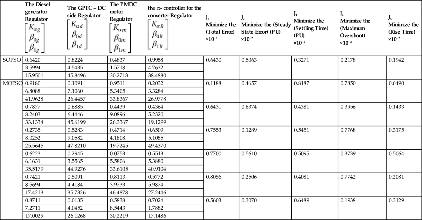
Table 38.7
DC bus behavior comparison using the GA-based tuned variable structure sliding mode controller VSC/SMC/B-B
| The first speed track | The second speed track | The third speed track | |
| DC bus voltage (pu) | 0.964652 | 0.97417 | 0.964182 |
| DC bus current (pu) | 0.60878 | 0.614695 | 0.613914 |
| Maximum transient DC voltage over/undershoot (pu) | 0.0085931 | 0.009302 | 0.008437 |
| Maximum transient DC current—over/undershoot (pu) | 0.002005 | 0.00292 | 0.0028122 |
| DC system efficiency | 0.9404 | 0.948156 | 0.94302 |
| NMSE_VDC-bus | 0.0073133 | 0.007304 | 0.008248 |
| NMSE_ωm | 0.0074627 | 0.0076308 | 0.008558 |
| PMDCM total controller error etm | 0.008187 | 0.009167 | 0.007663 |
| DC side GPFC error etd | 0.003062 | 0.004618 | 0.004337 |
| The diesel engine gen set total controller error etg | 0.0047025 | 0.005121 | 0.004377 |
| The diesel engine converter total controller error etR | 0.002879 | 0.003265 | 0.002328 |
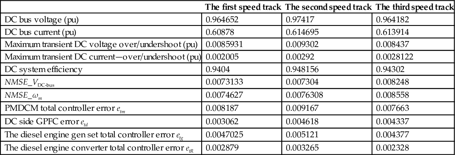
Table 38.8
DC bus behavior comparison using the PSO-based tuned variable structure sliding mode controller VSC/SMC/B-B
| The first speed track | The second speed track | The third speed track | |
| DC bus voltage (pu) | 0.97347 | 0.974602 | 0.950341 |
| DC bus current (pu) | 0.604077 | 0.607674 | 0.605076 |
| Maximum transient DC voltage over/undershoot (pu) | 0.0073109 | 0.007259 | 0.008571 |
| Maximum transient DC current—over/undershoot (pu) | 0.004746 | 0.005987 | 0.0047885 |
| DC system efficiency | 0.932558 | 0.930708 | 0.9327892 |
| NMSE_VDC-bus | 0.004941 | 0.005854 | 0.0052055 |
| NMSE_ωm | 0.0065287 | 0.006309 | 0.007071 |
| PMDCM total controller error etm | 0.005095 | 0.0048638 | 0.0052238 |
| DC side GPFC error etd | 0.0072358 | 0.0074294 | 0.007769 |
| The diesel engine gen set total controller error etg | 0.0069206 | 0.007013 | 0.0071823 |
| The diesel engine converter total controller error etR | 0.005167 | 0.0053836 | 0.0052152 |
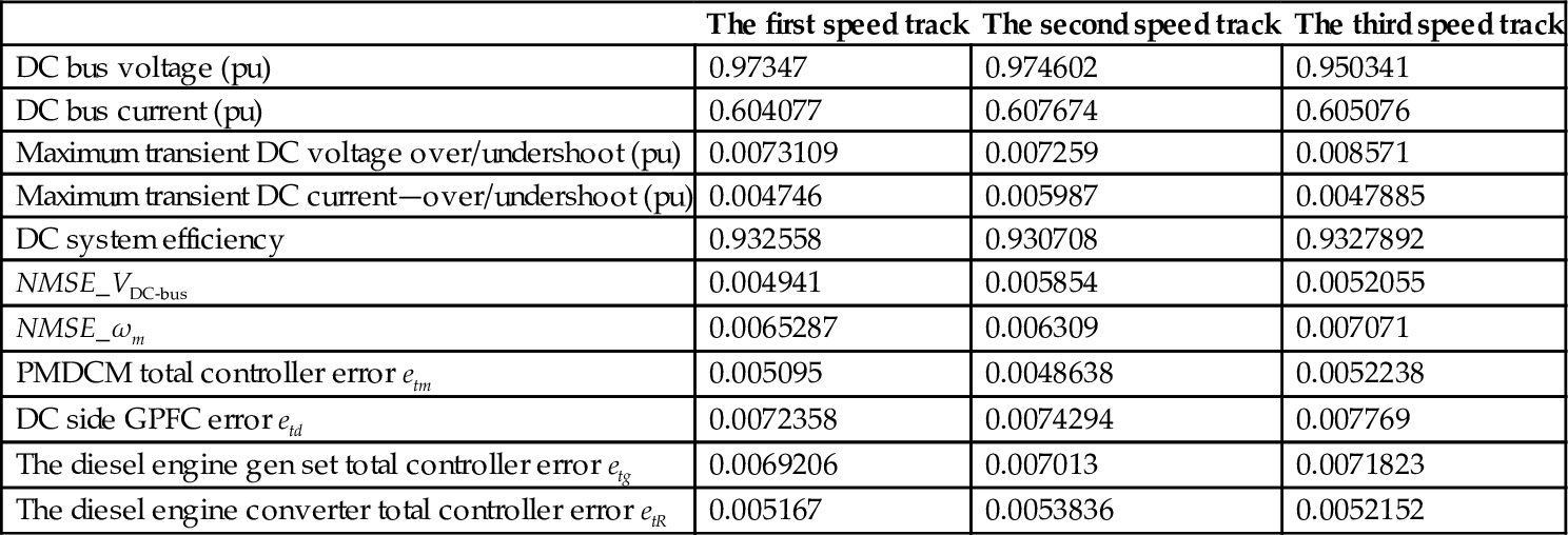
Table 38.9
DC bus behavior comparison using the constant parameter variable structure sliding mode controller VSC/SMC/B-B
| The first speed track | The second speed track | The third speed track | |
| DC bus voltage (pu) | 0.904060 | 0.917020 | 0.895291 |
| DC bus current (pu) | 0.76545 | 0.769594 | 0.769731 |
| Maximum transient DC voltage over/undershoot (pu) | 0.052925 | 0.054604 | 0.053089 |
| Maximum transient DC current—over/undershoot (pu) | 0.09461 | 0.087336 | 0.081906 |
| DC system efficiency | 0.885737 | 0.906631 | 0.895666 |
| NMSE_VDC-bus | 0.09512 | 0.08443 | 0.084672 |
| NMSE_ωm | 0.05131 | 0.053548 | 0.053953 |
| PMDCM total controller error etm | 0.08521 | 0.095145 | 0.09422 |
| DC side GPFC error etd | 0.072338 | 0.70746 | 0.703462 |
| The diesel engine gen set total controller error etg | 0.062513 | 0.067513 | 0.069606 |
| The diesel engine converter total controller error etR | 0.08856 | 0.086233 | 0.085740 |
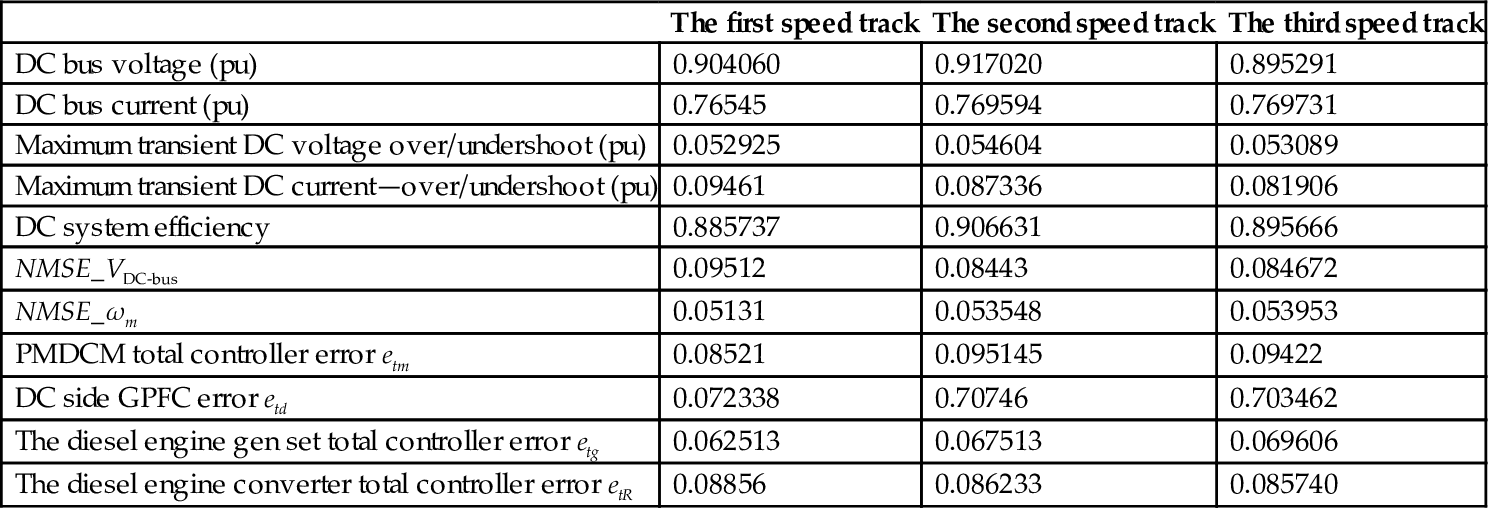
Table 38.10
DC bus behavior comparison using ANN controller
| The first speed track | The second speed track | The third speed track | |
| DC bus voltage (pu) | 0.92747 | 0.932736 | 0.91131 |
| DC bus current (pu) | 0.661466 | 0.67464 | 0.64627 |
| Maximum transient DC voltage over/undershoot (pu) | 0.0372 | 0.04186 | 0.05541 |
| Maximum transient DC current—over/undershoot (pu) | 0.08575 | 0.07355 | 0.06083 |
| DC system efficiency | 0.916100 | 0.928253 | 0.926261 |
| NMSE_VDC-bus | 0.03439 | 0.04827 | 0.05231 |
| NMSE_ωm | 0.03793 | 0.02627 | 0.03146 |
| PMDCM total controller error etm | 0.04261 | 0.04200 | 0.04639 |
| DC side GPFC error etd | 0.02397 | 0.02416 | 0.02440 |
| The diesel engine gen set total controller error etg | 0.04437 | 0.04507 | 0.05522 |
| The diesel engine converter total controller error etR | 0.03388 | 0.03978 | 0.03463 |
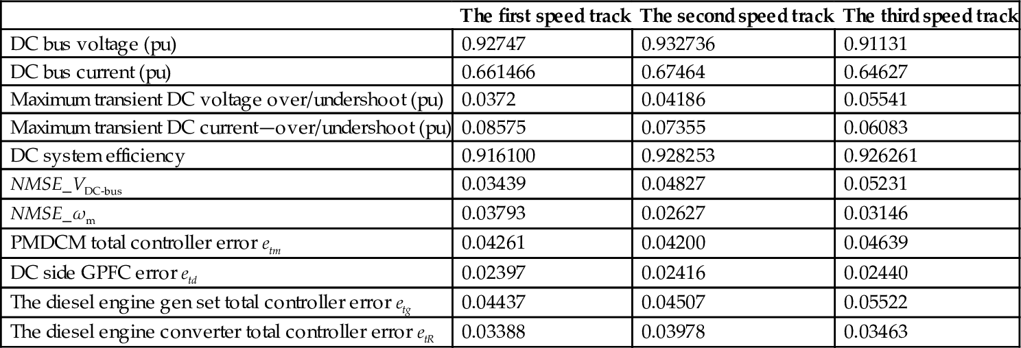
Table 38.11
DC bus behavior comparison using FLC controller
| The first speed track | The second speed track | The third speed track | |
| DC bus voltage (pu) | 0.943860 | 0.94745 | 0.930581 |
| DC bus current (pu) | 0.65611 | 0.64712 | 0.630216 |
| Maximum transient DC voltage over/undershoot (pu) | 0.03898 | 0.03126 | 0.02065 |
| Maximum transient DC current—over/undershoot (pu) | 0.05658 | 0.04383 | 0.05014 |
| DC system efficiency | 0.926459 | 0.92890 | 0.937334 |
| NMSE_VDC-bus | 0.04193 | 0.03022 | 0.02129 |
| NMSE_ωm | 0.0192 | 0.02016 | 0.02024 |
| PMDCM total controller error etm | 0.02956 | 0.02154 | 0.02852 |
| DC side GPFC error etd | 0.06562 | 0.09179 | 0.07781 |
| The diesel engine gen set total controller error etg | 0.0337 | 0.02964 | 0.02928 |
| The diesel engine converter total controller error etR | 0.02533 | 0.0260 | 0.02051 |
38.8.3 Novel Self Regulating Green Plug/Energy Management/Energy Economizer GP-EM-EE Schemes for Wind Driven Induction Generation
The application presents a novel self-adjusting wind energy utilization scheme using a modified single-phase operation of the three-phase induction generator supplemented by a voltage stabilization switched filter compensation scheme developed by the first author. The series-parallel switched capacitor filter scheme is controlled by a dynamic particle swarm optimization (PSO) and GA error-driven self-adjusting controller to ensure voltage stabilization, minimum impact of the electric load excursions, and wind variations on terminal voltage. The sinusoidal pulse-width modulation complementary switching scheme is dynamically controlled using online minimal global error search that continuously adjusts and modifies the controller gains. The application presents a family of novel switched smart filter compensated devices using green plug/energy management/energy economizer GP-EM-EE devices for small single-phase induction motors used in residential/commercial motor drives used in water pumping, ventilation, air conditioning, compressors, and refrigeration applications. The GP-EM-EE devices are equipped with a dynamic online error-driven optimally tuned controller that ensures improved power factor, reduced feeder losses, stabilized voltage, minimal current ripples, and efficient energy utilization/conservation with minimal impact on the host electric grid security and reliability. The proposed schemes can enhance the power quality and extend induction motor life span by reducing overheating due to inrush currents and harmonics. They prevent overheating and possible motor damage. The scheme is suitable for small-scale applications of wind energy utilization in the range from 5 to 25 kVA.
Wind energy conversion systems (WECS) are increasing their number as an environmentally friendly power generation system. Small-sized wind turbine systems in the output power range of 5–25 kVA to be used for the residential houses or small-sized business complex are extending their application fields. There are various advantages of the small-sized wind turbine system. The rotational speed of the smaller sized wind turbines can more rapidly follow the change of the wind speed than the large-scale wind turbines system due to their smaller inertia. This feature contributes higher power generation efficiency of the wind turbines in the case that the wind speed frequently changes [34]. Induction generators are being increasingly utilized in a WECS since they are relatively inexpensive, rigid, and require low maintenance [35]. Small-scale induction motor drives consume over 50% of the total electric energy generated in the developed countries [36]. The electric utility industry and consumers of electric energy around the world are facing new challenges for cutting electric energy cost, improving energy utilization, enhancing energy efficiency, demand-side management, improving supply waveform power quality, reducing safety hazards to personnel, and protecting sensitive computer and automatic data processing networks [37]. There is a mushrooming use of nonlinear electric loads especially in large motor drives, arc furnaces, and power electronic converter loads. All these nonlinear loads are by-products of analog (saturation or limiter-type) or digital (converter, solid-state switching-type) nonlinearities [38]. Nonlinear-type loads cause severe waveform distortion, power quality problem interference, and extra feeder losses due to excessive inrush currents and severe voltage sags. The extended use of power electronic switching conveners and devices in motor drives and process industries such as mining, oil, and gas industries and industrial DC and AC arc-type furnaces has resulted in a polluted grid and unreliable radial distribution/utilization system with serious inherent voltage and power quality problems [39]. These nonlinear-type electric loads are used with ventilation, air conditioning, water pumping, and low-power factor industries such as sewing, printing, shear and press machinery, and food processing plants. These nonlinear loads also fall in the category of inrush or arc-type motorized loads and combined with fluorescent lighting can cause waveform distortion, harmonic interference, and voltage flickering [40–42]. Generally, direct online motor starting is an economic method for starting induction motors. But direct starting will result in severe voltage sags and extra heating. When starting large induction motors, excessive voltage dips result in overheating and loss of motor life expectancy [43].
38.8.3.1 Sample Study Motorized System
Fig. 38.37 depicts the block diagram of the utilization (single-phase induction motor SPIM) and the connection of switched smart filter compensated device using green plug/energy management/energy economizer GP-EM-EE devices and the speed control drive system to the SPIM load. Figs. 38.38 and 38.39 show the proposed triloop dynamic tracking controller to ensure both objectives of (energy/power) saving and power quality enhancement of the supply system current and load bus voltage. The novel PSO and GA self-tuned multiregulators and coordinated controller are used for the following purposes: (1) green plug filter compensator GPFC-SPWM regulator for pulse-width switching scheme to regulate the DC bus voltage and minimize inrush current transients and load excursions and (2) the SPIM drive with the speed regulator that ensures speed reference tracking with minimum inrush conditions and ensure reduced voltage transients and improved energy utilization. Figs. 38.40–38.44 depict the proposed family of switched smart filter compensated devices using green plug/energy management/energy economizer GP-EM-EE devices. All filters objectives can be either (a) harmonic reduction and power quality (PQ) enhancement or (b) electric power/energy savings and dynamic reactive compensation for the single-phase induction motor loads. The proposed utilization scheme is fully validated using the Matlab/Simulink software environment under normal conditions, load excursion, SPIM motor torque changes to assess the control system robustness, effective energy utilization, and speed reference tracking.
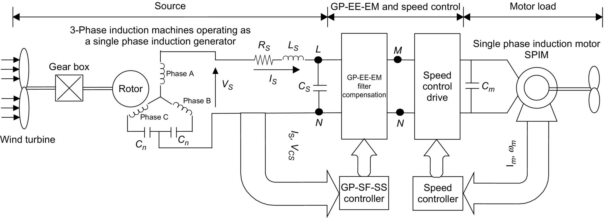
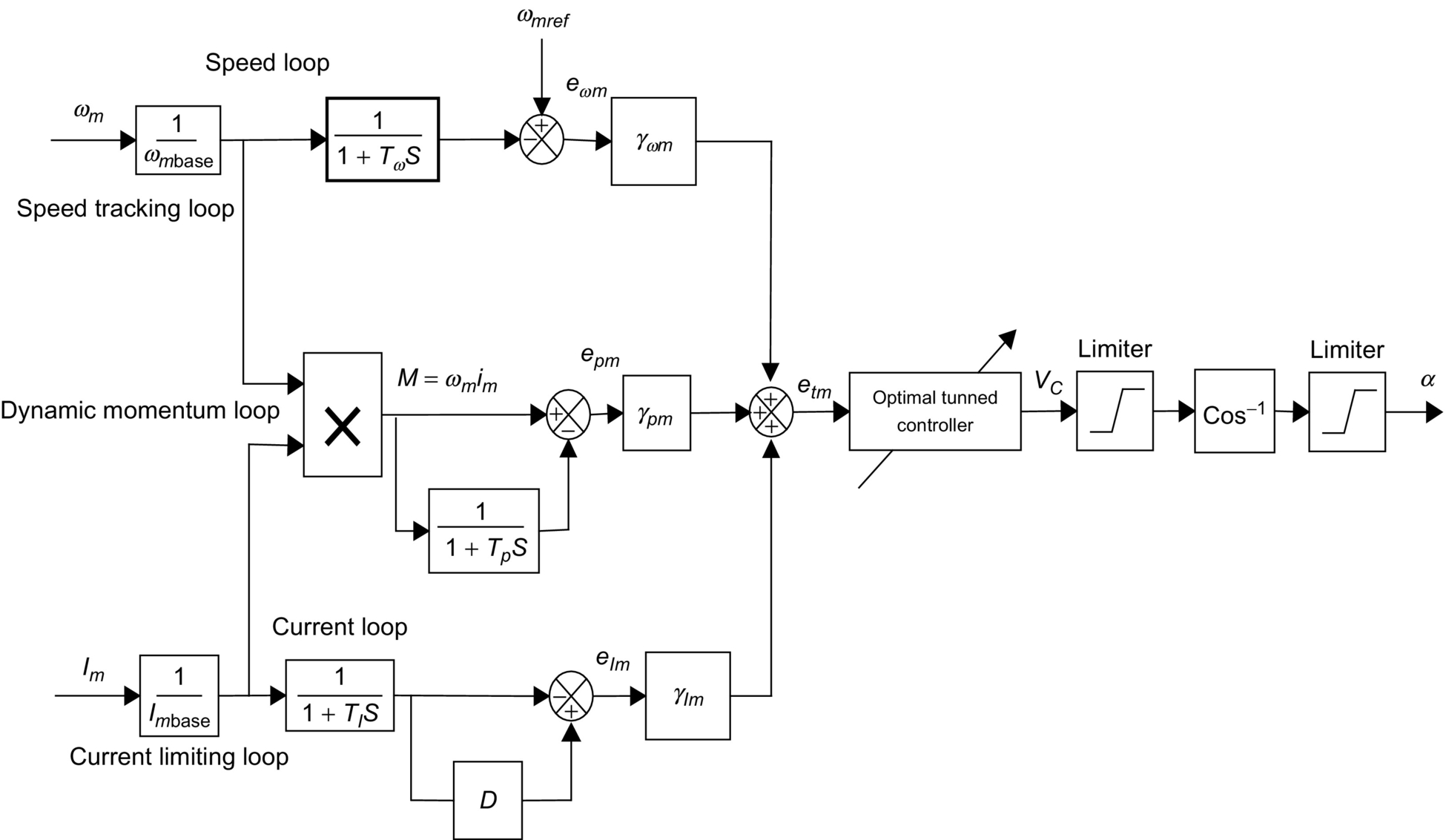
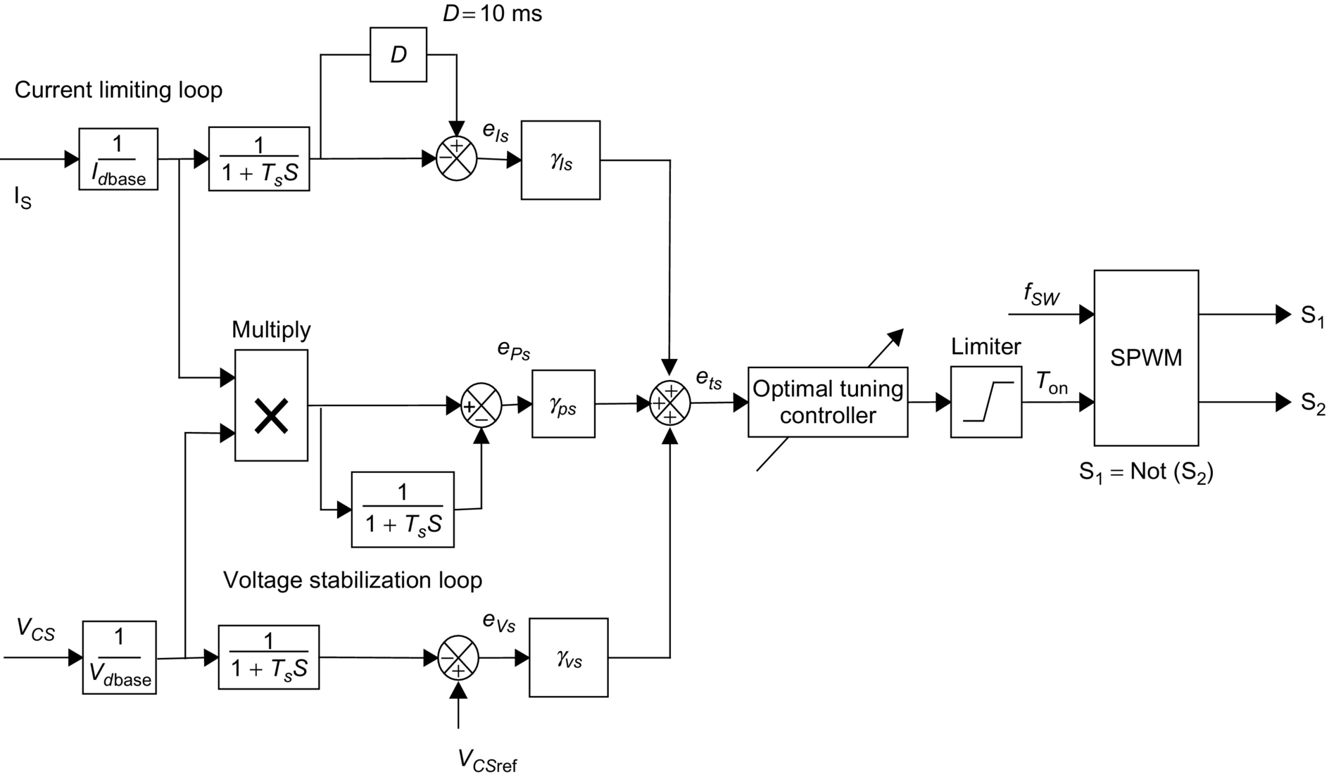
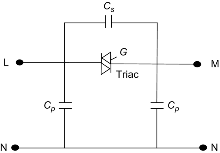
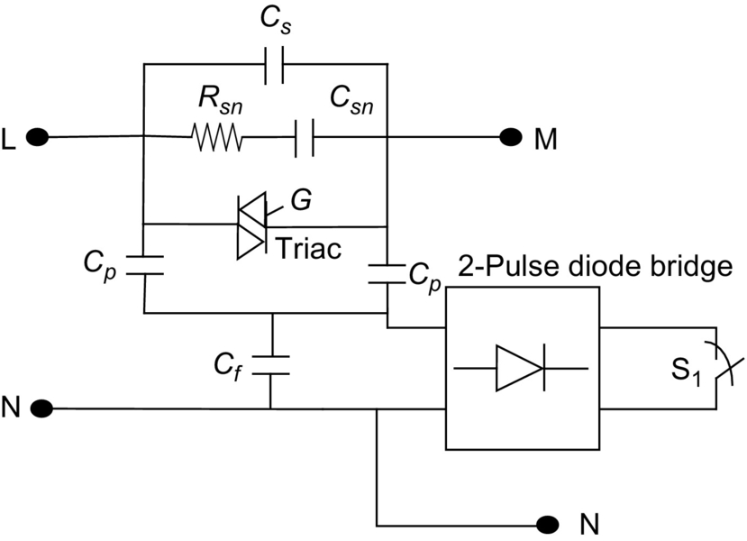
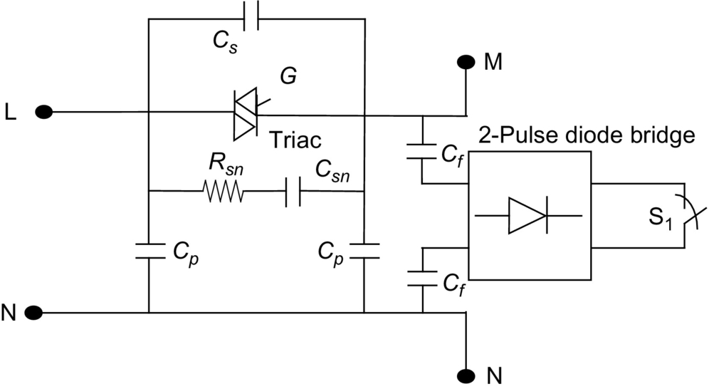
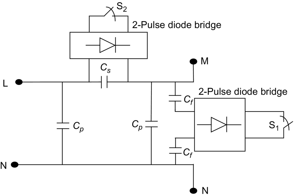
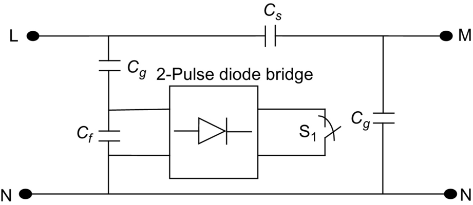
The common concerns of power quality are the long-duration voltage variations (overvoltage, undervoltage, and sustained interruptions), short-duration voltage variations (interruption, sags, and swells), voltage imbalance (voltage unbalance), waveform distortion (DC offset, harmonics, interharmonics, notching, and noise), voltage fluctuation (voltage flicker), and power frequency variations. To prevent the undesirable states and to reduce the power consumption, a GPF scheme is used to stabilize the system.
Dynamic error driven control
The proposed control system comprises two subregulators or controllers named as DC side green plug filter compensator GPFC-SPWM regulator and the SPIM drive speed controller. Figs. 38.38 and 38.39 depict the proposed multiloop dynamic self-regulating controllers based on multiobjective optimization search and optimization technique based on soft computing PSO and GA. The global error is the summation of the three loop individual errors including voltage stability, current limiting, and synthesize dynamic power loops. Each multiloop dynamic control scheme is used to reduce a global error based on a triloop dynamic error summation signal and to mainly track a given speed reference trajectory loop error in addition to other supplementary motor current limiting, and dynamic power loops are used as auxiliary loops to generate a dynamic global total error signal that consists of not only the main loop speed error but also the current ripple, overcurrent limit, and dynamic over load power conditions.
The global error signal is input to the self-tuned controllers shown in Fig. 38.38. The (per unit) three-dimensional-error vector (evs, eIs, and eps) of the diesel engine controller scheme is governed by the following equations:
evs(k)=Vs(k)(11+STs)(11+SD)−Vs(k)(11+STs)
eIs(k)=Is(k)(11+STs)(11+SD)−Is(k)(11+STs)
ePs(k)=Is(k)×Vs(k)(11+STs)(11+SD)−Is(k)×Vs(k)(11+STg)
The total or global error ets(k) for the GP-EM-EE side scheme at a time instant
ets(k)=γvsevs(k)+γiseis(k)+γpseps(k)
In the same manner, the (per unit) three-dimensional-error vector (eωm, eIm, and epm) of the SPIM motor scheme is governed by the following equations:
eωm(k)=ωm(k)(11+STm)(11+SD)−ωm(k)(11+STm)
eIm(k)=Im(k)(11+STm)(11+SD)−Im(k)(11+STm)
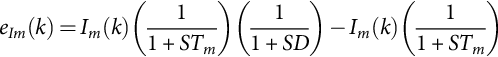
ePm(k)=Im(k)×ωm(k)(11+STm)(11+SD)−Im(k)×ωm(k)(11+STm)
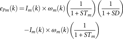
and the total or global error etm(k) for the MPFC scheme at a time instant
etm(k)=γωmeωm(k)+γimeim(k)+γpmepm(k)
A number of conflicting objective functions are selected to optimize using the PSO algorithm. These functions are defined by the following:
J1=Minimizethetotalharmonicdistortionoftheloadcurrent(THDi)
J2=Minimizethetotalharmonicdistortionoftheloadvoltage(THDv)
J3=Maximizetheelectricenergyefficiency
J4=Maximizethepowerfactor
J5=MinimizetheKWhconsumption
In general, to solve this complex optimality search problem, there are two possible optimization techniques based on particle swarm optimization (PSO): single aggregate selected objective optimization (SOO), which is explained, and multiobjective optimization (MOO). The main procedure of the SOO is based on selecting a single aggregate objective function with weighted single-objective parameters scaled by a number of weighting factors. The objective function is optimized (either minimized or maximized) using either GA or particle swarm optimization search algorithm (PSO) methods to obtain a single global or near-optimal solution. On the other hand, the main objective of the multiobjective (MO) problem is finding the set of acceptable (trade-off) optimal solutions. This set of accepted solutions is called Pareto front. These acceptable trade-off multilevel solutions give more ability to the user to make an informed decision by seeing a wide range of near-optimal selected solutions that are feasible and acceptable from an “overall” standpoint. Single-objective (SO) optimization may ignore this trade-off viewpoint, which is crucial. The main advantages of the proposed MOO method are the following: It doesn't require a priori knowledge of the relative importance of the objective functions, and it provides a set of acceptable trade-off near-optimal solutions. This set is called Pareto front or optimality trade-off surfaces. Both SOO and MOO searching algorithms are tested, validated, and compared.
The dynamic error-driven controller regulates the controllers' gains using the particle swarm optimization (PSO) and GA to minimize the system total error and the selected objective functions. The proposed dynamic triloop error-driven controller, developed by the first author, is a novel advanced regulation concept that operates as an adaptive dynamic-type multipurpose controller capable of handling sudden parametric changes, load and/or source excursions. By using the triloop error-driven controller, it is expected to have a smoother, less dynamic overshoot and fast and more robust controller when compared with those of classical control schemes.
Self tuned conventional PID controller
Fundamentally, the conventional PID controller comprises three basic control actions. They are simple to implement and they provide good performance. The tuning process of the gains of PID controllers can be complex because it is iterative: first, it is necessary to tune the “proportional” mode, then the “integral,” and then add the “derivative” mode to stabilize the overshoot, then add more “proportional,” and so on. The PID controller has the following form in the time domain as shown in Fig. 38.45:
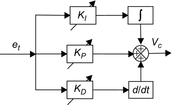
u(t)=Kpe(t)+Kit∫0e(t)dt+Kdde(t)dt
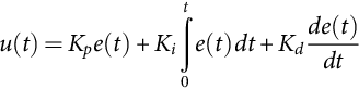
where e(t) is the selected system error, u(t) the control variable, Kp the proportional gain, Ki the integral gain, and Kd is the derivative gain. Each coefficient of the PID controller adds some special characteristics to the output response of the system. Because of this, choosing the right parameters becomes a crucial decision. In this scheme, the triloop error-driven controller is utilized with traditional PID controller. PID controller gains (KP, KI, and KD) are dynamically self-tuned using the PSO and GA dynamic search and optimization criterion based on total error minimization, steady-state error, maximum overshoot, and settling time and rising time.
38.8.3.2 Digital Simulation Results
The family of (GP-EM-EE) devices system performance is compared for two cases; with (as shown in Table 38.12) and without the (GP-EM-EE) devices, the second case is studied with fixed (as shown in Table 38.13) and self-tuned-type controllers using either GA or PSO. In addition, the second case is studied to compare the performance with artificial neural network (ANN) controller (as shown in Table 38.14) and fuzzy logic controller (FLC) (as shown in Table 38.15) with the self-tuned-type controllers using either GA or PSO. The self-tuned-type controllers based either GA or PSO is tuned conventional PID controller and has been applied to the speed tracking control of the same system parameters for performance comparison. Matlab/Simulink software was used to design, test, and validate the effectiveness of the (GP-EM-EE) devices for small motors used in household appliances, washers, dryers, fans, water pumps, ventilation systems, air conditions, and other applications in dispersing machines, actuators, and small converters with induction motor size from 5 to 25 kVA. The digital dynamic simulation model using Matlab/Simulink software environment allows for low-cost assessment and prototyping, system parameter selection, and optimization of control settings. The use of GA and PSO search algorithms is utilized in online gain adjusting to minimize controller absolute value of total error. This is required before full-scale prototyping that is both expensive and time-consuming. The effectiveness of dynamic simulators brings on detailed submodels selections and tested submodels Matlab library of power system components already tested and validated. The dynamic simulation conditions are identical for all tuned controllers. To compare the global performances of tuned conventional PID controller, the normalized mean-square-error (NMSE) deviations between output plant variables and desired values and is defined as
Table 38.12
System behavior without (GP-EM-EE) schemes
| Without (GP-EM-EE) | |
| RMS motor voltage (pu) | 0.8578 |
| RMS motor current (pu) | 0.8724 |
| Maximum transient voltage over/undershoot (pu) | 0.1797 |
| Maximum transient current—over/undershoot (pu) | 0.1875 |
| System efficiency | 0.7853 |
| NMSE_V | 0.4672 |
| NMSE_ωm | 0.6476 |
| NMSE_I | 0.4238 |
| THDv_Bus L (%) | 19.647 |
| THDi_Bus L (%) | 20.346 |
| THDv_Bus M (%) | 21.675 |
| THDi_Bus M (%) | 19.564 |
| Motor power factor | 0.7167 |
Table 38.13
System dynamic behavior comparison using the constant parameters conventional PID controller
| GP-EM-EE scheme A | GP-EM-EE scheme B | GP-EM-EE scheme C | GP-EM-EE scheme D | GP-EM-EE scheme E | |
| RMS motor voltage (pu) | 0.9762 | 0.9609 | 0.9575 | 0.9735 | 0.9690 |
| RMS Motor current (pu) | 0.7029 | 0.7008 | 0.6743 | 0.7032 | 0.6821 |
| Maximum transient voltage over/undershoot (pu) | 0.0905 | 0.0734 | 0.0729 | 0.0880 | 0.0846 |
| Maximum transient current—over/undershoot (pu) | 0.0701 | 0.0671 | 0.0884 | 0.0716 | 0.0740 |
| NMSE_V | 0.0828 | 0.0737 | 0.0781 | 0.0683 | 0.0907 |
| NMSE_ωm | 0.0809 | 0.0770 | 0.0793 | 0.0749 | 0.0773 |
| NMSE_I | 0.0722 | 0.0808 | 0.0852 | 0.0796 | 0.0823 |
| THDv_Bus L (%) | 7.8228 | 9.0412 | 8.7138 | 8.9321 | 9.5253 |
| THDi_Bus L (%) | 7.3532 | 8.3315 | 9.5150 | 7.7711 | 9.5659 |
| THDv_Bus M (%) | 8.0566 | 9.4304 | 9.1032 | 8.9371 | 9.2456 |
| THDi_Bus M (%) | 10.8589 | 8.4421 | 8.6837 | 8.3050 | 8.7230 |
| System efficiency | 0.8577 | 0.8749 | 0.9080 | 0.9186 | 0.8579 |
| Motor power factor | 0.9082 | 0.8957 | 0.8919 | 0.8721 | 0.9083 |
| Reduction in kWh consumption (%) | 14.4937 | 14.6854 | 12.2181 | 12.6337 | 12.7710 |

Table 38.14
System dynamic behavior comparison using ANN controller
| GP-EM-EE Scheme A | GP-EM-EE Scheme B | GP-EM-EE Scheme C | GP-EM-EE Scheme D | GP-EM-EE Scheme E | |
| RMS motor voltage (pu) | 0.9790 | 0.9713 | 0.9620 | 0.9723 | 0.9719 |
| RMS motor current (pu) | 0.6837 | 0.6944 | 0.6839 | 0.6887 | 0.7077 |
| Maximum transient voltage over/undershoot (pu) | 0.0769 | 0.0873 | 0.0795 | 0.0717 | 0.0830 |
| Maximum transient current—over/undershoot (pu) | 0.0871 | 0.0673 | 0.0833 | 0.0760 | 0.0869 |
| NMSE_V | 0.0790 | 0.0840 | 0.0772 | 0.0742 | 0.0714 |
| NMSE_ωm | 0.0715 | 0.0833 | 0.0741 | 0.0799 | 0.0704 |
| NMSE_I | 0.0837 | 0.0759 | 0.0876 | 0.0874 | 0.0811 |
| THDv_Bus L (%) | 10.4023 | 7.7359 | 8.6519 | 9.1624 | 9.9567 |
| THDi_Bus L (%) | 9.3573 | 8.9212 | 8.8588 | 7.4199 | 8.8514 |
| THDv_Bus M (%) | 8.5408 | 8.2842 | 10.4948 | 10.1231 | 10.8888 |
| THDi_Bus M (%) | 9.3120 | 7.1241 | 9.4659 | 10.3514 | 10.9988 |
| System efficiency | 0.8943 | 0.9163 | 0.8749 | 0.9125 | 0.8632 |
| Motor power factor | 0.8609 | 0.8715 | 0.9153 | 0.8607 | 0.8734 |
| Reduction in kWh consumption (%) | 12.3129 | 12.0158 | 14.3858 | 13.4017 | 11.8366 |
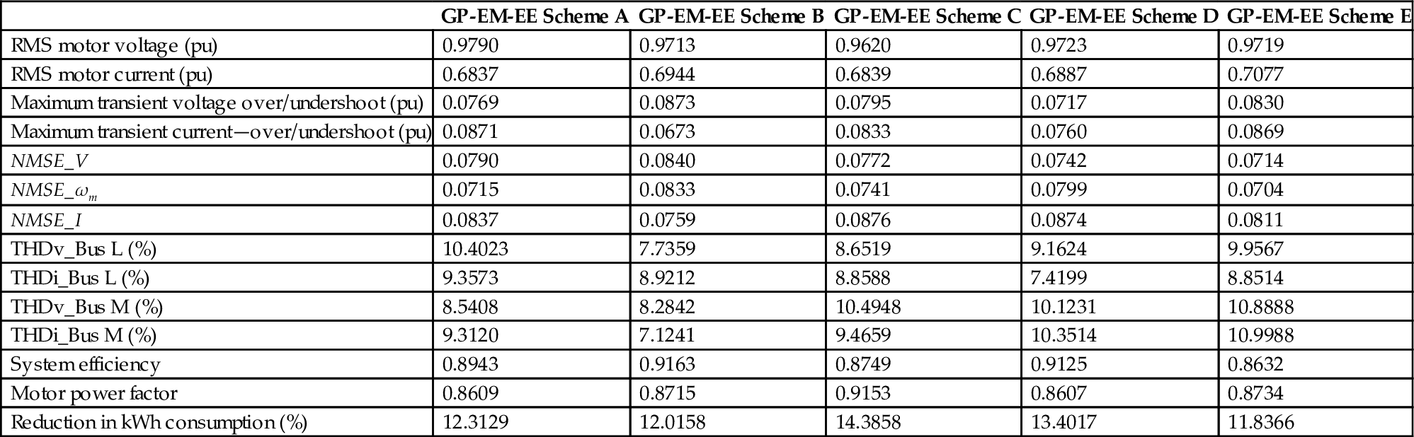
Table 38.15
System dynamic behavior comparison using the FLC controller
| GP-EM-EE scheme A | GP-EM-EE scheme B | GP-EM-EE scheme C | GP-EM-EE scheme D | GP-EM-EE scheme E | |
| RMS motor voltage (pu) | 0.9598 | 0.9573 | 0.9627 | 0.9594 | 0.9584 |
| RMS motor current (pu) | 0.6863 | 0.6893 | 0.6917 | 0.6893 | 0.6929 |
| Maximum transient voltage over/under shoot (pu) | 0.0788 | 0.0886 | 0.0867 | 0.0824 | 0.0866 |
| Maximum transient current—over/undershoot (pu) | 0.0828 | 0.0751 | 0.0738 | 0.0750 | 0.0797 |
| NMSE_V | 0.0844 | 0.0743 | 0.0871 | 0.0805 | 0.0757 |
| NMSE_ωm | 0.0838 | 0.0800 | 0.0775 | 0.0836 | 0.0818 |
| NMSE_I | 0.0860 | 0.0899 | 0.0794 | 0.0881 | 0.0710 |
| THDv_Bus L (%) | 8.2175 | 8.6528 | 9.0910 | 9.9722 | 8.2990 |
| THDi_Bus L (%) | 7.5181 | 8.8507 | 8.9451 | 7.1258 | 9.7391 |
| THDv_Bus M (%) | 9.9806 | 8.2001 | 8.1204 | 9.9178 | 10.2212 |
| THDi_Bus M (%) | 11.0353 | 8.9716 | 10.6999 | 8.8819 | 10.3043 |
| System efficiency | 0.9195 | 0.8701 | 0.8880 | 0.8750 | 0.8990 |
| Motor power factor | 0.9169 | 0.9049 | 0.8986 | 0.8650 | 0.8628 |
| Reduction in kWh consumption (%) | 11.4634 | 11.4088 | 13.0202 | 13.8055 | 12.4766 |

NMSEVS=∑(VS−VS−ref)2∑(VS−ref)2
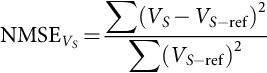
NMSEωm=∑(ωm−ωm−ref)2∑(ωm−ref)2
NMSEIs=∑(IS−IS−ref)2∑(IS−ref)2
The control system comprises the three dynamic multiloop error-driven regulator is coordinated to minimize the selected objective functions. SOO obtains a single global or near-optimal solution based on a single-weighted-objective function. The weighted single-objective function combines several objective functions using specified or selected weighting factors as follows:
weightedobjectivefunction=α1J1+α2J2+α3J3+α4J4+α5J5
where α1=0.20, α2=0.20, α3=0.20, α4=0.20, and α5=0.20 are selected weighting factors. J1, J2, J3, J4, and J5 are the selected objective functions. On the other hand, the MO finds the set of acceptable (trade-off) optimal solutions. This set of accepted solutions is called Pareto front. These acceptable trade-off multilevel solutions give more ability to the user to make an informed decision by seeing a wide range of near-optimal selected solutions. Table 38.16 shows the system behavior using traditional controllers with constant controller gains for the (GP-EM-EE) schemes. In addition, Table 38.10 shows system behavior comparison using the SOGA-based tuned conventional PID controller, and Table 38.17 shows the system behavior comparison using the MOGA-based tuned conventional PID controller. Finally, Tables 38.18 and 38.19) show system behavior comparison using the SOPSO- and MOPSO-based tuned conventional PID controller, respectively. Comparing the system dynamic response results of the two study cases, with GA and PSO tuning algorithms and traditional controllers with constant controller gain results, ANN controller and FLC, it is quite apparent that the GA and PSO tuning algorithms highly improved the system dynamic performance from a general power quality point of view. The GA and PSO tuning algorithms had a great impact on motor RMS voltage (pu) improving it from 0.8578 (without the (GP-EM-EE) device), 0.9762 (constant gains controller), 0.9790 (ANN controller), and 0.9598 (FLC) to around 0.9804 (SOGA-based tuned controller), 0.9865 (MOGA-based tuned controller), 0.9887 (SOPSO)-based tuned controller, and 0.9852 (MOPSO-based tuned controller). Motor RMS current (pu) is reduced from 0.8724 (without the (GP-EM-EE) device), 0.7029 (constant gains controller), 0.6837 (ANN controller), and 0.6863 (FLC) to around 0.6247 (SOGA-based tuned controller), 0.6304 (MOGA-based tuned controller), 0.6358 (SOPSO)-based tuned controller, and 0.6471 (MOPSO-based tuned controller). Maximum transient motor voltage over/undershoot (pu) is reduced from 0.1797 (without the (GP-EM-EE) device), 0.0905 (constant gains controller), 0.0769 (ANN controller), and 0.0788 (FLC) to around 0.0472 (SOGA-based tuned controller), 0.0394 (MOGA-based tuned controller), 0.0441 (SOPSO)-based tuned controller, and 0.0365 (MOPSO-based tuned controller). Maximum transient motor current – over/undershoot (pu) is reduced from 0.1875 (without the (GP-EM-EE) device), 0.0701 (constant gains controller), 0.0871 (ANN controller), and 0.0828 (FLC) to around 0.0431 (SOGA-based tuned controller), 0.0533 (MOGA-based tuned controller), 0.0412 (SOPSO)-based tuned controller, and 0.0563 (MOPSO-based tuned controller). Moreover, the normalized mean square error (NMSE_V) of the motor voltage is reduced from 0.4672 (without the (GP-EM-EE) device), 0.0828 (constant gains controller), 0.0790 (ANN controller), and 0.0844 (FLC) to around 0.00396 (SOGA-based tuned controller), 0.00429 (MOGA-based tuned controller), 0.00489 (SOPSO)-based tuned controller, and 0.00440 (MOPSO-based tuned controller). In addition, the (NMSE_ωm) of the SPIM motor is reduced from 0.6476 (without the (GP-EM-EE) device), 0.0809 (constant gains controller), 0.0715 (ANN controller), and 0.0838 (FLC) to around 0.00458 (SOGA-based tuned controller), 0.00608 (MOGA-based tuned controller), 0.00608 (SOPSO)-based tuned controller, and 0.00513 (MOPSO-based tuned controller). The (NMSE_I) of the motor current is reduced from 0.4238 (without the (GP-EM-EE) device), 0.0722 (constant gains controller), 0.0837 (ANN controller), and 0.0860 (FLC) to around 0.00361 (SOGA-based tuned controller), 0.00499 (MOGA-based tuned controller), 0.00602 (SOPSO)-based tuned controller, and 0.00465 (MOPSO-based tuned controller). Total harmonic distortion (THD) (%) of the supply voltage is reduced from 19.647 (without the (GP-EM-EE) device), 7.8228 (constant gains controller), 10.4023 (ANN controller), and 8.2175 (FLC) to around 6.2535 (SOGA-based tuned controller), 4.8408 (MOGA-based tuned controller), 4.2581 (SOPSO)-based tuned controller, and 4.1081 (MOPSO-based tuned controller). THD (%) of the supply current is reduced from 20.346 (without the (GP-EM-EE) device), 7.3532 (constant gains controller), 9.3573 (ANN controller), and 7.5181 (FLC) to around 4.1530 (SOGA-based tuned controller), 4.0103 (MOGA-based tuned controller), 5.2433 (SOPSO)-based tuned controller, and 5.1378 (MOPSO-based tuned controller). THD (%) of the motor voltage is reduced from 21.675 (without the (GP-EM-EE) device), 8.0566 (constant gains controller), 8.5408 (ANN controller), and 9.9806 (FLC) to around 5.7887 (SOGA-based tuned controller), 4.9313 (MOGA-based tuned controller), 4.5873 (SOPSO)-based tuned controller, and 4.3629 (MOPSO-based tuned controller). THD (%) of the motor current is reduced from 21.675 (without the (GP-EM-EE) device), 10.8589 (constant gains controller), 9.3120 (ANN controller), and 11.0353 (FLC) to around 3.9572 (SOGA-based tuned controller), 3.9998 (MOGA-based tuned controller), 5.1673 (SOPSO)-based tuned controller, and 5.1216 (MOPSO-based tuned controller). The system efficiency is improved from 0.7853 (without the (GP-EM-EE) device), 0.8577 (constant gains controller), 0.8943 (ANN controller), and 0.9195 (FLC) to around 95.4132 (SOGA-based tuned controller), 95.4882 (MOGA-based tuned controller), 95.4999 (SOPSO)-based tuned controller, and 90.7467 (MOPSO-based tuned controller). Motor power factor is improved from 0.7167 (without the (GP-EM-EE) device), 0.9082 (constant gains controller), 0.8609 (ANN controller), and 0.9169 (FLC) to around 95.1040 (SOGA-based tuned controller), 90.8137 (MOGA-based tuned controller), 91.7450 (SOPSO)-based tuned controller, and 91.4433 (MOPSO-based tuned controller). Reduction in kWh consumption (%) is reduced from 0.000 (without the (GP-EM-EE) device), 14.4937 (constant gains controller), 12.3129 (ANN controller), and 11.4634 (FLC) to around 18.3913 (SOGA-based tuned controller), 16.5388 (MOGA-based tuned controller), 15.9691 (SOPSO)-based tuned controller, and 16.5328 (MOPSO-based tuned controller).
Table 38.16
System dynamic behavior comparison using the SOGA-based tuned conventional PID controller
| GP-EM-EE scheme A | GP-EM-EE scheme B | GP-EM-EE scheme C | GP-EM-EE scheme D | GP-EM-EE scheme E | |
| RMS motor voltage (pu) | 0.9804 | 0.9810 | 0.9944 | 0.9922 | 0.9799 |
| RMS motor current (pu) | 0.6247 | 0.6237 | 0.6448 | 0.6473 | 0.6428 |
| Maximum transient voltage over/undershoot (pu) | 0.0472 | 0.0569 | 0.0565 | 0.0494 | 0.0380 |
| Maximum transient current—over/undershoot (pu) | 0.0431 | 0.0509 | 0.0403 | 0.0542 | 0.0495 |
| NMSE_V×10−1 | 0.0396 | 0.0591 | 0.0408 | 0.0359 | 0.0531 |
| NMSE_ωm×10−1 | 0.0458 | 0.0453 | 0.0585 | 0.0595 | 0.0477 |
| NMSE_I×10−1 | 0.0361 | 0.0564 | 0.0371 | 0.0380 | 0.0533 |
| THDv_Bus L (%) | 6.2535 | 5.8337 | 3.9023 | 6.1560 | 4.7221 |
| THDi_Bus L (%) | 4.1530 | 5.3045 | 6.4754 | 4.9912 | 5.3056 |
| THDv_Bus M (%) | 5.7887 | 3.6631 | 6.2107 | 6.3719 | 3.7171 |
| THDi_Bus M (%) | 3.9572 | 4.7990 | 6.6102 | 5.5482 | 5.7022 |
| System efficiency | 95.4132 | 92.3235 | 94.2164 | 95.4236 | 93.5954 |
| Motor power factor | 95.1040 | 94.4444 | 92.5749 | 94.3228 | 91.4794 |
| Reduction in kWh consumption (%) | 18.3913 | 16.2849 | 15.9924 | 18.9718 | 17.9797 |
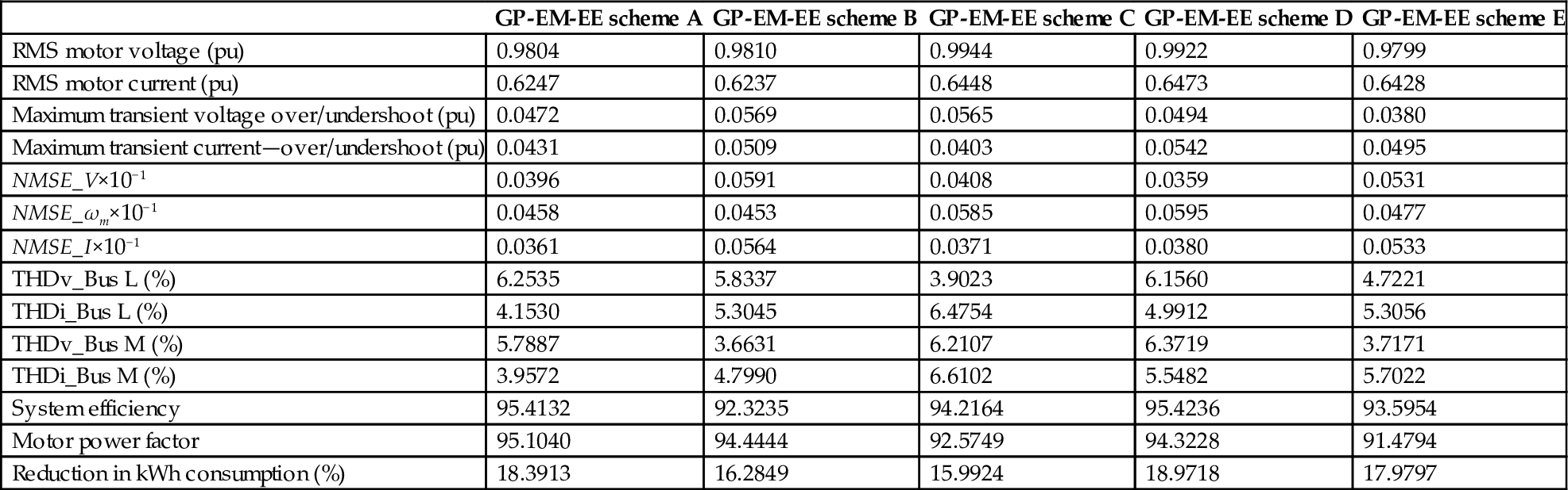
Table 38.17
System dynamic behavior comparison using a selected solution from the MOGA Pareto front-based tuned conventional PID controller
| GP-EM-EE scheme A | GP-EM-EE scheme B | GP-EM-EE scheme C | GP-EM-EE scheme D | GP-EM-EE scheme E | |
| RMS motor voltage (pu) | 0.9865 | 0.9775 | 0.9790 | 0.9767 | 0.9939 |
| RMS motor current (pu) | 0.6304 | 0.6289 | 0.6477 | 0.6338 | 0.6252 |
| Maximum transient voltage over/undershoot (pu) | 0.0394 | 0.0371 | 0.0373 | 0.0539 | 0.0365 |
| Maximum transient current—over/undershoot (pu) | 0.0533 | 0.0413 | 0.0515 | 0.0486 | 0.0502 |
| NMSE_V×10−1 | 0.0429 | 0.0582 | 0.0380 | 0.0431 | 0.0564 |
| NMSE_ωm×10−1 | 0.0608 | 0.0374 | 0.0603 | 0.0590 | 0.0599 |
| NMSE_I×10−1 | 0.0499 | 0.0597 | 0.0437 | 0.0424 | 0.0372 |
| THDv_Bus L (%) | 4.8408 | 6.6094 | 3.8605 | 4.6237 | 4.0436 |
| THDi_Bus L (%) | 4.0103 | 4.1585 | 3.9436 | 5.2812 | 5.9842 |
| THDv_Bus M (%) | 4.9313 | 6.2074 | 6.1134 | 3.6848 | 5.6249 |
| THDi_Bus M (%) | 3.9998 | 4.3153 | 6.4326 | 4.0984 | 4.2902 |
| System efficiency | 95.4882 | 91.6483 | 94.5787 | 93.7556 | 91.4767 |
| Motor power factor | 90.8137 | 92.1151 | 95.5633 | 95.4594 | 91.8090 |
| Reduction in kWh consumption (%) | 16.5388 | 16.5127 | 19.0189 | 20.4335 | 15.4505 |

Table 38.18
System dynamic behavior comparison using the SOPSO-based tuned conventional PID controller
| GP-EM-EE scheme A | GP-EM-EE scheme B | GP-EM-EE scheme C | GP-EM-EE Scheme D | GP-EM-EE scheme E | |
| RMS motor voltage (pu) | 0.9887 | 0.9831 | 0.9901 | 0.9806 | 0.9809 |
| RMS motor current (pu) | 0.6358 | 0.6449 | 0.6456 | 0.6486 | 0.6446 |
| Maximum transient voltage over/undershoot (pu) | 0.0441 | 0.0431 | 0.0458 | 0.0365 | 0.0429 |
| Maximum transient current—over/undershoot (pu) | 0.0412 | 0.0500 | 0.0577 | 0.0421 | 0.0506 |
| NMSE_V×10−1 | 0.0489 | 0.0389 | 0.0358 | 0.0439 | 0.0448 |
| NMSE_ωm×10−1 | 0.0608 | 0.0594 | 0.0466 | 0.0593 | 0.0482 |
| NMSE_I×10−1 | 0.0602 | 0.0599 | 0.0539 | 0.0521 | 0.0575 |
| THDv_Bus L (%) | 4.2581 | 5.2727 | 5.1959 | 5.1325 | 4.8095 |
| THDi_Bus L (%) | 5.2433 | 6.1471 | 4.2937 | 4.8437 | 3.7976 |
| THDv_Bus M (%) | 4.5873 | 6.1412 | 5.7390 | 6.3506 | 3.9065 |
| THDi_Bus M (%) | 5.1673 | 4.9705 | 4.7114 | 6.4459 | 4.1457 |
| System efficiency | 95.4999 | 94.0919 | 90.9345 | 93.6876 | 92.6432 |
| Motor power factor | 91.7450 | 91.5784 | 91.0446 | 90.6943 | 94.6423 |
| Reduction in kWh consumption (%) | 15.9691 | 18.6019 | 14.9762 | 16.0446 | 18.6966 |

Table 38.19
System dynamic behavior comparison using a selected solution from the MOPSO Pareto front-based tuned conventional PID controller
| GP-EM-EE Scheme A | GP-EM-EE Scheme B | GP-EM-EE Scheme C | GP-EM-EE Scheme D | GP-EM-EE Scheme E | |
| RMS motor voltage (pu) | 0.9852 | 0.9830 | 0.9816 | 0.9915 | 0.9847 |
| RMS motor current (pu) | 0.6471 | 0.6407 | 0.6249 | 0.6353 | 0.6278 |
| Maximum transient voltage over/undershoot (pu) | 0.0365 | 0.0449 | 0.0380 | 0.0441 | 0.0359 |
| Maximum transient current—over/undershoot (pu) | 0.0563 | 0.0363 | 0.0464 | 0.0365 | 0.0528 |
| NMSE_V×10−1 | 0.0440 | 0.0498 | 0.0464 | 0.0395 | 0.0373 |
| NMSE_ωm×10−1 | 0.0513 | 0.0516 | 0.0401 | 0.0460 | 0.0535 |
| NMSE_I×10−1 | 0.0465 | 0.0410 | 0.0506 | 0.0568 | 0.0581 |
| THDv_Bus L (%) | 4.1081 | 4.1093 | 5.6076 | 3.9418 | 6.4921 |
| THDi_Bus L (%) | 5.1378 | 4.1551 | 4.5004 | 4.0566 | 3.7277 |
| THDv_Bus M (%) | 4.3629 | 6.2371 | 5.8741 | 5.7775 | 4.8263 |
| THDi_Bus M (%) | 5.1216 | 6.6090 | 6.0487 | 4.9076 | 6.5793 |
| System efficiency | 90.7467 | 95.0928 | 92.4381 | 94.3056 | 95.5501 |
| Motor power factor | 91.4433 | 91.4801 | 92.2403 | 90.8052 | 92.4638 |
| Reduction in kWh consumption (%) | 16.5328 | 16.2839 | 17.9038 | 15.6451 | 15.9338 |
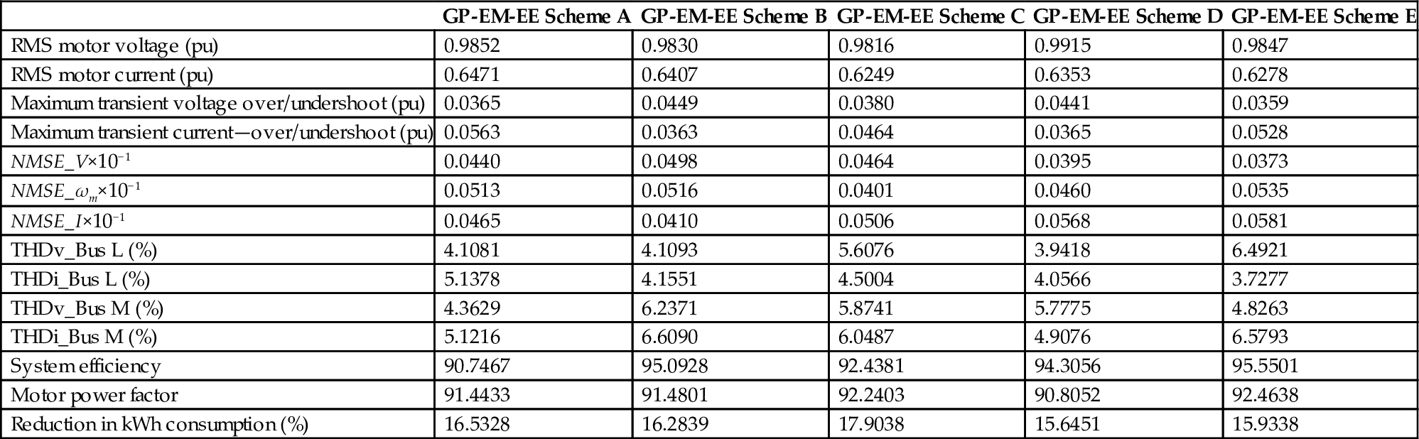
The application validated the operation of a novel wind-driven squirrel cage induction generator fed from single-phase supply. The scheme utilizes a simple but effective series-parallel switched capacitor filter to ensure dynamic terminal voltage stabilization, effective energy utilization, and minimal impact of electric load switching and dynamic excursions and wind velocity changes. The novel error-driven self-regulating multiloop dynamic controller utilizes random search optimization algorithms using particle swarm optimization (PSO) and GA to continuously search for effective and optimized controllers gains that can cope with specified objective function restrictions of minimum voltage deviations, limited generated current and power excursions due to terminal load changes, and wind velocity excursions and gusting. The application presents a family of novel low-cost green plug electricity saving devices/energy management/energy economizer (GP-EM-EE) devices equipped with a dynamic online error-driven optimally tuned controller. The (GP-EM-EE) are small low-cost energy conservation devices in the form add-on dynamic switched capacitor filter compensator schemes for low horsepower motors used in household appliances, washers, dryers, fans, water pumps, ventilation systems, air conditioners, and other cyclic motorized loads used in dispersing machines, actuators, and small converters with induction motor size from 5 to 25 kVA. The (GP-EM-EE) devices family can be used with all types of small horsepower motors with billions of small motors used in multitude of applications that consumes over 50%–60% of total electric energy generated in the world. The (GP-EM-EE) device can save 10–20% of the electricity cost of operating the small motor over the estimated motor life span of 7–10 years. This translates into millions of dollars in daily electricity savings, reduced electric utility overloading conditions, blackouts, brownouts, and enhanced, secure, and reliable operation with additional sizable power capacity release due to reduced electric demand and feeder losses.
38.9 Conclusion
The chapter covers novel techniques for the dynamic control of industrial motor drives. The use of AI soft computing PSO and GA random search techniques is presented. The specific use of PSO and GA single-objective and multiobjective controller optimization and dynamic gains adjusting is illustrated using three key applications of optimal operation of induction motor drives, hybrid photovoltaic-fuel cell-diesel-battery electric vehicle drive system, and finally, the novel self-regulating green plug-energy management energy economizer schemes developed by the first author as a number of an extended family of modulated power filters, switched capacitor compensators, and dynamic electric energy management devices and system. The control strategies are all based on multiloop error-driven regulation with online dynamic gain adjusting based on PSO and GA search algorithm. The use of AI self-regulating dynamic controllers based on AI soft computing allows meeting a multitude of conflicting objective functions of effective speed reference tracking, minimal losses, efficient utilization, limited inrush currents under parametric variations, supply source excursions, inertia, and mechanical load nonlinear loads. The other added benefit is targeting the use of power electronic devices and switched capacitor compensator/filters in ensuring efficient operation of motors and motor drives especially in future applications using renewable and green energy system.