
Dividend Discount Models
In this entry, we discuss dividend discount models and their limitations. We begin with a review of the various ways to measure dividends and then take a look at how dividends and stock prices are related.
DIVIDEND MEASURES
Dividends are measured using three different measures:
- Dividends per share
- Dividend yield
- Dividend payout
The value of a share of stock today is the investors’ assessment of today’s worth of future cash flows for each share. Because future cash flows to shareholders are dividends, we need a measure of dividends for each share of stock to estimate future cash flows per share. The dividends per share is the dollar amount of dividends paid out during the period per share of common stock:
If a company has paid $600,000 in dividends during the period and there are 1.5 million shares of common stock outstanding, then
The company paid out 40 cents in dividends per common share during this period.
The dividend yield, the ratio of dividends to price, is
The dividend yield is also referred to as the dividend-price ratio. Historically, the dividend yield for U.S. stocks has been a little less than 5%, according to a study by Campbell and Shiller (1998). In an exhaustive study of the relation between dividend yield and stock prices, Campbell and Shiller find that:
- There is a weak relation between the dividend yield and subsequent 10-year dividend growth.
- The dividend yield does not forecast future dividend growth.
- The dividend yield predicts future price changes.
The weak relation between the dividend yield and future dividends may be attributed to the effects of the business cycle on dividend growth. The tendency for the dividend yield to revert to its historical mean has been observed by researchers.
Another way of describing dividends paid out during a period is to state the dividends as a portion of earnings for the period. This is referred to as the dividend payout ratio:
If a company pays $360,000 in dividends and has earnings available to common shareholders of $1.2 million, the payout ratio is 30%:
This means that the company paid out 30% of its earnings to shareholders.
The proportion of earnings paid out in dividends varies by company and industry. For example, the companies in the steel industry typically pay out 25% of their earnings in dividends, whereas the electric utility companies pay out approximately 75% of their earnings in dividends.
If companies focus on dividends per share in establishing their dividends (e.g., a constant dividends per share), the dividend payout will fluctuate along with earnings. We generally observe that companies set the dividend policy such that dividends per share grow at a relatively constant rate, resulting in dividend payouts that fluctuate.
DIVIDENDS AND STOCK PRICES
If an investor buys a common stock, he or she has bought shares that represent an ownership interest in the corporation. Shares of common perpetual security—there is no maturity. The investor who owns shares of common stock has the right to receive a certain portion of any dividends—but dividends are not a sure thing. Whether or not a corporation pays dividends is up to its board of directors—the representatives of the common shareholders. Typically, we see some pattern in the dividends companies pay: Dividends are either constant or grow at a constant rate. But there is no guarantee that dividends will be paid in the future.
Preferred shareholders are in a similar situation as the common shareholders. They expect to receive cash dividends in the future, but the payment of these dividends is up to the board of directors. But there are three major differences between the dividends of preferred and common shares. First, the dividends on preferred stock usually are specified at a fixed rate or dollar amount, whereas the amount of dividends is not specified for common shares. Second, preferred shareholders are given preference: their dividends must be paid before any dividends are paid on common stock. Third, if the preferred stock has a cumulative feature, dividends not paid in one period accumulate and are carried over to the next period. Therefore, the dividends on preferred stock are more certain than those on common shares.
It is reasonable to figure that what an investor pays for a share of stock should reflect what he or she expects to receive from it—return on the investor’s investment. What an investor receives are cash dividends in the future. How can we relate that return to what a share of common stock is worth? Well, the value of a share of stock should be equal to the present value of all the future cash flows an investor expects to receive from that share. To value stock, therefore, an investor must project future cash flows, which, in turn, means projecting future dividends. This approach to the valuation of common stock is referred to as the discounted cash flow approach and the models used are referred to as dividend discount models.
Dividend discount models are not the only approach to valuing common stock. There are fundamental factor models, also referred to as multifactor equity models.
BASIC DIVIDEND DISCOUNT MODELS
As discussed above, the basis for the dividend discount model (DDM) is simply the application of present value analysis, which asserts that the fair price of an asset is the present value of the expected cash flows. This model was first suggested by Williams (1938). In the case of common stock, the cash flows are the expected dividend payouts. The basic DDM model can be expressed mathematically as:
where
The dividends are expected to be received forever.
Practitioners rarely use the dividend discount model given by equation (1). Instead, one of the DDMs discussed below is typically used.
THE FINITE LIFE GENERAL DIVIDEND DISCOUNT MODEL
The DDM given by equation (1) can be modified by assuming a finite life for the expected cash flows. In this case, the expected cash flows are the expected dividend payouts and the expected sale price of the stock at some future date. The expected sale price is also called the terminal price and is intended to capture the future value of all subsequent dividend payouts. This model is called the finite life general DDM and is expressed mathematically as:
where
and P, Dt, and rt are the same as defined above.
Assuming a Constant Discount Rate
A special case of the finite life general DDM that is more commonly used in practice is one in which it is assumed that the discount rate is constant. That is, it is assumed each rt is the same for all t. Denoting this constant discount rate by r, equation (2) becomes:
Equation (3) is called the constant discount rate version of the finite life general DDM. When practitioners use any of the DDM models presented in this entry, typically the constant discount rate version form is used.
Let’s illustrate the finite life general DDM assuming a constant discount rate assuming each period is a year. Suppose that the following data are determined for stock XYZ by a financial analyst:
Based on these data, the fair price of stock XYZ is
Required Inputs
The finite life general DDM requires three forecasts as inputs to calculate the fair value of a stock:
Thus the relevant question is, How accurately can these inputs be forecasted?
The terminal price is the most difficult of the three forecasts. According to theory, PN is the present value of all future dividends after N; that is, DN+1, DN+2, … , Dinfinity. Also, the future discount rate (rt) must be forecasted. In practice, forecasts are made of either dividends (DN) or earnings (EN) first, and then the price PN is estimated by assigning an “appropriate” requirement for yield, price-earnings ratio, or capitalization rate. Note that the present value of the expected terminal price PN/(1 + r)N becomes very small if N is very large.
The forecasting of dividends is “somewhat” easier. Usually, past history is available, management can be queried, and cash flows can be projected for a given scenario. The discount rate r is the required rate of return. Forecasting r is more complex than forecasting dividends, although not nearly as difficult as forecasting the terminal price (which requires a forecast of future discount rates as well). As noted above, in practice for a given company r is assumed to be constant for all periods and typically generated from the capital asset pricing model (CAPM). The CAPM provides the expected return for a company based on its systematic risk (beta).
Assessing Fair Value
Given the fair price derived from a dividend discount model, the assessment of the stock proceeds along the following lines. If the market price is below the fair price derived from the model, the stock is undervalued or cheap. The opposite holds for a stock whose market price is greater than the model-derived price. In this case, the stock is said to be overvalued or expensive. A stock trading equal to or close to its fair price is said to be fairly valued.
The DDM tells us the fair price but does not tell us when the price of the stock should be expected to move to this fair price. That is, the model says that based on the inputs generated by the analyst, the stock may be cheap, expensive, or priced appropriately. However, it does not tell us that if it is mispriced how long it will take before the market recognizes the mispricing and corrects it. As a result, an investor may hold on to a stock perceived to be cheap for an extended period of time and may underperform a benchmark during that period.
While a stock may be mispriced, an investor must also consider how mispriced it is in order to take the appropriate action (buy a cheap stock and sell or sell short an expensive stock). This will depend on the degree of mispricing and transaction costs.
CONSTANT GROWTH DIVIDEND DISCOUNT MODEL
If future dividends are assumed to grow at a constant rate (g) and a single discount rate (r) is used, then the finite life general DDM assuming a constant growth rate given by equation (3) becomes
and it can be shown that if N is assumed to approach infinity, equation (4) is equal to:
Equation (5) is the constant growth dividend discount model (Gordon and Shapiro, 1956). An equivalent formulation for the constant growth DDM is
(6) ![]()
where D1 is equal to D0(1 + g).
Consider a company that currently pays dividends of $3.00 per share. If the dividend is expected to grow at a rate of 3% per year and the discount rate is 12%, what is the value of a share of stock of this company? Using equation (5),
![]()
If the growth rate for this company’s dividends is 5%, instead of 3%, the current value is $45.00:
![]()
Therefore, the greater the expected growth rate of dividends, the greater the value of a share of stock.
In this last example, if the discount rate is 14% instead of 12% and the growth rate of dividends is 3%, the value of a share of stock is:
![]()
Therefore, the greater the discount rate, the lower the current value of a share of stock.
Let’s apply the model as given by equation (5) to estimate the price of three companies: Eli Lilly, Schering-Plough, and Wyeth Laboratories. The discount rate for each company was estimated using the capital asset pricing model assuming (1) a market risk premium of 5% and (2) a risk-free rate of 4.63%. The market risk premium is based on the historical spread between the return on the market (often proxied with the return on the S&P 500 Index) and the risk-free rate. Historically, this spread has been approximately 5%. The risk-free rate is often estimated by the yield on U.S. Treasury securities. At the end of 2006, 10-year Treasury securities were yielding approximately 4.625%. We use 4.63% as an estimate for the purposes of this illustration. The beta estimate for each company was obtained from the Value Line Investment Survey: 0.9 for Eli Lilly, 1.0 for Schering-Plough and Wyeth. The discount rate, r, for each company based on the CAPM is:
| Eli Lilly | r = 0.0463 + 0.9 (0.05) = 9.125% |
| Schering-Plough | r = 0.0463 + 1.0 (0.05) = 9.625% |
| Wyeth | r = 0.0463 + 1.0 (0.05) = 9.625% |
The dividend growth rate can be estimated by using the compounded rate of growth of historical dividends.
The compound growth rate, g, is found using the following formula:
![]()
This formula is equivalent to calculating the geometric mean of 1 plus the percentage change over the number of years. Using time value of money math, the 2006 dividend is the future value, the starting dividend is the present value, the number of years is the number of periods; solving for the interest rate produces the growth rate.
Substituting the values for the starting and ending dividend amounts and the number of periods into the formula, we get:
The value of D0, the estimate for g, and the discount rate r for each company are summarized below:

Substituting these values into equation (5), we obtain:
Schering-Plough estimated price
Comparing the estimated price with the actual price, we see that this model does not do a good job of pricing these stocks:
| Estimated | Actual price | |
| price at the | at the end | |
| Company | end of 2006 | of 2006 |
| Eli Lilly | $162.80 | $49.87 |
| Schering-Plough | $3.00 | $23.44 |
| Wyeth | $17.16 | $50.52 |
Notice that the constant growth DDM is considerably off the mark for all three companies. The reasons include: (1) the dividend growth pattern for none of the three companies appears to suggest a constant growth rate, and (2) the growth rate of dividends in recent years has been much slower than earlier years (and, in fact, negative for Schering-Plough after 2003), causing growth rates estimated from the long time periods to overstate future growth. And this pattern is not unique to these companies.
Another problem that arises in using the constant growth rate model is that the growth rate of dividends may exceed the discount rate, r. Consider the following three companies and their dividend growth over the 16-year period from 1991 through 2006, with the estimated required rates of return:
For these three companies, the growth rate of dividends over the prior 16 years is greater than the discount rate. If we substitute the D0 (the 2006 dividends), the g, and the r into equation (5), the estimated price at the end of 2006 is negative, which doesn’t make sense. Therefore, there are some cases in which it is inappropriate to use the constant rate DDM.
The potential for misvaluation using the constant rate DDM is highlighted by Fogler (1988) in his illustration using ABC prior to its being taken over by Capital Cities in 1985. He estimated the value of ABC stock to be $53.88, which was less than its market price at the time (of $64) and less than the $121 paid per share by Capital Cities.
MULTIPHASE DIVIDEND DISCOUNT MODELS
The assumption of constant growth is unrealistic and can even be misleading. Instead, most practitioners modify the constant growth DDM by assuming that companies will go through different growth phases. Within a given phase, dividends are assumed to grow at a constant rate. Molodovsky, May, and Chattiner (1965) were some of the pioneers in modifying the DDM to accommodate different growth rates.
Two-Stage Growth Model
The simplest form of multi-phase DDM is the two-stage growth model. A simple extension of equation (4) uses two different values of g. Referring to the first growth rate as g1 and the second growth rate as g2 and assuming that the first growth rate pertains to the next four years and the second growth rate refers to all years following, equation (4) can be modified as:

which simplifies to:
Because dividends following the fourth year are presumed to grow at a constant rate g2 forever, the value of a share at the end of the fourth year (that is, P4) is determined by using equation (5), substituting D0(1 + g1)4 for D0 (because period 4 is the base period for the value at end of the fourth year) and g2 for the constant rate g:
(7) 
Suppose a company’s dividends are expected to grow at 4% rate for the next four years and then 8% thereafter. If the current dividend is $2.00 and the discount rate is 12%,
If this company’s dividends are expected to grow at the rate of 4% forever, the value of a share is $26.00; if this company’s dividends are expected to grow at the rate of 8% forever, the value of a share is $52.00. But because the growth rate of dividends is expected to increase from 4% to 8% in four years, the value of a share is between those two values, or $46.87.
As you can see from this example, the basic valuation model can be modified to accommodate different patterns of expected dividend growth.
Three-Stage Growth Model
The most popular multiphase model employed by practitioners appears to be the three-stage DDM. (The formula for this model is derived in Sorensen and Williamson [1985].) This model assumes that all companies go through three phases, analogous to the concept of the product life cycle. In the growth phase, a company experiences rapid earnings growth as it produces new products and expands market share. In the transition phase the company’s earnings begin to mature and decelerate to the rate of growth of the economy as a whole. At this point, the company is in the maturity phase in which earnings continue to grow at the rate of the general economy.
Different companies are assumed to be at different phases in the three-phase model. An emerging growth company would have a longer growth phase than a more mature company. Some companies are considered to have higher initial growth rates and hence longer growth and transition phases. Other companies may be considered to have lower current growth rates and hence shorter growth and transition phases.
In the typical investment management organization, analysts supply the projected earnings, dividends, growth rates for earnings, and dividend and payout ratios using fundamental security analysis. The growth rate at maturity for the entire economy is applied to all companies. As a generalization, approximately 25% of the expected return from a company (projected by the DDM) comes from the growth phase, 25% from the transition phase, and 50% from the maturity phase. However, a company with high growth and low dividend payouts shifts the relative contribution toward the maturity phase, while a company with low growth and a high payout shifts the relative contribution toward the growth and transition phases.
STOCHASTIC DIVIDEND DISCOUNT MODELS
As we noted in our discussion and illustration of the constant growth DDM, an erratic dividend pattern such as that of Wyeth can lead to quite a difference between the estimated price and the actual price. In the case of the pharmaceutical companies, the estimated price overstated the actual price for Eli Lilly, but understated the price of Schering-Plough and Wyeth.
Hurley and Johnson (1998a, 1998b) have suggested a new family of valuation model. Their model allows for a more realistic pattern of dividend payments. The basic model generates dividend payments based on a model that assumes that either the firm will increase dividends for the period by a constant amount or keep dividends the same. The model is referred to as a stochastic DDM because the dividend can increase or be constant based on some estimated probability of each possibility occurring. The dividend stream used in the stochastic DDM is called the stochastic dividend stream.
There are two versions of the stochastic DDM. One assumes that dividends either increase or decrease at a constant growth rate. This version is referred to as a binomial stochastic DDM because there are two possibilities for dividends. The second version is called a trinomial stochastic DDM because it allows for an increase in dividends, no change in dividends, and a cut in dividends. We discuss each version below.
Binomial Stochastic Model
For both the binomial and trinomial stochastic DDM, there are two versions of the model—the additive growth model and the geometric growth model. The former model assumes that dividend growth is additive rather than geometric. This means that dividends are assumed to grow by a constant dollar amount. So, for example, if dividends are $2.00 today and the additive growth rate is assumed to be $0.25 per year, then next year dividends will grow to $2.25, in two years dividends will grow to $2.50, and so on. The second model assumes a geometric rate of dividend growth. This is the same growth rate assumption used in the earlier DDMs presented in this entry.
Binomial Additive Stochastic Model
This formulation of the model is expressed as follows:
![]()
where
Hurley and Johnson (1998a) have shown that the theoretical value of the stock based on the additive stochastic DDM assuming a constant discount rate is equal to:
For example, consider once again Wyeth. In the illustration of the constant growth model, we used D0 of $1.01 and a g of 3.533%. We estimate C by calculating the dollar increase in dividends for each year that had a dividend increase and then taking the average dollar dividend increase. The average of the increases is $0.0373.
In the 15-year span 1991 through 2006, dividends increased 11 of the 14 year-to-year differences. Therefore, p = 11/15 = 73.3333%. Substituting these values into equation (8), we find the estimated price to be:
Applying this model to the other two pharmaceutical companies, we see that the model produces an estimated price that is closer to the actual price than the fair value based on the constant growth model:
Binomial Geometric Stochastic Model
Letting g be the growth rate of dividends, then the geometric dividend stream is
![]()
Hurley and Johnson (1998b) show that the price of the stock in this case is:
Equation (9) is the binomial stochastic DDM assuming a geometric growth rate and a constant discount rate.
Trinomial Stochastic Models
The trinomial stochastic DDM allows for dividend cuts. Within the Hurley-Johnson stochastic DDM framework, Yao (1997) derived this model that allows for a cut in dividends. He notes that is not uncommon for a firm to cut dividends temporarily. In fact, an examination of the dividend record of the electric utilities industry as published in Value Line Industry Review found that in the aggregate firms cut dividends three times over a 15-year period.
Table 1 Fit of the Different Dividend Models Applied to Five Electric Utilities
Trinomial Additive Stochastic Model
The additive stochastic DDM can be extended to allow for dividend cuts as follow:
where
The theoretical value of the stock based on the trinomial additive stochastic DDM then becomes:
Notice that when pD is zero (that is, there is no possibility for a cut in dividends), equation (10) reduces to equation (8).
Trinomial Geometric Stochastic Model
For the trinomial geometric stochastic DDM allowing for a possibility of cuts, we have:

and the theoretical price is:
Once again, substituting zero for pD, equation (11) reduces to equation (9)—the binomial geometric stochastic DDM.
Applications of the Stochastic DDM
Yao (1997) applied the stochastic DDMs to five electric utility stocks that had regular dividends from 1979 to 1994 and found that the models fit the various utility stocks differently.
We see similar results in an updated example using five electric utilities, as shown in Table 1. For three of the five utilities, the binomial model provides an estimate closest to the actual stock price, whereas for the other two utilities, the trinomial model offers the closest estimate. In none of the cases, however, did the constant dividend growth model offer the closest approximation to the actual stock price.
Advantages of the Stochastic DDM
The stochatic DDM developed by Hurley and Johnson is a powerful tool for the analyst because it allows the analyst to generate a probability distribution for a stock’s value. The probability distribution can be used by an analyst to assess whether a stock is sufficiently mispriced to justify a buy or sell recommendation. For example, suppose that a three-phase DDM indicates that the value of a stock trading at $35 is $42. According to the model, the stock is underpriced and the analyst would recommend the purchase of this stock. However, the analyst cannot express his or her confidence as to the degree to which the stock is undervalued.
Hurley and Johnson show how the stochastic DDM can be used to overcome this limitation of traditional DDMs. An analyst can use the derived probability distribution from the stochastic DDM to assess the probability that the stock is undervalued. For example, an analyst may find from a probability distribution that the probability that the stock is greater than $35 (the market price) is 90%.
To employ a stochastic DDM an analyst must be prepared to make subjective assumptions about the uncertain nature of future dividends. Monte Carlo simulation available on a spread sheet (@RISK in Excel, for example) can then be used to generate the probability distribution.
EXPECTED RETURNS AND DIVIDEND DISCOUNT MODELS
Thus far, we have seen how to calculate the fair price of a stock given the estimates of dividends, discount rates, terminal prices, and growth rates. The model-derived price is then compared to the actual price and the appropriate action is taken.
The analysis can be recast in terms of expected return. This is found by calculating the return that will make the present value of the expected cash flows equal to the actual price. Mathematically, this is expressed as follows:
where
The expected return (ER) in equation (12). For example, consider the following inputs used at the outset of this entry to illustrate the finite life general DDM as given by equation (3). For stock XYZ, the inputs assumed are:
![]()
We calculated a fair price based on equation (3) to be $24.90. Suppose that the actual price is $25.89. Then the expected return is found by solving the following equation for ER:
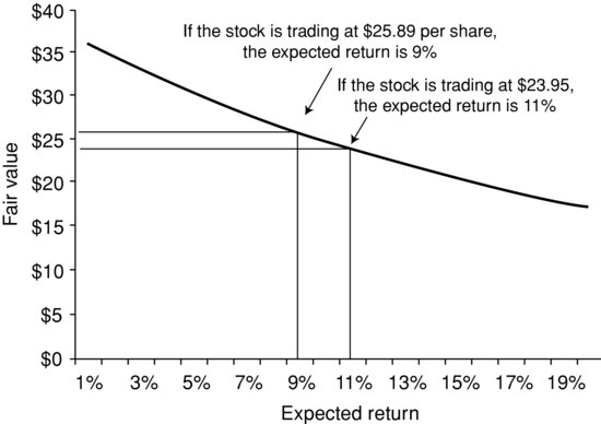
Figure 1 The Relation between the Fair Value of a Stock and the Stock’s Expected Return

The expected return is 9%.
The expected return is the discount rate that equates the present value of the expected future cash flows with the present value of the stock. The higher the expected return—for a given set of future cash flows—the lower the current value. The relation between the fair value of a stock and the expected return of a stock is shown in Figure 1.
Given the expected return and the required return (that is, the value for r), any mispricing can be identified. If the expected return exceeds the required return, then the stock is undervalued; if it is less than the required return then the stock is overvalued. A stock is fairly valued if the expected return is equal to the required return. In our illustration, the expected return (9%) is less than the required return (10%); therefore, stock XYZ is overvalued.
With the same set of inputs, the identification of a stock being mispriced or fairly valued will be the same regardless of whether the fair value is determined and compared to the market price or the expected return is calculated and compared to the required return. In the case of XYZ stock, the fair value is $24.90. If the stock is trading at $25.89, it is overvalued. The expected return if the stock is trading at $25.89 is 9%, which is less than the required return of 10%. If, instead, the stock price is $24.90, it is fairly valued. The expected return can be shown to be 10%, which is the same as the required return. At a price of $23.95, it can be shown that the expected return is 11%. Since the required return is 10%, stock XYZ would be undervalued.
While the illustration above uses the basic DDM, the expected return can be computed for any of the models. In some cases, the calculation of the expected return is simple since a formula can be derived that specifies the expected return in terms of the other variables. For example, for the constant growth DDM given by equation (5), the expected return (r) can be easily solved to give:
![]()
Rearranging the constant growth model to solve for the expected return, we see that the required rate of return can be specified as the sum of the dividend yield and the expected growth rate of dividends.
KEY POINTS
- Dividends are measured in a number of ways, including dividends per share, dividend yield, and dividend payout.
- The discounted cash flow approach to valuing common stock requires projecting future dividends. Hence, the model used to value common stock is called a dividend discount model.
- The simplest dividend discount model is the constant growth model. More complex models include the multiphase model and stochastic models.
- Stock valuation using a dividend discount model is highly dependent on the inputs used.
- A dividend discount model does not indicate when the current market price will reach its fair value.
- The output of a dividend discount model is the fair price. However, the model can be used to generate the expected return.
- The expected return is the interest rate that will make the present value of the expected dividends plus terminal price equal to the stock’s market price. The expected return is then compared to the required return to assess whether a stock is fairly priced in the market.
REFERENCES
Campbell, J. Y., and Shiller, R. J. (1998). Valuation ratios and the long-run stock market outlook. Journal of Portfolio Management 24 (Winter): 11–26.
Fogler, R. H. (1988). Security analysis, DDMs, and probability. In Equity Markets and Valuation Methods (pp. 51–52). Charlottesville, VA: The Institute of Chartered Financial Analysts.
Gordon, M., and Shapiro, E. (1956). Capital equipment analysis: The required rate of profit. Management Science 3: 102–110.
Hurley, W. J., and Johnson, L. (1994). A realistic dividend valuation model. Financial Analysts Journal 50 (July–August): 50–54.
Hurley, W. J., and Johnson, L. (1998a). Generalized Markov dividend discount models. Journal of Portfolio Management 25 (Fall): 27–31.
Hurley, W. J., and Johnson, L. (1998b). The Theory and Application of Stochastic Dividend Models. Monograph 7, Clarica Financial Services Research Centre, School of Business and Economics, Wilfrid Laurier University.
Molodovsky, N., May, C., and Chattiner, S. (1965). Common stock valuation: Principles, tables, and applications. Financial Analysts Journal 21 (November--December): 111–117.
Sorensen, E., and Williamson, E. (1985). Some evidence on the value of dividend discount models. Financial Analysts Journal 41 (November–December): 60–69.
Williams, J. B. (1938). The Theory of Investment Value. Cambridge, MA: Harvard University Press.
Yao, Y. (1997). A trinomial dividend valuation model. Journal of Portfolio Management 21 (Summer): 99–103.