
Financial Ratio Analysis
Financial analysis is one of the many tools useful in valuation because it helps analysts and investors gauge returns and risks. In this entry, we explain and illustrate financial ratios—one of the tools of financial analysis. In financial ratio analysis we select the relevant information—primarily the financial statement data—and evaluate it. We show how to incorporate market data and economic data in the analysis of financial ratios. Finally, we show how to interpret financial ratio analysis, identifying the pitfalls that occur when it’s not done properly.
RATIOS AND THEIR CLASSIFICATION
A ratio is a mathematical relation between two quantities. Suppose you have 200 apples and 100 oranges. The ratio of apples to oranges is 200/100, which we can conveniently express as 2:1 or 2. A financial ratio is a comparison between one bit of financial information and another. Consider the ratio of current assets to current liabilities, which we refer to as the current ratio. This ratio is a comparison between assets that can be readily turned into cash—current assets—and the obligations that are due in the near future—current liabilities. A current ratio of 2 or 2:1 means that we have twice as much in current assets as we need to satisfy obligations due in the near future.
Ratios can be classified according to the way they are constructed and the financial characteristic they are describing. For example, we will see that the current ratio is constructed as a coverage ratio (the ratio of current assets—available funds—to current liabilities—the obligation) that we use to describe a firm’s liquidity (its ability to meet its immediate needs).
There are as many different financial ratios as there are possible combinations of items appearing on the income statement, balance sheet, and statement of cash flows. We can classify ratios according to how they are constructed or according to the financial characteristic that they capture.
Ratios can be constructed in the following four ways:
In addition, we can also express financial data in terms of time—say, how many days’ worth of inventory we have on hand—or on a per-share basis—say, how much a firm has earned for each share of common stock. Both are measures we can use to evaluate operating performance or financial condition.
Table 1 Fictitious Corporation Balance Sheets for Years Ending December 31, in Thousands
| Current | Prior | |
| Year | Year | |
| ASSETS | ||
| Cash | $400 | $200 |
| Marketable securities | 200 | 0 |
| Accounts receivable | 600 | 800 |
| Inventories | 1,800 | 1,000 |
| Total current assets | $3,000 | $2,000 |
| Gross plant and equipment | $11,000 | $10,000 |
| Accumulated depreciation | (4,000) | (3,000) |
| Net plant and equipment | 7,000 | 7,000 |
| Intangible assets | 1,000 | 1,000 |
| Total assets | $11,000 | $10,000 |
| LIABILITIES AND SHAREHOLDERS’ EQUITY | ||
| Accounts payable | $500 | $400 |
| Other current liabilities | 500 | 200 |
| Long-term debt | 4,000 | 5,000 |
| Total liabilities | $5,000 | $5,600 |
| Common stock, $1 par value; | ||
| Authorized 2,000,000 shares | ||
| Issued 1,500,000 and 1,200,000 shares | 1,500 | 1,200 |
| Additional paid-in capital | 1,500 | 800 |
| Retained earnings | 3,000 | 2,400 |
| Total shareholders’ equity | 6,000 | 4,400 |
| Total liabilities and shareholders’ equity | $11,000 | $10,000 |
When we assess a firm’s operating performance, a concern is whether the company is applying its assets in an efficient and profitable manner. When an analyst assesses a firm’s financial condition, a concern is whether the company is able to meet its financial obligations. The analyst can use financial ratios to evaluate five aspects of operating performance and financial condition:
There are several ratios reflecting each of the five aspects of a firm’s operating performance and financial condition. We apply these ratios to the Fictitious Corporation, whose balance sheets, income statements, and statement of cash flows for two years are shown in Tables 1, 2, and 3, respectively. We refer to the most recent fiscal year for which financial statements are available as the “current year.” The “prior year” is the fiscal year prior to the current year.
Table 2 Fictitious Corporation Income Statements for Years Ending December 31, in Thousands
| Current | Prior | |
| Year | Year | |
| Sales | $10,000 | $9,000 |
| Cost of goods sold | (6,500) | (6,000) |
| Gross profit | $3,500 | $3,000 |
| Lease expense | (1,000) | (500) |
| Administrative expense | (500) | (500) |
| Earnings before interest and taxes (EBIT) | $2,000 | $2,000 |
| Interest | (400) | (500) |
| Earnings before taxes | $1,600 | $1,500 |
| Taxes | (400) | (500) |
| Net income | $1,200 | $1,000 |
| Preferred dividends | (100) | (100) |
| Earnings available to common shareholders | $1,100 | $900 |
| Common dividends | (500) | (400) |
| Retained earnings | $600 | $500 |
Table 3 Fictitious Company Statement of Cash Flows, Years Ended December 31, in Thousands
| Current | Prior | |
| Year | Year | |
| Cash flow from (used for) operating activities | ||
| Net income | $1,200 | $1,000 |
| Add or deduct adjustments to cash basis: | ||
| Change in accounts receivables | $200 | $(200) |
| Change in accounts payable | 100 | 400 |
| Change in marketable securities | (200) | 200 |
| Change in inventories | (800) | (600) |
| Change in other current liabilities | 300 | 0 |
| Depreciation | 1,000 | 1,000 |
| 600 | 800 | |
| Cash flow from operations | $1,800 | $1,800 |
| Cash flow from (used for) investing activities | ||
| Purchase of plant and equipment | $(1,000) | $0 |
| Cash flow from (used for) investing activities | $(1,000) | $0 |
| Cash flow from (used for) financing activities | ||
| Sale of common stock | $1,000 | $0 |
| Repayment of long-term debt | (1,000) | (1,500) |
| Payment of preferred dividends | (100) | (100) |
| Payment of common dividends | (500) | (400) |
| Cash flow from (used for) financing activities | (600) | (1,900) |
| Increase (decrease) in cash flow | $200 | $(100) |
| Cash at the beginning of the year | 200 | 300 |
| Cash at the end of the year | $400 | $200 |
The ratios we introduce here are by no means the only ones that can be formed using financial data, though they are some of the more commonly used. After becoming comfortable with the tools of financial analysis, an analyst will be able to create ratios that serve a particular evaluation objective.
RETURN-ON-INVESTMENT RATIOS
Return-on-investment ratios compare measures of benefits, such as earnings or net income, with measures of investment. For example, if an analyst wants to evaluate how well the firm uses its assets in its operations, he could calculate the return on assets—sometimes called the basic earning power ratio—as the ratio of earnings before interest and taxes (EBIT) (also known as operating earnings) to total assets:
For Fictitious Corporation, for the current year:
For every dollar invested in assets, Fictitious earned about 18 cents in the current year. This measure deals with earnings from operations; it does not consider how these operations are financed.
Another return-on-assets ratio uses net income—operating earnings less interest and taxes—instead of earnings before interest and taxes:
![]()
(In actual application the same term, return on assets, is often used to describe both ratios. It is only in the actual context or through an examination of the numbers themselves that we know which return ratio is presented. We use two different terms to describe these two return-on-asset ratios in this entry simply to avoid any confusion.)
For Fictitious in the current year:
Thus, without taking into consideration how assets are financed, the return on assets for Fictitious is 18%. Taking into consideration how assets are financed, the return on assets is 11%. The difference is due to Fictitious financing part of its total assets with debt, incurring interest of $400,000 in the current year; hence, the return-on-assets ratio excludes taxes of $400,000 in the current year from earnings in the numerator.
If we look at Fictitious’s liabilities and equities, we see that the assets are financed in part by liabilities ($1 million short term, $4 million long term) and in part by equity ($800,000 preferred stock, $5.2 million common stock). Investors may not be interested in the return the firm gets from its total investment (debt plus equity), but rather shareholders are interested in the return the firm can generate on their investment. The return on equity is the ratio of the net income shareholders receive to their equity in the stock:
For Fictitious Corporation, there is only one type of shareholder: common. For the current year:
Recap: Return-on-Investment Ratios
The return-on-investment ratios for Fictitious Corporation for the current year are:
Basic earning power = 18.18%
Return on assets = 10.91%
Return on equity = 20.00%
These return-on-investment ratios indicate:
- Fictitious earns over 18% from operations, or about 11% overall, from its assets.
- Shareholders earn 20% from their investment (measured in book value terms).
These ratios do not provide information on:
- Whether this return is due to the profit margins (that is, due to costs and revenues) or to how efficiently Fictitious uses its assets.
- The return shareholders earn on their actual investment in the firm, that is, what shareholders earn relative to their actual investment, not the book value of their investment. For example, $100 may be invested in the stock, but its value according to the balance sheet may be greater than or, more likely, less than $100.
DuPont System
The returns on investment ratios provides a “bottom line” on the performance of a company, but do not tell us anything about the “why” behind this performance. For an understanding of the “why,” an analyst must dig a bit deeper into the financial statements. A method that is useful in examining the source of performance is the DuPont system. The DuPont system is a method of breaking down return ratios into their components to determine which areas are responsible for a firm’s performance. To see how it is used, let us take a closer look at the first definition of the return on assets:
Suppose the return on assets changes from 20% in one period to 10% the next period. We do not know whether this decreased return is due to a less efficient use of the firm’s assets—that is, lower activity—or to less effective management of expenses (that is, lower profit margins). A lower return on assets could be due to lower activity, lower margins, or both. Because an analyst is interested in evaluating past operating performance to evaluate different aspects of the management of the firm and to predict future performance, knowing the source of these returns is valuable.
Let us take a closer look at the return on assets and break it down into its components: measures of activity and profit margin. We do this by relating both the numerator and the denominator to sales activity. Divide both the numerator and the denominator of the basic earning power by revenues:
which is equivalent to:
This says that the earning power of the company is related to profitability (in this case, operating profit) and a measure of activity (total asset turnover).
When analyzing a change in the company’s basic earning power, an analyst could look at this breakdown to see the change in its components: operating profit margin and total asset turnover.
This method of analyzing return ratios in terms of profit margin and turnover ratios, referred to as the DuPont System, is credited to the E.I. DuPont Corporation, whose management developed a system of breaking down return ratios into their components.
Let’s look at the return on assets of Fictitious for the two years. Its returns on assets were 20% in the prior year and 18.18% in the current year. We can decompose the firm’s returns on assets for the two years to obtain:
We see that operating profit margin declined over the two years, yet asset turnover improved slightly, from 0.9000 to 0.9091. Therefore, the return-on-assets decline is attributable to lower profit margins.
The return on assets can be broken down into its components in a similar manner:
or
![]()
The basic earning power ratio relates to the return on assets. Recognizing that:
![]()
then
The ratio of earnings before taxes to earnings before interest and taxes reflects the interest burden of the company, whereas the term (1 − tax rate) reflects the company’s tax burden. Therefore,
or
The breakdown of a return-on-equity ratio requires a bit more decomposition because instead of total assets as the denominator, the denominator in the return is shareholders’ equity. Because activity ratios reflect the use of all of the assets, not just the proportion financed by equity, we need to adjust the activity ratio by the proportion that assets are financed by equity (that is, the ratio of the book value of shareholders’ equity to total assets):

The ratio of total assets to shareholders’ equity is referred to as the equity multiplier. The equity multiplier, therefore, captures the effects of how a company finances its assets, referred to as its financial leverage. Multiplying the total asset turnover ratio by the equity multiplier allows us to break down the return-on-equity ratios into three components: profit margin, asset turnover, and financial leverage. For example, the return on equity can be broken down into three parts:
Applying this breakdown to Fictitious for the two years:
The return on equity decreased over the two years because of a lower operating profit margin and less use of financial leverage.
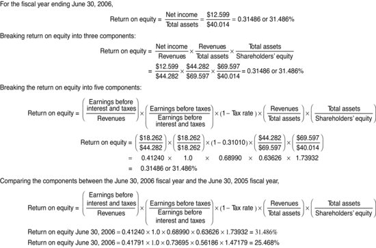
The analyst can decompose the return on equity further by breaking out the equity’s share of before-tax earnings (represented by the ratio of earnings before and after interest) and tax retention percentage. Consider the example in Figure 1, in which we provide a DuPont breakdown of the return on equity for Microsoft Corporation for the fiscal year ending June 30, 2006, in Panel A. The return on equity of 31.486% can be broken down into three and then five components, as shown in this figure. We can also use this breakdown to compare the return on equity for the 2005 and 2006 fiscal years, as shown in Panel B. As you can see, the return on equity improved from 2005 to 2006 and, using this breakdown, we can see that this was due primarily to the improvement in the asset turnover and the increased financial leverage.
Figure 1 The DuPont System Applied to Microsoft Corporation
This decomposition allows the analyst to take a closer look at the factors that are controllable by a company’s management (e.g., asset turnover) and those that are not controllable (e.g., tax retention). The breakdowns lead the analyst to information on both the balance sheet and the income statement. And this is not the only breakdown of the return ratios—further decomposition is possible.
LIQUIDITY
Liquidity reflects the ability of a firm to meet its short-term obligations using those assets that are most readily converted into cash. Assets that may be converted into cash in a short period of time are referred to as liquid assets; they are listed in financial statements as current assets. Current assets are often referred to as working capital, since they represent the resources needed for the day-to-day operations of the firm’s long-term capital investments. Current assets are used to satisfy short-term obligations, or current liabilities. The amount by which current assets exceed current liabilities is referred to as the net working capital.
Operating Cycle
How much liquidity a firm needs depends on its operating cycle. The operating cycle is the duration from the time cash is invested in goods and services to the time that investment produces cash. For example, a firm that produces and sells goods has an operating cycle comprising four phases:
The four phases make up the cycle of cash use and generation. The operating cycle would be somewhat different for companies that produce services rather than goods, but the idea is the same—the operating cycle is the length of time it takes to generate cash through the investment of cash.
What does the operating cycle have to do with liquidity? The longer the operating cycle, the more current assets are needed (relative to current liabilities) since it takes longer to convert inventories and receivables into cash. In other words, the longer the operating cycle, the greater the amount of net working capital required.
To measure the length of an operating cycle we need to know:
- The time it takes to convert the investment in inventory into sales (that is, cash → inventory → sales → accounts receivable).
- The time it takes to collect sales on credit (that is, accounts receivable → cash).
We can estimate the operating cycle for Fictitious Corporation for the current year, using the balance sheet and income statement data. The number of days Fictitious ties up funds in inventory is determined by the total amount of money represented in inventory and the average day’s cost of goods sold. The current investment in inventory—that is, the money “tied up” in inventory—is the ending balance of inventory on the balance sheet. The average day’s cost of goods sold is the cost of goods sold on an average day in the year, which can be estimated by dividing the cost of goods sold (which is found on the income statement) by the number of days in the year. The average day’s cost of goods sold for the current year is:
In other words, Fictitious incurs, on average, a cost of producing goods sold of $17,808 per day.
Fictitious has $1.8 million of inventory on hand at the end of the year. How many days’ worth of goods sold is this? One way to look at this is to imagine that Fictitious stopped buying more raw materials and just finished producing whatever was on hand in inventory, using available raw materials and work-in-process. How long would it take Fictitious to run out of inventory?
We compute the days sales in inventory (DSI), also known as the number of days of inventory, by calculating the ratio of the amount of inventory on hand (in dollars) to the average day’s cost of goods sold (in dollars per day):
In other words, Fictitious has approximately 101 days of goods on hand at the end of the current year. If sales continued at the same price, it would take Fictitious 101 days to run out of inventory.
If the ending inventory is representative of the inventory throughout the year, then it takes about 101 days to convert the investment in inventory into sold goods. Why worry about whether the year-end inventory is representative of inventory at any day throughout the year? Well, if inventory at the end of the fiscal year-end is lower than on any other day of the year, we have understated the DSI. Indeed, in practice most companies try to choose fiscal year-ends that coincide with the slow period of their business. That means the ending balance of inventory would be lower than the typical daily inventory of the year. To get a better picture of the firm, we could, for example, look at quarterly financial statements and take averages of quarterly inventory balances. However, here for simplicity we make a note of the problem of representatives and deal with it later in the discussion of financial ratios.
It should be noted that as an attempt to make the inventory figure more representative, some suggest taking the average of the beginning and ending inventory amounts. This does nothing to remedy the representativeness problem because the beginning inventory is simply the ending inventory from the previous year and, like the ending value from the current year, is measured at the low point of the operating cycle. A preferred method, if data are available, is to calculate the average inventory for the four quarters of the fiscal year.
We can extend the same logic for calculating the number of days between a sale—when an account receivable is created—and the time it is collected in cash. If we assume that Fictitious sells all goods on credit, we can first calculate the average credit sales per day and then figure out how many days’ worth of credit sales are represented by the ending balance of receivables.
The average credit sales per day are:
Therefore, Fictitious generates $27,397 of credit sales per day. With an ending balance of accounts receivable of $600,000, the days sales outstanding (DSO), also known as the number of days of credit, in this ending balance is calculated by taking the ratio of the balance in the accounts receivable account to the credit sales per day:
If the ending balance of receivables at the end of the year is representative of the receivables on any day throughout the year, then it takes, on average, approximately 22 days to collect the accounts receivable. In other words, it takes 22 days for a sale to become cash.
Using what we have determined for the inventory cycle and cash cycle, we see that for Fictitious:
We also need to look at the liabilities on the balance sheet to see how long it takes a firm to pay its short-term obligations. We can apply the same logic to accounts payable as we did to accounts receivable and inventories. How long does it take a firm, on average, to go from creating a payable (buying on credit) to paying for it in cash?
First, we need to determine the amount of an average day’s purchases on credit. If we assume all the Fictitious purchases are made on credit, then the total purchases for the year would be the cost of goods sold less any amounts included in cost of goods sold that are not purchases. For example, depreciation is included in the cost of goods sold yet is not a purchase. Since we do not have a breakdown on the company’s cost of goods sold showing how much was paid for in cash and how much was on credit, let us assume for simplicity that purchases are equal to cost of goods sold less depreciation. The average day’s purchases then become:
The days payables outstanding (DPO), also known as the number of days of purchases, represented in the ending balance in accounts payable, is calculated as the ratio of the balance in the accounts payable account to the average day’s purchases:
For Fictitious in the current year:
This means that on average Fictitious takes 33 days to pay out cash for a purchase.
The operating cycle tells us how long it takes to convert an investment in cash back into cash (by way of inventory and accounts receivable). The number of days of payables tells us how long it takes to pay on purchases made to create the inventory. If we put these two pieces of information together, we can see how long, on net, we tie up cash. The difference between the operating cycle and the number of days of purchases is the cash conversion cycle (CCC), also known as the net operating cycle:
![]()
Or, substituting for the operating cycle,
![]()
The cash conversion cycle for Fictitious in the current year is:
![]()
The CCC is how long it takes for the firm to get cash back from its investments in inventory and accounts receivable, considering that purchases may be made on credit. By not paying for purchases immediately (that is, using trade credit), the firm reduces its liquidity needs. Therefore, the longer the net operating cycle, the greater the required liquidity.
Measures of Liquidity
The analyst can describe a firm’s ability to meet its current obligations in several ways. The current ratio indicates the firm’s ability to meet or cover its current liabilities using its current assets:
![]()
For the Fictitious Corporation, the current ratio for the current year is the ratio of current assets, $3 million, to current liabilities, the sum of accounts payable and other current liabilities, or $1 million.
![]()
The current ratio of 3.0 indicates that Fictitious has three times as much as it needs to cover its current obligations during the year. However, the current ratio groups all current asset accounts together, assuming they are all as easily converted to cash. Even though, by definition, current assets can be transformed into cash within a year, not all current assets can be transformed into cash in a short period of time.
An alternative to the current ratio is the quick ratio, also called the acid-test ratio, which uses a slightly different set of current accounts to cover the same current liabilities as in the current ratio. In the quick ratio, the least liquid of the current asset accounts, inventory, is excluded. Hence:
![]()
We typically leave out inventories in the quick ratio because inventories are generally perceived as the least liquid of the current assets. By leaving out the least liquid asset, the quick ratio provides a more conservative view of liquidity.
For Fictitious in the current year:
Still another way to measure the firm’s ability to satisfy short-term obligations is the net working capital–to-sales ratio, which compares net working capital (current assets less current liabilities) with sales:
This ratio tells us the “cushion” available to meet short-term obligations relative to sales. Consider two firms with identical working capital of $100,000, but one has sales of $500,000 and the other sales of $1 million. If they have identical operating cycles, this means that the firm with the greater sales has more funds flowing in and out of its current asset investments (inventories and receivables). The company with more funds flowing in and out needs a larger cushion to protect itself in case of a disruption in the cycle, such as a labor strike or unexpected delays in customer payments. The longer the operating cycle, the more of a cushion (net working capital) a firm needs for a given level of sales.
For Fictitious Corporation:
The ratio of 0.20 tells us that for every dollar of sales, Fictitious has 20 cents of net working capital to support it.
Recap: Liquidity Ratios
Operating cycle and liquidity ratio information for Fictitious using data for the current year, in summary, is:
Days sales in inventory = 101 days
Days sales outstanding = 22 days
Operating cycle = 123 days
Days payables outstanding = 33 days
Cash conversion cycle = 90 days
Current ratio = 3.0
Quick ratio = 1.2
Net working capital–to-sales ratio = 20%
Given the measures of time related to the current accounts—the operating cycle and the cash conversion cycle—and the three measures of liquidity—current ratio, quick ratio, and net working capital–to-sales ratio—we know the following about Fictitious Corporation’s ability to meet its short-term obligations:
- Inventory is less liquid than accounts receivable (comparing days of inventory with days of credit).
- Current assets are greater than needed to satisfy current liabilities in a year (from the current ratio).
- The quick ratio tells us that Fictitious can meet its short-term obligations even without resorting to selling inventory.
- The net working capital “cushion” is 20 cents for every dollar of sales (from the net working capital–to-sales ratio.)
What don’t ratios tells us about liquidity? They don’t provide us with answers to the following questions:
- How liquid are the accounts receivable? How much of the accounts receivable will be collectible? Whereas we know it takes, on average, 22 days to collect, we do not know how much will never be collected.
- What is the nature of the current liabilities? How much of current liabilities consists of items that recur (such as accounts payable and wages payable) each period and how much consists of occasional items (such as income taxes payable)?
- Are there any unrecorded liabilities (such as operating leases) that are not included in current liabilities?
PROFITABILITY RATIOS
Liquidity ratios indicate a firm’s ability to meet its immediate obligations. Now we extend the analysis by adding profitability ratios, which help the analyst gauge how well a firm is managing its expenses. Profit margin ratios compare components of income with sales. They give the analyst an idea of which factors make up a firm’s income and are usually expressed as a portion of each dollar of sales. For example, the profit margin ratios we discuss here differ only in the numerator. It is in the numerator that we can evaluate performance for different aspects of the business.
For example, suppose the analyst wants to evaluate how well production facilities are managed. The analyst would focus on gross profit (sales less cost of goods sold), a measure of income that is the direct result of production management. Comparing gross profit with sales produces the gross profit margin:
This ratio tells us the portion of each dollar of sales that remains after deducting production expenses. For Fictitious Corporation for the current year:
For each dollar of revenues, the firm’s gross profit is 35 cents. Looking at sales and cost of goods sold, we can see that the gross profit margin is affected by:
- Changes in sales volume, which affect cost of goods sold and sales.
- Changes in sales price, which affect revenues.
- Changes in the cost of production, which affect cost of goods sold.
Any change in gross profit margin from one period to the next is caused by one or more of those three factors. Similarly, differences in gross margin ratios among firms are the result of differences in those factors.
To evaluate operating performance, we need to consider operating expenses in addition to the cost of goods sold. To do this, remove operating expenses (e.g., selling and general administrative expenses) from gross profit, leaving operating profit, also referred to as earnings before interest and taxes (EBIT). The operating profit margin is therefore:
For Fictitious in the current year:
Therefore, for each dollar of revenues, Fictitious has 20 cents of operating income. The operating profit margin is affected by the same factors as gross profit margin, plus operating expenses such as:
- Office rent and lease expenses
- Miscellaneous income (e.g., income from investments)
- Advertising expenditures
- Bad debt expense
Most of these expenses are related in some way to revenues, though they are not included directly in the cost of goods sold. Therefore, the difference between the gross profit margin and the operating profit margin is due to these indirect items that are included in computing the operating profit margin.
Both the gross profit margin and the operating profit margin reflect a company’s operating performance. But they do not consider how these operations have been financed. To evaluate both operating and financing decisions, the analyst must compare net income (that is, earnings after deducting interest and taxes) with revenues. The result is the net profit margin:
![]()
The net profit margin tells the analyst the net income generated from each dollar of revenues; it considers financing costs that the operating profit margin does not consider. For Fictitious for the current year:
![]()
For every dollar of revenues, Fictitious generates 12 cents in profits.
Recap: Profitability Ratios
The profitability ratios for Fictitious in the current year are:
Gross profit margin = 35%
Operating profit margin = 20%
Net profit margin = 12%
They indicate the following about the operating performance of Fictitious:
- Each dollar of revenues contributes 35 cents to gross profit and 20 cents to operating profit.
- Every dollar of revenues contributes 12 cents to owners’ earnings.
- By comparing the 20-cent operating profit margin with the 12-cent net profit margin, we see that Fictitious has 8 cents of financing costs for every dollar of revenues.
What these ratios do not indicate about profitability is the sensitivity of gross, operating, and net profit margins to:
- Changes in the sales price
- Changes in the volume of sales
Looking at the profitability ratios for one firm for one period gives the analyst very little information that can be used to make judgments regarding future profitability. Nor do these ratios provide the analyst any information about why current profitability is what it is. We need more information to make these kinds of judgments, particularly regarding the future profitability of the firm. For that, turn to activity ratios, which are measures of how well assets are being used.
ACTIVITY RATIOS
Activity ratios—for the most part, turnover ratios—can be used to evaluate the benefits produced by specific assets, such as inventory or accounts receivable, or to evaluate the benefits produced by the totality of the firm’s assets.
Inventory Management
The inventory turnover ratio indicates how quickly a firm has used inventory to generate the goods and services that are sold. The inventory turnover is the ratio of the cost of goods sold to inventory:
![]()
For Fictitious for the current year:
This ratio indicates that Fictitious turns over its inventory 3.61 times per year. On average, cash is invested in inventory, goods and services are produced, and these goods and services are sold 3.6 times a year. Looking back to the number of days of inventory, we see that this turnover measure is consistent with the results of that calculation: There are 101 calendar days of inventory on hand at the end of the year; dividing 365 days by 101 days, or 365/101 days, we find that inventory cycles through (from cash to sales) 3.61 times a year.
Accounts Receivable Management
In much the same way inventory turnover can be evaluated, an analyst can evaluate a firm’s management of its accounts receivable and its credit policy. The accounts receivable turnover ratio is a measure of how effectively a firm is using credit extended to customers. The reason for extending credit is to increase sales. The downside to extending credit is the possibility of default—customers not paying when promised. The benefit obtained from extending credit is referred to as net credit sales—sales on credit less returns and refunds.
![]()
Looking at the Fictitious Corporation income statement, we see an entry for sales, but we do not know how much of the amount stated is on credit. In the case of evaluating a firm, an analyst would have an estimate of the amount of credit sales. Let us assume that the entire sales amount represents net credit sales. For Fictitious for the current year:
Therefore, almost 17 times in the year there is, on average, a cycle that begins with a sale on credit and finishes with the receipt of cash for that sale. In other words, there are 17 cycles of sales to credit to cash during the year.
The number of times accounts receivable cycle through the year is consistent with the days sales outstanding (22) that we calculated earlier—accounts receivable turn over 17 times during the year, and the average number of days of sales in the accounts receivable balance is 365 days/16.67 times = 22 days.
Overall Asset Management
The inventory and accounts receivable turnover ratios reflect the benefits obtained from the use of specific assets (inventory and accounts receivable). For a more general picture of the productivity of the firm, an analyst can compare the sales during a period with the total assets that generated these revenues.
One way is with the total asset turnover ratio, which indicates how many times during the year the value of a firm’s total assets is generated in revenues:
![]()
For Fictitious in the current year:
The turnover ratio of 0.91 indicated that in the current year, every dollar invested in total assets generates 91 cents of sales. Or, stated differently, the total assets of Fictitious turn over almost once during the year. Because total assets include both tangible and intangible assets, this turnover indicates how efficiently all assets were used.
An alternative is to focus only on fixed assets, the long-term, tangible assets of the firm. The fixed-asset turnover is the ratio of revenues to fixed assets:
![]()
For Fictitious in the current year:
Therefore, for every dollar of fixed assets, Fictitious is able to generate $1.43 of revenues.
Recap: Activity Ratios
The activity ratios for Fictitious Corporation are:
From these ratios the analyst can determine that:
- Inventory flows in and out almost four times a year (from the inventory turnover ratio).
- Accounts receivable are collected in cash, on average, 22 days after a sale (from the number of days of credit). In other words, accounts receivable flow in and out almost 17 times during the year (from the accounts receivable turnover ratio).
Here is what these ratios do not indicate about the firm’s use of its assets:
- The sales not made because credit policies are too stringent.
- How much of credit sales is not collectible.
- Which assets contribute most to the turnover.
FINANCIAL LEVERAGE RATIOS
A firm can finance its assets with equity or with debt. Financing with debt legally obligates the firm to pay interest and to repay the principal as promised. Equity financing does not obligate the firm to pay anything because dividends are paid at the discretion of the board of directors. There is always some risk, which we refer to as business risk, inherent in any business enterprise. But how a firm chooses to finance its operations—the particular mix of debt and equity—may add financial risk on top of business risk. Financial risk is risk associated with a firm’s ability to satisfy its debt obligations, and is often measured using the extent to which debt financing is used relative to equity.
Financial leverage ratios are used to assess how much financial risk the firm has taken on. There are two types of financial leverage ratios: component percentages and coverage ratios. Component percentages compare a firm’s debt with either its total capital (debt plus equity) or its equity capital. Coverage ratios reflect a firm’s ability to satisfy fixed financing obligations, such as interest, principal repayment, or lease payments.
Component Percentage Ratios
A ratio that indicates the proportion of assets financed with debt is the debt-to-assets ratio, which compares total liabilities (short-term + long-term debt) with total assets:
![]()
For Fictitious in the current year:
This ratio indicates that 45% of the firm’s assets are financed with debt (both short term and long term).
Another way to look at the financial risk is in terms of the use of debt relative to the use of equity. The debt-to-equity ratio indicates how the firm finances its operations with debt relative to the book value of its shareholders’ equity:
For Fictitious for the current year, using the book-value definition:
For every $1 of book value of shareholders’ equity, Fictitious uses 83 cents of debt.
Both of these ratios can be stated in terms of total debt, as above, or in terms of long-term debt or even simply interest-bearing debt. And it is not always clear in which form—total, long-term debt, or interest-bearing—the ratio is calculated. Additionally, it is often the case that the current portion of long-term debt is excluded in the calculation of the long-term versions of these debt ratios.
Book Value versus Market Value
One problem with using a financial ratio based on the book value of equity to analyze financial risk is that there is seldom a strong relationship between the book value and market value of a stock. The distortion in values on the balance sheet is obvious by looking at the book value of equity and comparing it with the market value of equity. The book value of equity consists of:
- The proceeds to the firm of all the stock issues since it was first incorporated, less any stock repurchased by the firm.
- The accumulative earnings of the firm, less any dividends, since it was first incorporated.
Let’s look at an example of the book value versus the market value of equity. IBM was incorporated in 1911, so the book value of its equity represents the sum of all its stock issued and all its earnings, less any dividends paid since 1911. As of the end of 2006, IBM’s book value of equity was approximately $28.5 billion, yet its market value was $142.8 billion.
Book value generally does not give a true picture of the investment of shareholders in the firm because:
- Earnings are recorded according to accounting principles, which may not reflect the true economics of transactions.
- Due to inflation, the earnings and proceeds from stock issued in the past do not reflect today’s values.
Market value, on the other hand, is the value of equity as perceived by investors. It is what investors are willing to pay. So why bother with book value? For two reasons: First, it is easier to obtain the book value than the market value of a firm’s securities, and second, many financial services report ratios using book value rather than market value.
However, any of the ratios presented in this entry that use the book value of equity can be restated using the market value of equity. For example, instead of using the book value of equity in the debt-to-equity ratio, the market value of equity to measure the firm’s financial leverage can be used.
Coverage Ratios
The ratios that compare debt to equity or debt to assets indicate the amount of financial leverage, which enables an analyst to assess the financial condition of a firm. Another way of looking at the financial condition and the amount of financial leverage used by the firm is to see how well it can handle the financial burdens associated with its debt or other fixed commitments.
One measure of a firm’s ability to handle financial burdens is the interest coverage ratio, also referred to as the times interest-covered ratio. This ratio tells us how well the firm can cover or meet the interest payments associated with debt. The ratio compares the funds available to pay interest (that is, earnings before interest and taxes) with the interest expense:
![]()
The greater the interest coverage ratio, the better able the firm is to pay its interest expense. For Fictitious for the current year:
![]()
An interest coverage ratio of 5 means that the firm’s earnings before interest and taxes are five times greater than its interest payments.
The interest coverage ratio provides information about a firm’s ability to cover the interest related to its debt financing. However, there are other costs that do not arise from debt but that nevertheless must be considered in the same way we consider the cost of debt in a firm’s financial obligations. For example, lease payments are fixed costs incurred in financing operations. Like interest payments, they represent legal obligations.
What funds are available to pay debt and debt-like expenses? Start with EBIT and add back expenses that were deducted to arrive at EBIT. The ability of a firm to satisfy its fixed financial costs—its fixed charges—is referred to as the fixed-charge coverage ratio. One definition of the fixed-charge coverage considers only the lease payments:
For Fictitious for the current year:
This ratio tells us that Fictitious’s earnings can cover its fixed charges (interest and lease payments) more than two times over.
What fixed charges to consider is not entirely clear-cut. For example, if the firm is required to set aside funds to eventually or periodically retire debt—referred to as sinking funds—is the amount set aside a fixed charge? As another example, since preferred dividends represent a fixed financing charge, should they be included as a fixed charge? From the perspective of the common shareholder, the preferred dividends must be covered either to enable the payment of common dividends or to retain earnings for future growth. Because debt principal repayment and preferred stock dividends are paid on an after-tax basis—paid out of dollars remaining after taxes are paid—this fixed charge must be converted to before-tax dollars. The fixed charge coverage ratio can be expanded to accommodate the sinking funds and preferred stock dividends as fixed charges.
Up to now we considered earnings before interest and taxes as funds available to meet fixed financial charges. EBIT includes noncash items such as depreciation and amortization. If an analyst is trying to compare funds available to meet obligations, a better measure of available funds is cash flow from operations, as reported in the statement of cash flows. A ratio that considers cash flows from operations as funds available to cover interest payments is referred to as the cash-flow interest coverage ratio.
The amount of cash flow from operations that is in the statement of cash flows is net of interest and taxes. So we have to add back interest and taxes to cash flow from operations to arrive at the cash flow amount before interest and taxes in order to determine the cash flow available to cover interest payments.
For Fictitious for the current year:
This coverage ratio indicates that, in terms of cash flows, Fictitious has 6.5 times more cash than is needed to pay its interest. This is a better picture of interest coverage than the five times reflected by EBIT. Why the difference? Because cash flow considers not just the accounting income, but noncash items as well. In the case of Fictitious, depreciation is a noncash charge that reduced EBIT but not cash flow from operations—it is added back to net income to arrive at cash flow from operations.
Recap: Financial Leverage Ratios
Summarizing, the financial leverage ratios for Fictitious Corporation for the current year are:
These ratios indicate that Fictitious uses its financial leverage as follows:
- Assets are 45% financed with debt, measured using book values.
- Long-term debt is approximately two-thirds of equity. When equity is measured in market value terms, long-term debt is approximately one-sixth of equity.
These ratios do not indicate:
- What other fixed, legal commitments the firm has that are not included on the balance sheet (for example, operating leases).
- What the intentions of management are regarding taking on more debt as the existing debt matures.
COMMON-SIZE ANALYSIS
An analyst can evaluate a company’s operating performance and financial condition through ratios that relate various items of information contained in the financial statements. Another way to analyze a firm is to look at its financial data more comprehensively.
Table 4 Fictitious Corporation Common-Size Balance Sheets for Years Ending December 31
Common-size analysis is a method of analysis in which the components of a financial statement are compared with each other. The first step in common-size analysis is to break down a financial statement—either the balance sheet or the income statement—into its parts. The next step is to calculate the proportion that each item represents relative to some benchmark. This form of common-size analysis is sometimes referred to as vertical common-size analysis. Another form of common-size analysis is horizontal common-size analysis, which uses either an income statement or a balance sheet in a fiscal year and compares accounts to the corresponding items in another year. In common-size analysis of the balance sheet, the benchmark is total assets. For the income statement, the benchmark is sales.
Let us see how it works by doing some common-size financial analysis for the Fictitious Corporation. The company’s balance sheet is restated in Table 4. This statement does not look precisely like the balance sheet we have seen before. Nevertheless, the data are the same but reorganized. Each item in the original balance sheet has been restated as a proportion of total assets for the purpose of common size analysis. Hence, we refer to this as the common-size balance sheet.
Table 5 Fictitious Corporation Common-Size Income Statement for Years Ending December 31
| Current | Prior | |
| Year | Year | |
| Sales | 100.0% | 100.0% |
| Cost of goods sold | 65.0% | 66.7% |
| Gross profit | 35.0% | 33.3% |
| Lease and administrative expenses | 15.0% | 11.1% |
| Earnings before interest and taxes | 20.0% | 22.2% |
| Interest expense | 4.0% | 5.6% |
| Earnings before taxes | 16.0% | 16.6% |
| Taxes | 4.0% | 5.5% |
| Net income | 12.0% | 11.1% |
| Common dividends | 6.0% | 5.6% |
| Retained earnings | 6.0% | 5.5% |
In this balance sheet, we see, for example, that in the current year cash is 3.6% of total assets, or $400,000/$11,000,000 = 0.036. The largest investment is in plant and equipment, which comprises 63.6% of total assets. On the liabilities side, that current liabilities are a small portion (9.1%) of liabilities and equity.
The common-size balance sheet indicates in very general terms how Fictitious has raised capital and where this capital has been invested. As with financial ratios, however, the picture is not complete until trends are examined and compared with those of other firms in the same industry.
In the income statement, as with the balance sheet, the items may be restated as a proportion of sales; this statement is referred to as the common-size income statement. The common-size income statements for Fictitious for the two years are shown in Table 5. For the current year, the major costs are associated with goods sold (65%); lease expense, other expenses, interest, taxes, and dividends make up smaller portions of sales. Looking at gross profit, EBIT, and net income, these proportions are the profit margins we calculated earlier. The common-size income statement provides information on the profitability of different aspects of the firm’s business. Again, the picture is not yet complete. For a more complete picture, the analyst must look at trends over time and make comparisons with other companies in the same industry.
USING FINANCIAL RATIO ANALYSIS
Financial analysis provides information concerning a firm’s operating performance and financial condition. This information is useful for an analyst in evaluating the performance of the company as a whole, as well as of divisions, products, and subsidiaries. An analyst must also be aware that financial analysis is also used by analysts and investors to gauge the financial performance of the company.
But financial ratio analysis cannot tell the whole story and must be interpreted and used with care. Financial ratios are useful but, as noted in the discussion of each ratio, there is information that the ratios do not reveal. For example, in calculating inventory turnover, we need to assume that the inventory shown on the balance sheet is representative of inventory throughout the year. Another example is in the calculation of accounts receivable turnover. We assumed that all sales were on credit. If we are on the outside looking in—that is, evaluating a firm based on its financial statements only, such as the case of a financial analyst or investor—and therefore do not have data on credit sales, assumptions must be made that may or may not be correct.
In addition, there are other areas of concern that an analyst should be aware of in using financial ratios:
- Limitations in the accounting data used to construct the ratios.
- Selection of an appropriate benchmark firm or firms for comparison purposes.
- Interpretation of the ratios.
- Pitfalls in forecasting future operating performance and financial condition based on past trends.
KEY POINTS
- The basic data for financial analysis are the financial statement data. These data are used to analyze relationships between different elements of a firm’s financial statements. Through this analysis, a picture of the operating performance and financial condition of a firm can be developed.
- Looking at the calculated financial ratios, in conjunction with industry and economic data, judgments about past and future financial performance and condition can be made.
- Financial ratios can be classified by type—coverage, return, turnover, or component percentage—or by the financial characteristic that we wish to measure—liquidity, profitability activity, financial leverage, or return.
- Liquidity ratios indicate firm’s ability to satisfy short-term obligations. These ratios are closely related to a firm’s operating cycle, which tells us how long it takes a firm to turn its investment in current assets back into cash.
- Profitability ratios indicate how well a firm manages its assets, typically in terms of the proportion of revenues that are left over after expenses.
- Activity ratios measure how efficiently a firm manages its assets, that is, how effectively a firm uses its assets to generate sales.
- Financial leverage ratios indicate (1) to what extent a firm uses debt to finance its operations and (2) its ability to satisfy debt and debt-like obligations.
- Return-on-investment ratios provide a gauge for how much of each dollar of an investment is generated in a period.
- The DuPont system breaks down return ratios into their profit margin and activity ratios, allowing us to analyze changes in return on investments.
- Common-size analysis expresses financial statement data relative to some benchmark item—usually total assets for the balance sheet and sales for the income statement. Representing financial data in this way allows an analyst to spot trends in investments and profitability.
- Interpretation of financial ratios requires an analyst to put the trends and comparisons in perspective with the company’s significant events. In addition to company-specific events, issues that can cause the analysis of financial ratios to become more challenging include the use of historical accounting values, changes in accounting principles, and accounts that are difficult to classify.
- Comparison of financial ratios across time and with competitors is useful in gauging performance. In comparing ratios over time, an analyst should consider changes in accounting and significant company events. In comparing ratios with a benchmark, an analyst must take care in the selection of the companies that constitute the benchmark and the method of calculation.
REFERENCES
Bernstein, L. A. (1999). Analysis of Financial Statements, 5th edition. New York: McGraw-Hill.
Fabozzi, F. J., Drake, P. P., and Polimeni, R. S. (2007). The Complete CFO Handbook: From Accounting to Accountability. Hoboken, NJ: John Wiley & Sons.
Fridson, M., and Alvarez, F. (2011). Financial Statement Analysis: A Practitioner’s Guide, 4th edition. Hoboken, NJ: John Wiley & Sons.
Peterson, P. P., and Fabozzi, F. J. (2012). Analysis of Financial Statements, 3rd edition. Hoboken, NJ: John Wiley & Sons.