Equity Portfolio Selection Models in Practice

DESSISLAVA A. PACHAMANOVA, PhD

Associate Professor of Operations Research, Babson College

FRANK J. FABOZZI, PhD, CFA, CPA

Professor of Finance, EDHEC Business School

An integrated investment process generally involves the following activities:1

In this entry we focus on the second activity of the investment process, developing and implementing a portfolio strategy. The development of the portfolio strategy itself is typically done in two stages: First, funds are allocated among asset classes. Then, they are managed within the asset classes. The mean-variance framework is used at both stages, but in this entry, we discuss the second stage. Specifically, we introduce quantitative formulations of portfolio allocation problems used in equity portfolio management. Quantitative equity portfolio selection often involves extending the classical mean-variance framework or more advanced tail-risk portfolio allocation frameworks to include different constraints that take specific investment guidelines and institutional features into account.

We begin by providing a classification of the most common portfolio constraints used in practice. We then discuss extensions such as index tracking formulations, the inclusion of transaction costs, optimization of trades across multiple client accounts, and tax-aware strategies. We conclude with a review of methods for incorporating robustness in quantitative portfolio allocation procedures by using robust statistics, simulation, and robust optimization techniques.

PORTFOLIO CONSTRAINTS COMMONLY USED IN PRACTICE

Institutional features and investment policy specifications often lead to more complicated requirements than simple minimization of risk (whatever the definition of risk may be) or maximization of expected portfolio return. For instance, there can be constraints that limit the number of trades, the exposure to a specific industry, or the number of stocks to be kept in the portfolio. Some of these constraints are imposed by the clients, while others are imposed by regulators. For example, in the case of regulated investment companies, restrictions on asset allocation are set forth in the prospectus and may be changed only with the approval of the fund’s board of directors. Pension funds must comply with Employee Retirement Income Security Act (ERISA) requirements. The objective of the portfolio optimization problem can also be modified to consider specifically the trade-off between risk and return, transactions costs, or taxes.

In this section, we will take a single-period view of investing, in the sense that the goal of the portfolio allocation procedure will be to invest optimally over a single predetermined period of interest, such as one month.2 We will use w0 to denote the vector array of stock weights in the portfolio at the beginning of the period, and w to denote the weights at the end of the period (to be determined).

Many investment companies, especially institutional investors, have a long investment horizon. However, in reality, they treat that horizon as a sequence of shorter period horizons. Risk budgets are often stated over a time period of a year, and return performance is monitored quarterly or monthly.

Long-Only (No-Short-Selling) Constraints

Many funds and institutional investors face restrictions or outright prohibitions on the amount of short selling they can do. When short selling is not allowed, the portfolio allocation optimization model contains the constraints w ≥ 0.

Holding Constraints

Diversification principles argue against investing a large proportion of the portfolio in a single asset, or having a large concentration of assets in a specific industry, sector, or country. Limits on the holdings of a specific stock can be imposed with the constraints

where l and u are vectors of lower and upper bounds of the holdings of each stock in the portfolio.

Consider now a portfolio of 10 stocks. Suppose that the issuers of assets 1, 3, and 5 are in the same industry, and that we would like to limit the portfolio exposure to that industry to be at least 20% but at most 40%. To limit exposure to that industry, we add the constraint

to the portfolio allocation optimization problem.

More generally, if we have a specific set of stocks Ij out of the investment universe I consisting of stocks in the same category (such as industry or country), we can write the constraint

In words, this constraint requires that the sum of all stock weights in the particular category of investments with indexes Ij is greater than or equal to a lower bound Lj and less than or equal to a maximum exposure of Uj.

Turnover Constraints

High portfolio turnover can result in large transaction costs that make portfolio rebalancing inefficient and costly. Thus, some portfolio managers limit the amount of turnover allowed when trading their portfolio. (Another way to control for transaction costs is to minimize them explicitly; we will discuss the appropriate formulations later in this entry.)

Most commonly, turnover constraints are imposed for each stock:

that is, the absolute magnitude of the difference between the final and the initial weight of stock i in the portfolio is restricted to be less than some upper bound ui. Sometimes, a constraint is imposed to minimize the portfolio turnover as a whole:

that is, the total absolute difference between the initial and the final weights of the stocks in the portfolio is restricted to be less than or equal to an upper bound Ui. Under this constraint, some stock weights may deviate a lot more than others from their initial weights, but the total deviation is limited.

Turnover constraints are often imposed relative to the average daily volume (ADV) of a stock.3 For example, we may want to restrict turnover to be no more than 5% of the ADV. (In the latter case, the upper bound ui is set to a value equal to 5% of the ADV.) Modifications of these constraints, such as limiting turnover in a specific industry or sector, are also frequently applied.

Risk Factor Constraints

In practice, it is very common for quantitatively oriented portfolio managers to use factor models to control for risk exposures to different risk factors. Such risk factors could include the market return, size, and style. Let us assume that the return on stock i has a factor structure with K risk factors, that is, it can be expressed through the equality

The factors fk are common to all securities. The coefficient βik in front of each factor fk shows the sensitivity of the return on stock i to factor k. The value of αi shows the expected excess return of the return on stock i, and εi is the idiosyncratic (called “nonsystematic”) part of the return of stock i. The coefficients αi and βik are typically estimated by multiple regression analysis.

To limit the exposure of a portfolio of N stocks to the kth risk factor, we impose the constraint

To understand this constraint, note that the total return on the portfolio can be written as

The sensitivity of the portfolio to the different factors is represented by the second term, which can be also written as

Therefore, the exposure to a particular factor k is the coefficient in front of fk, that is,

On an intuitive level, the sensitivity of the portfolio to a factor k will be larger the larger the presence of factor k in the portfolio through the exposure of the individual stocks. Thus, when we compute the total exposure of the portfolio to factor k, we need to take into consideration both how important this factor is for determining the return on each of the securities in the portfolio, and how much of each security we have in the portfolio.

A commonly used version of the maximum factor exposure constraint is

This constraint forces the portfolio optimization algorithm to find portfolio weights so that the overall risk exposure to factor k is 0, that is, so that the portfolio is neutral with respect to changes in factor k. Portfolio allocation strategies that claim to be “market-neutral” typically employ this constraint, and the factor is in fact the return on the market.

Cardinality Constraints

Depending on the portfolio allocation model used, sometimes the optimization subroutine recommends holding small amounts of a large number of stocks, which can be costly when one takes into consideration the transaction costs incurred when acquiring these positions. Alternatively, a portfolio manager may be interested in limiting the number of stocks used to track a particular index. (We will discuss index tracking later in this entry.) To formulate the constraint on the number of stocks to be held in the portfolio (called the cardinality constraint), we introduce binary variables, one for each of the N stocks in the portfolio. Let us call these binary variables δ1, … , δN. Variable δi will take value 1 if stock i is included in the portfolio, and 0 otherwise.

Suppose that out of the N stocks in the investment universe, we would like to include a maximum of K stocks in the final portfolio. K here is a positive integer and is less than N. This constraint can be formulated as

We need to make sure, however, that if a stock is not selected in the portfolio, then the binary variable that corresponds to that stock is set to 0, so that the stock is not counted as one of the K stocks left in the portfolio. When the portfolio weights are restricted to be nonnegative, this can be achieved by imposing the additional constraints

If the optimal weight for stock i turns out to be different from 0, then the binary variable δi associated with stock i is forced to take value 1, and stock i will be counted as one of the K stocks to be kept in the portfolio. If the optimal weight for stock i is 0, then the binary variable δi associated with stock i can be either 0 or 1, but that will not matter for all practical purposes, because the solver will set it to 0 if there are too many other attractive stocks that will be counted as the K stocks to be kept in the portfolio. At the same time, since the portfolio weights wi are between 0 and 1, and δi is 0 or 1, the constraint wi ≤ δi does not restrict the values that the stock weight wi can take.

The constraints are a little different if short sales are allowed, in which case the weights may be negative. We have

where M is a “large” constant (large relative to the size of the inputs in the problem; so in this portfolio optimization application M = 10 can be considered “large”). You can observe that if the weight wi is anything but 0, the value of the binary variable δi will be forced to be different from 0, that is, δi will need to be 1, since it can only take values 0 or 1.

Minimum Holding and Transaction Size Constraints

Cardinality constraints are often used in conjunction with minimum holding/trading constraints. The latter set a minimum limit on the amount of a stock that can be held in the portfolio, or the amount of a stock that can be traded, effectively eliminating small trades. Both cardinality and minimum holding/trading constraints aim to reduce the amount of transaction costs.

Threshold constraints on the amount of stock i to be held in the portfolio can be imposed with the constraint

where Li is the smallest holding size allowed for stock i, and δi is a binary variable, analogous to the binary variables δi defined in the previous section—it equals 1 if stock i is included in the portfolio, and 0 otherwise. (All additional constraints relating δi and wi described in the previous section still apply.)

Similarly, constraints can be imposed on the minimum trading amount for stock i. As we explained earlier in this section, the size of the trade for stock i is determined by the absolute value of the difference between the current weight of the stock, w0,i, and the new weight wi that will be found by the solver: | wi – w0,i |. The minimum trading size constraint formulation is

where Ltradei is the smallest trading size allowed for stock i.

Adding binary variables to an optimization problem makes the problem more difficult for the solver and can increase the computation time substantially. That is why in practice, portfolio managers often omit minimum holding and transaction size constraints from the optimization problem formulation, selecting instead to eliminate weights and/or trades that appear too small manually, after the optimal portfolio is determined by the optimization solver. It is important to realize, however, that modifying the optimal solution for the simpler portfolio allocation problem (the optimal solution in this case is the weights/trades for the different stocks) by eliminating small positions manually does not necessarily produce the optimal solution to an optimization problem that contained the minimum holding and transaction size constraints from the beginning. In fact, there can be pathological cases in which the solution is very different from the true optimal solution. However, for most cases in practice, the small manual adjustments to the optimal portfolio allocation do not cause tremendous discrepancies or inconsistencies.

Round Lot Constraints

So far, we have assumed that stocks are infinitely divisible, that is, that we can trade and invest in fractions of stocks, bonds, and so on. This is, of course, not true—in reality, securities are traded in multiples of minimum transaction lots, or rounds (e.g., 100 or 500 shares).

In order to represent the condition that securities should be traded in rounds, we need to introduce additional decision variables (let us call them zi, i = 1, … , N) that are integers and will correspond to the number of lots of a particular security that will be purchased. Each zi will then be linked to the corresponding portfolio weight wi through the equality

where fi is measured in dollars, and is a fraction of the total amount to be invested. For example, suppose there is a total of $100 million to be invested, and stock i trades at $50 in round lots of 100. Then

All remaining constraints in the portfolio allocation can be expressed through the weights wi, as usual. However, we also need to specify for the solver that the decision variables zi are integers.

An issue with imposing round lot constraints is that the budget constraint

which is in fact

may not be satisfied exactly. One possibility to handle this problem is to relax the budget constraint. For example, we can state the constraint as

or, equivalently,

This will ensure that we do not go over budget.

If our objective is stated as expected return maximization, the optimization solver will attempt to make this constraint as tight as possible, that is, we will end up using up as much of the budget as we can. Depending on the objective function and the other constraints in the formulation, however, this may not always happen. We can try to force the solver to minimize the slack in the budget constraint by introducing a pair of nonnegative decision variables (let us call them ε+ and ε−) that account for the amount that is “overinvested” or “underinvested.” These variables will pick up the slack left over because of the inability to round the amounts for the different investments. Namely, we impose the constraints

and subtract the following term from the objective function:

where λrl is a penalty term associated with the amount of over- or underinvestment the portfolio manager is willing to tolerate (selected by the portfolio manager). In the final solution, the violation of the budget constraint will be minimized. Note, however, that this formulation technically allows for the budget to be overinvested.

The optimal portfolio allocation we obtain after solving this optimization problem will not be the same as the allocation we would obtain if we solve an optimization problem without round lot constraints, and then round the amounts to fit the lots that can be traded in the market.

Cardinality constraints, minimum holding/trading constraints, and especially round lot constraints require more sophisticated binary and integer programming solvers, and are difficult problems to solve in the case of large portfolios.

BENCHMARK EXPOSURE AND TRACKING ERROR MINIMIZATION

Expected portfolio return maximization under the mean-variance framework or other risk measure minimization are examples of active investment strategies, that is, strategies that identify a universe of attractive investments and ignore inferior investments opportunities. A different approach, referred to as a passive investment strategy, argues that in the absence of any superior forecasting ability, investors might as well resign themselves to the fact that they cannot beat the market. From a theoretical perspective, the analytics of portfolio theory tell them to hold a broadly diversified portfolio anyway. Many mutual funds are managed relative to a particular benchmark or stock universe, such as the S&P 500 or the Russell 1000. The portfolio allocation models are then formulated in such a way that the tracking error relative to the benchmark is kept small.

Standard Definition of Tracking Error

To incorporate a passive investment strategy, we can change the objective function of the portfolio allocation problem so that instead of minimizing a portfolio risk measure, we minimize the tracking error with respect to a benchmark that represents the market, such as the Russell 3000, or the S&P 500. Such strategies are often referred to as indexing. The tracking error can be defined in different ways. However, practitioners typically mean a specific definition: the variance (or standard deviation) of the difference between the portfolio return, , and the return on the benchmark . Mathematically, the tracking error (TE) can be expressed as

where is the covariance matrix of the stock returns. One can observe that the formula is very similar to the formula for the portfolio variance; however, the portfolio weights in the formula for the variance are replaced by differences between the weights of the stocks in the portfolio and the weights of the stocks in the index.

Why do we need to optimize portfolio weights in order to track a benchmark, when technically the most effective way to track a benchmark is by investing the portfolio in the stocks in the benchmark portfolio in the same proportions as the proportions of these securities in the benchmark? The problem with this approach is that, especially with large benchmarks like the Russell 3000, the transaction costs of a proportional investment and the subsequent rebalancing of the portfolio can be prohibitive (that is, dramatically adversely impact the performance of the portfolio relative to the benchmark). Furthermore, in practice securities are not infinitely divisible, so investing a portfolio of a limited size in the same proportions as the composition of the benchmark will still not achieve zero tracking error. Thus, the optimal formulation is to require that the portfolio follows the benchmark as closely as possible.

While indexing has become an essential part of many portfolio strategies, most portfolio managers cannot resist the temptation to identify at least some securities that will outperform others. Hence, restrictions on the tracking error are often imposed as a constraint, while the objective function is something different from minimizing the tracking error. The tracking error constraint takes the form

where is a limit (imposed by the investor) on the amount of tracking error the investor is willing to tolerate. This is a quadratic constraint, which is convex and computationally tractable, but requires specialized optimization software.

Alternative Ways of Defining Tracking Error

There are alternative ways in which tracking-error type constraints can be imposed.

For example, we may require that the absolute deviations of the portfolio weights (w) from the index weights (wb) are less than or equal to a given vector array of upper bounds u:

where the absolute values |.| for the vector differences are taken componentwise, that is, for pairs of corresponding elements from the two vector arrays. These constraints can be stated as linear constraints by rewriting them as

Similarly, we can require that for stocks within a specific industry (whose indexes in the portfolio belong to a subset Ij of the investment universe I), the total tracking error is less than a given upper bound Uj:

Finally, tracking error can be expressed through risk measures other than the absolute deviations or the variance of the deviations from the benchmark. Rockafellar and Uryasev (2000) suggest using conditional value-at-risk (CVaR) to manage the tracking error. Conditional value-at-risk measures the average loss that can happen with probability less than some small probability, that is, the average loss in the tail of the distribution of portfolio losses. (Using CVaR as a risk measure results in computationally tractable optimization formulations for portfolio allocation, as long as the data are presented in the form of scenarios.4) We provide below a formulation that is somewhat different from Rockafellar and Uryasev, but preserves the main idea.

Suppose that we are given S scenarios for the return of a benchmark portfolio (or an instrument we are trying to replicate), bs, s = 1, … , S. These scenarios can be generated by simulation or taken from historical data. We also have N stocks with returns r(s)i(i = 1, … , N, s = 1, … , S) in each scenario. The value of the portfolio in scenario s is

or, equivalently, (r(s))’w, where r(s) is the vector of returns for the N stocks in scenario s. Consider the differences between the return on the benchmark and the return on the portfolio,

If this difference is positive, we have a loss; if the difference is negative, we have a gain; both gains and losses are computed relative to the benchmark. Rationally, the portfolio manager should not worry about differences that are negative; the only cause for concern would be if the portfolio underperforms the benchmark, which would result in a positive difference. Thus, it is not necessary to limit the variance of the deviations of the portfolio returns from the benchmark, which penalizes for positive and negative deviations equally. Instead, we can impose a limit on the amount of loss we are willing to tolerate in terms of the CVaR of the distribution of losses relative to the benchmark.

The tracking error constraint in terms of the CVaR can be stated as the following set of constraints:5

where UTE is the upper bound on the negative deviations.

This formulation of tracking error is appealing in two ways. First, it treats positive and negative deviations relative to the benchmark differently, which agrees with the strategy of an investor seeking to maximize returns overall. Second, it results in a linear set of constraints, which are easy to handle computationally, in contrast to the first formulation of the tracking error constraint in this section, which results in a quadratic constraint.

Actual Versus Predicted Tracking Error

The tracking error calculation in practice is often backward-looking. For example, in computing the covariance matrix in the standard tracking error definition as the variance of the deviations of the portfolio returns from the index, or in selecting the scenarios used in the CVaR-type tracking error constraint in the previous section, we may use historical data. The tracking error calculated in this manner is called the ex post tracking error, backward-looking error, or actual tracking error.

The problem with using the actual tracking error for assessing future performance relative to a benchmark is that the actual tracking error does not reflect the effect of the portfolio manager’s current decisions on the future active returns and hence the tracking error that may be realized in the future. The actual tracking error has little predictive value and can be misleading regarding portfolio risk.

Portfolio managers need forward-looking estimates of tracking error to reflect future portfolio performance more accurately. In practice, this is accomplished by using the services of a commercial vendor that has a multifactor risk model that has identified and defined the risks associated with the benchmark, or by building such a model in-house. Statistical analysis of historical return data for the stocks in the benchmark is used to obtain the risk factors and to quantify the risks. Using the manager’s current portfolio holdings, the portfolio’s current exposure to the various risk factors can be calculated and compared to the benchmark’s exposures to the risk factors. From the differential factor exposures and the risks of the factors, a forward-looking tracking error for the portfolio can be computed. This tracking error is also referred to as an ex ante tracking error or predicted tracking error.

There is no guarantee that the predicted tracking error will match exactly the tracking error realized over the future time period of interest. However, this calculation of the tracking error has its use in risk control and portfolio construction. By performing a simulation analysis on the factors that enter the calculation, the manager can evaluate the potential performance of portfolio strategies relative to the benchmark, and eliminate those that result in tracking errors beyond the client-imposed tolerance for risk. The actual tracking error, on the other hand, is useful for assessing actual performance relative to a benchmark.

INCORPORATING TRANSACTION COSTS

Transaction costs can be generally divided into two categories: (1) explicit such as bid-ask spreads, commissions, and fees, and (2) implicit such as price movement risk costs and market impact costs. Price movement risk costs are the costs resulting from the potential for a change in market price between the time the decision to trade is made and the time the trade is actually executed. Market impact is the effect a trader has on the market price of an asset when it sells or buys the asset. It is the extent to which the price moves up or down in response to the trader’s actions. For example, a trader who tries to sell a large number of shares of a particular stock may drive down the stock’s market price.

The typical portfolio allocation models are built on top of one or several forecasting models for expected returns and risk. Small changes in these forecasts can result in reallocations that would not occur if transaction costs are taken into account. In practice, the effect of transaction costs on portfolio performance is far from insignificant. If transaction costs are not taken into consideration in allocation and rebalancing decisions, they can lead to poor portfolio performance.

This section describes some common transaction cost models for portfolio rebalancing. We use the mean-variance framework as the basis for describing the different approaches. However, it is straightforward to extend the transaction cost models into other portfolio allocation frameworks.

The earliest, and most widely used, model for transaction costs is the mean-variance risk-aversion formulation with transaction costs.6 The optimization problem has the following objective function:

where TC is a transaction cost penalty function and λTC is the transaction cost aversion parameter. In other words, the objective is to maximize the expected portfolio return less the cost of risk and transaction costs. We can imagine that as the transaction costs increase, at some point it becomes optimal to keep the current portfolio rather than to rebalance. Variations of this formulation exist. For example, it is common to maximize expected portfolio return minus transaction costs, and to impose limits on the risk as a constraint (i.e., to move the second term in the objective function to the constraints).

Transaction costs models can involve complicated nonlinear functions. Although software exists for general nonlinear optimization problems, the computational time required for solving such problems is often too long for realistic investment applications, and the quality of the solution is not guaranteed. In practice, an observed complicated nonlinear transaction costs function is often approximated with a computationally tractable function that is assumed to be separable in the portfolio weights, that is, it is often assumed that the transaction costs for each individual stock are independent of the transaction costs for another stock. For the rest of this section, we will denote the individual cost function for stock i by TCi.

Next, we explain several widely used models for the transaction cost function.

Linear Transaction Costs

Let us start simple. Suppose that the transaction costs are proportional, that is, they are a percentage ci of the transaction size |t| = | wi – w0,i |.7 Then, the portfolio allocation problem with transaction costs can be written simply as

The problem can be made solver-friendly by replacing the absolute value terms with new decision variables yi, and adding two sets of constraints. Hence, we rewrite the objective function as

and add the constraints

This preserves the quadratic optimization problem formulation, a formulation that can be passed to quadratic optimization solvers such as Excel Solver and MATLAB’s quadprog function, because the constraints are linear expressions, and the objective function contains only linear and quadratic terms.

In the optimal solution, the optimization solver will in fact set the value for yi to | wi – w0,i |. This is because this is a maximization problem and yi occurs with a negative sign in the objective function, so the solver will try to set yi to the minimum value possible. That minimum value will be the maximum of (wi – w0,i) or –( wi – w0,i), which is in fact the absolute value | wi – w0,i |.

Piecewise-Linear Transaction Costs

Taking the model in the previous section a step further, we can introduce piecewise-linear approximations to transaction cost function models. This kind of function is more realistic than the linear cost function, especially for large trades. As the trading size increases, it becomes increasingly more costly to trade because of the market impact of the trade.

Figure 1 Example of Modeling Transaction Costs (TC) as a Piecewise-Linear Function of Trade Size t

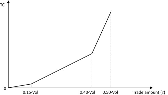
An example of a piecewise-linear function of transaction costs for a trade of size t of a particular security is illustrated in Figure 1. The transaction cost function in the graph assumes that the rate of increase of transaction costs (reflected in the slope of the function) changes at certain threshold points. For example, it is smaller in the range 0 to 15% of daily volume than in the range 15% to 40% of daily volume (or some other trading volume index). Mathematically, the transaction cost function in Figure 1 can be expressed as

where s1, s2, s3 are the slopes of the three linear segments on the graph. (They are given data.)

To include piecewise-linear functions for transaction costs in the objective function of a mean-variance (or any general mean-risk) portfolio optimization problem, we need to introduce new decision variables that correspond to the number of pieces in the piecewise-linear approximation of the transaction cost function (in this case, there are three linear segments, so we introduce variables z1, z2, z3). We write the penalty term in the objective function for an individual stock as8

If there are N stocks in the portfolio, the total transaction cost will be the sum of the transaction costs for each individual stock, that is, the penalty term that involves transaction costs in the objective function becomes

In addition, we specify the following constraints on the new decision variables:

Note that because of the increasing slopes of the linear segments and the goal of making that term as small as possible in the objective function, the optimizer will never set the decision variable corresponding to the second segment, z2,i, to a number greater than 0 unless the decision variable corresponding to the first segment, z1,i, is at its upper bound. Similarly, the optimizer would never set z3,i to a number greater than 0 unless both z1,i and z2,i are at their upper bounds. So, this set of constraints allows us to compute the amount of transaction costs incurred in the trading of stock i as z1,i+z2,i+z3,i.

Of course, we also need to link the amount of transaction costs incurred in the trading of stock i to the optimal portfolio allocation. This can be done by adding a few more variables and constraints. We introduce variables yi, one for each stock in the portfolio, that would represent the amount traded (but not the direction of the trade) and would be nonnegative. Then, we require that

and also that yi equals the change in the portfolio position of stock i. The latter condition can be imposed by writing the constraint

where w0,i and wi are the initial and the final amount of stock i in the portfolio, respectively.9

Despite their apparent complexity, piecewise-linear approximations for transaction costs are very solver-friendly, and save time (relative to nonlinear models) in the actual portfolio optimization. Although modeling transaction costs this way requires introducing new decision variables and constraints, the increase in the dimension of the portfolio optimization problem does not affect significantly the running time or the performance of the optimization solver, because the problem formulation is easy from a computational perspective.

Quadratic Transaction Costs

The transaction cost function is often parameterized as a quadratic function of the form

The coefficients ci and di are calibrated from data--for example, by fitting a quadratic function to an observed pattern of transaction costs realized for trading a particular stock under normal conditions.

Including this function in the objective function of the portfolio optimization problem results in a quadratic program that can be solved with widely available quadratic optimization software.

Fixed Transaction Costs

In some cases, we need to model fixed transaction costs. Those are costs that are incurred independently of the amount traded. To include such costs in the portfolio optimization problem, we need to introduce binary variables δ1, … , δN corresponding to each stock, where δi equals 0 if the amount traded of stock i is 0, and 1 otherwise. The idea is similar to the idea we used to model the requirement that only a given number of stocks can be included in the portfolio.

Suppose the fixed transaction cost is ai for stock i. Then, the transaction cost function is

The objective function formulation is then

and we need to add the following constraints to make sure that the binary variables are linked to the trades | wi – w0,i |:

where M is a “large” constant. When the trading size | wi – w0,i | is nonzero, δi will be forced to be 1. When the trading size is 0, then δi can be either 0 or 1, but the optimizer will set it to 0, since it will try to make its value the minimum possible in the objective function.

Of course, combinations of different trading cost models can be used in practice. For example, if the trade involves both a fixed and a variable quadratic transaction cost, then we could use a transaction cost function of the kind

The important takeaway from this section is that when transaction costs are included in the portfolio rebalancing problem, the result is a reduced amount of trading and rebalancing, and a different portfolio allocation than the one that would be obtained if transaction costs are not taken into consideration.

INCORPORATING TAXES

When stocks in a portfolio appreciate or depreciate in value, capital gains (respectively, losses) accumulate. When stocks are sold, investors pay taxes on the realized net capital gains. The taxes are computed as a percentage of the difference between the current market value of the stocks and their tax basis, where the tax basis is the price at which the stocks were bought originally.10 The percentage is less for long-term capital gains (when stocks have been held for more than a year) than it is for short-term capital gains (when stocks have been held for less than a year).11 Since shares of the same stock could have been bought at different points in time (in different lots), selling one lot of the stock as opposed to another could incur a different amount of tax. In addition to capital gains taxes, investors who are not exempt from taxes owe taxes on the dividends paid on stocks in their portfolios. Those dividends are historically taxed at a higher rate than capital gains, and may eventually be taxed as income, that is, at the investor’s personal tax rate. The tax liability of a particular portfolio therefore depends on the timing of the execution of trades, on the tax basis of the portfolio, on the accumulated short-term and long-term capital gains, and on the tax bracket of the investor.

Over two-thirds of marketable portfolio assets in the United States are held by individuals, insurance, and holding companies who pay taxes on their returns. (Exceptions are, for example, pension funds, which do not pay taxes year-to-year.) Studies have indicated that taxes are the greatest expense investors face—greater than commissions and investment management fees. To gain some intuition about the effect of taxes on the income of an investor over the investor’s lifetime, consider a portfolio that has a capital appreciation of 6.00% per year. After 30 years, $1,000 invested in that portfolio will turn into $1,000 · (1 + 0.06)30 = $5,743.49. Now suppose that the capital gains are realized each year, and a tax of 35% is paid on the gains (the remainder is reinvested). After 30 years, $1,000 invested in the portfolio will turn into $1,000 · (1 + (1 − 0.35) · 0.06)30 = $3,151.13, about half of the amount without taxes even when the tax is about one third of the capital gains. In fact, in order to provide the same return as the portfolio with no taxes, the portfolio with annual realized capital gains would need to generate a capital appreciation of 9.23% per year! One can imagine that the same logic would make benchmark tracking and performance measurement very difficult on an after-tax basis.

As investors have become more aware of the dramatic impact of taxes on their returns, there is increasing pressure on portfolio managers to include tax considerations in their portfolio rebalancing decisions and to report after-tax performance. Consequently, the demand for computationally efficient and quantitatively rigorous methods for taking taxes into consideration in portfolio allocation decisions has grown in recent years. The complexity of the problem of incorporating taxes, however, is considerable, both from a theoretical and practical perspective:

We need to emphasize that while many of the techniques described in the previous sections of this entry are widely known, there are no standard practices for tax-aware portfolio management that appear to be established. Different asset management firms interpret tax-aware portfolio allocation and approach the problem differently. To some firms, minimizing turnover,13 for example, by investing in index funds, or selecting strategies that minimize the portfolio dividend yield,14 qualify as tax-aware portfolio strategies. Other asset management firms employ complex optimization algorithms that incorporate tax considerations directly in portfolio rebalancing decisions, so that they can keep up with the considerable burden of keeping track of thousands of managed accounts and their tax preferences. The fact is, even using simple rules of thumb, such as always selling stocks from the oldest lots after rebalancing the portfolio with classical portfolio optimization routines, can have a positive effect on after-tax portfolio returns. The latter strategy minimizes the likelihood that short-term gains will be incurred, which in turn reduces taxes, because short-term capital gains are taxed at a higher rate than long-term capital gains.

Apelfeld, Fowler, and Gordon (1996) suggest a tax-aware portfolio rebalancing framework that incorporates taxes directly into the portfolio optimization process. The main idea of the approach is to treat different lots of the same stock as different securities, and then penalize for taxes as if they were different transaction costs associated with the sale of each lot. (This means, for example, that Microsoft stock bought on Date 1 is treated as a different security from Microsoft stock bought on Date 2.) Many tax-aware quantitative investment strategies employ versions of this approach, but there are a few issues to beware of when using it in practice:

• The first one is a general problem for all tax-aware approaches when they are used in the context of active portfolio management. For a portfolio manager who handles thousands of different accounts with different tax exposures, it is virtually impossible to pay attention to the tax cost incurred by each individual investor. While the tax-aware method described above minimizes the overall tax burden by reducing the amount of realized short-term sales, it has no provisions for differentiating between investors in different tax brackets because it is difficult to think of each trade as divided between all investors, and adjusted for each individual investor’s tax circumstances. This issue is so intractable that in practice it is not really brought under consideration.
• The dimension of the problem can become unmanageable very quickly. For example, a portfolio of 1,000 securities, each of which has 10 different lots, is equivalent to a portfolio of 10,000 securities when each lot is treated as a different security. Every time a new purchase is realized, a new security is added to the portfolio, since a new lot is created. One needs to exercise care and “clean up” lots that have been sold and therefore have holdings of zero each time the portfolio is rebalanced.
• Practitioners typically use factor models for forecasting returns and estimating risk. One of the assumptions when measuring portfolio risk through factor models is that the specific risk of a particular security is uncorrelated with the specific risk of other securities. (The only risk they share is the risk expressed through the factors in the factor model.) This assumption clearly does not hold when different “securities” are in fact different lots of the same stock.

DiBartolomeo (2000) describes a modification to the model used by Northfield Information Service’s portfolio management software that eliminates the last two problems. Instead of treating each lot as a separate security, the software imposes piecewise-linear transaction costs (see Figure 1) where the break points on the horizontal axis correspond to the current size of different lots of the same security. The portfolio rebalancing algorithm goes through several iterations for the portfolio weights, and at each iteration, only the shares in the highest cost basis tax lot can be traded. Other shares of the same stock can be traded in subsequent iterations of the algorithm, with their appropriate tax costs attached.

The approaches we described so far take into consideration the short-term or long-term nature of capital gains, but do not incorporate the ability to offset capital gains and losses accumulated over the year. This is an inherent limitation of single-period portfolio rebalancing approaches and is a strong argument in favor of adopting more realistic multiperiod portfolio optimization approaches. The rebalancing of the portfolio at each point in time should be made not only by considering the immediate consequences for the market value of the portfolio, but also the opportunity to correct for tax liabilities by realizing other capital gains or losses by the end of the taxable year. The scarce theoretical literature on multiperiod tax-aware portfolio optimization contains some characterizations of optimal portfolio strategies under numerous simplifying assumptions.15 However, even under such simplifying assumptions, the dimension of the problem grows exponentially with the number of stocks in a portfolio, and it is difficult to come up with computationally viable algorithms for portfolios of realistic size.

MULTIACCOUNT OPTIMIZATION

Portfolio managers who handle multiple accounts face an important practical issue. When individual clients’ portfolios are managed, portfolio managers incorporate their clients’ preferences and constraints. However, on any given trading day, the necessary trades for multiple diverse accounts are pooled and executed simultaneously. Moreover, typically trades may not be crossed, that is, it is not simply permissible to transfer an asset that should be sold on behalf of one client into the account of another client for whom the asset should be bought.16 The trades should be executed in the market. Thus, each client’s trades implicitly impact the results for the other clients: The market impact of the combined trades may be such that the benefits sought for individual accounts through trading are lost due to increased overall transaction costs. A robust multiaccount management process should ensure accurate accounting and fair distribution of transaction costs among the individual accounts.

One possibility to handle the effect of trading in multiple accounts is to use an iterative process, in which at each iteration the market impact of the trades in previous iterations is taken into account.17 More precisely, single clients’ accounts are optimized as usual, and once the optimal allocations are obtained, the portfolio manager aggregates the trades and computes the actual marginal transaction costs based on the aggregate level of trading. The portfolio manager then reoptimizes individual accounts using these marginal transaction costs, and aggregates the resulting trades again to compute new marginal transaction costs, and so on. The advantage of this approach is that little needs to be changed in the way individual accounts are typically handled, so the existing single-account optimization and management infrastructure can be reused. The disadvantage is that most generally, this iterative approach does not guarantee a convergence (or its convergence may be slow) to a “fair equilibrium,” in which clients’ portfolios receive an unbiased treatment with respect to the size and the constraint structure of their accounts.18 The latter equilibrium is the one that would be attained if all clients traded independently and competitively in the market for liquidity, and it is thus the correct and fair solution to the aggregate trading problem.

An alternative, more comprehensive approach is to optimize trades across all accounts simultaneously. O’Cinneide, Scherer, and Xu (2006) describe such a model and show that it attains the fair equilibrium we mentioned above.19 Assume that client k’s utility function is given by uk and is in the form of a dollar return penalized for risk. Assume also that a transaction cost model τ gives the cost of trading in dollars, and that τ is a convex increasing function.20 Its exact form will depend on the details of how trading is implemented. Let t be the vector of trades. It will typically have the form , that is, it will specify the aggregate buys t+i and the aggregate sells t−i for each asset i=1, … , N, but it may also incorporate information about how the trade could be carried out.21

The multiaccount optimization problem can be formulated as

where wk is the N-dimensional vector of asset holdings (or weights) of client k, and Ck is the collection of constraints on the portfolio structure of client k. The objective can be interpreted as maximization of net expected utility, that is, as maximization of the expected dollar return penalized for risk and net of transaction costs.

The problem can be simplified by making some reasonable assumptions. For example, it can be assumed that the transaction cost function τ is additive across different assets, that is, that trades in one asset do not influence trading costs in another. In such a case, the trading cost function can be split into more manageable terms, that is,

where is the cost of trading asset i as a function of the aggregate buys and sells of that asset. Splitting the terms further into separate costs of buying and selling, however, is not a reasonable assumption, because simultaneous buying and selling of an asset tends to have an offsetting effect on its price.

To formulate the problem completely, let w0k be the vector of original holdings (or weights) of client k’s portfolio, wk be the vector of decision variables for the optimal holdings (or weights) of client k’s portfolio, and be constants that convert the holdings (or weight) of each asset i in client i’s portfolio wk,i to dollars, that is, is client k’s dollar holdings of asset i.22 We also introduce new variables w+k to represent the an upper bound on the weight of each asset client k will buy:

The aggregate amount of asset i bought for all clients can then be computed as

The aggregate amount of asset i sold for all clients can be easily expressed by noticing that the difference between the amounts bought and sold of each asset are exactly equal to the total amount of trades needed to get from the original position w0k,i to the final position wk,i of that asset:23

Here t+i and t−i are nonnegative variables.

The multiaccount optimization problem then takes the form

O’Cinneide, Scherer, and Xu (2006) studied the behavior of the model in simulated experiments with a simple model for the transaction cost function, namely, one in which

where t is the trade size, and θ and γ are constants satisfying θ ≥ 0 and γ ≥ 1.24 θ and γ are specified in advance and calibrated to fit observed trading costs in the market. The transaction costs for each client k can therefore be expressed as

O’Cinneide, Scherer, and Xu (2006) observed that key portfolio performance measures, such as the information ratio (IR),25 turnover, and total transaction costs, change under this model relative to the traditional approach. Not surprisingly, the turnover and the net information ratios of the portfolios obtained with multiaccount optimization are lower than those obtained with single-account optimization under the assumption that accounts are traded separately, while transaction costs are higher. These results are in fact more realistic, and they are a better representation of the postoptimization performance of multiple client accounts in practice.

ROBUST PARAMETER ESTIMATION

The most commonly used approach for estimating security expected returns, covariances, and other parameters that are inputs to portfolio optimization models is to calculate the sample analogues from historical data. These are sample estimates for the parameters we need. It is important to remember that when we rely on historical data for estimation purposes, we in fact assume that the past provides a good representation of the future.

It is well known, however, that expected returns exhibit significant time variation (referred to as nonstationarity). They are impacted by changes in markets and economic conditions, such as interest rates, the political environment, consumer confidence, and the business cycles of different industry sectors and geographical regions. Consequently, extrapolated historical returns are often poor forecasts of future returns.

Similarly, the covariance matrix is unstable over time. Moreover, sample estimates of covariances for portfolios with thousands of stocks are notoriously unreliable, because we need large data sets to estimate them, and such large data sets of relevant data are difficult to procure. Estimates of the covariance matrix based on factor models are often used to reduce the number of statistical estimates needed from a limited set of data.

In practice, portfolio managers often alter historical estimates of different parameters subjectively or objectively, based on their expectations and forecasting models for future trends. They also use statistical methods for finding estimators that are less sensitive to outliers and other sampling errors, such as Bayesian and shrinkage estimators. A complete review of advanced statistical estimation topics is beyond the scope of this entry. We provide a brief overview of the most widely used concepts.26

Shrinkage is a form of averaging different estimators. The shrinkage estimator typically consists of three components: (1) an estimator with little or no structure (like the sample mean); (2) an estimator with a lot of structure (the shrinkage target); and (3) a coefficient that reflects the shrinkage intensity. Probably the most well-known estimator for expected returns in the financial literature was proposed by Jorion (1986). The shrinkage target in Jorion’s model is a vector array with the return on the minimum variance portfolio, and the shrinkage intensity is determined from a specific formula.27 Shrinkage estimators are used for estimates of the covariance matrix of returns as well,28 although equally weighted portfolios of covariance matrix estimators have been shown to be equally effective as shrinkage estimators.29

Bayesian estimation approaches, named after the English mathematician Thomas Bayes, are based on subjective interpretations of the probability that a particular event will occur. A probability distribution, called the prior distribution, is used to represent the investor’s knowledge about the probability before any data are observed. After more information is gathered (e.g., data are observed), a formula (known as Bayes’ rule) is used to compute the new probability distribution, called the posterior distribution.

In the portfolio parameter estimation context, a posterior distribution of expected returns is derived by combining the forecast from the empirical data with a prior distribution. One of the most well-known examples of the application of the Bayesian framework in this context is the Black-Litterman model,30 which produces an estimate of future expected returns by combining the market equilibrium returns (i.e., returns that are derived from pricing models and observable data) with the investor’s subjective views. The investor’s views are expressed as absolute or relative deviations from the equilibrium together with confidence levels of the views (as measured by the standard deviation of the views).

The ability to incorporate exogenous insight, such as a portfolio manager’s opinion, into quantitative forecasting models is important; this insight may be the most valuable input to the model. The Bayesian framework provides a mechanism for forecasting systems to use both important traditional information sources such as proprietary market data and subjective external information sources such as analyst’s forecasts.

It is important to realize that regardless of how sophisticated the estimation and forecasting methods are, they are always subject to estimation error. What makes matters worse, however, is that different estimation errors can accumulate over the different activities of the portfolio management process, resulting in large aggregate errors at the final stage. It is therefore critical that the inputs evaluated at each stage are reliable and robust, so that the aggregate impact of estimation errors is minimized.

PORTFOLIO RESAMPLING

Robust parameter estimation is only one part of ensuring that the quantitative portfolio management process as a whole is reliable. It has been observed that portfolio allocation schemes are very sensitive to small changes in the inputs that go into the optimizer. In particular, a well-known study by Black and Litterman31 demonstrated that in the case of mean-variance optimization, small changes in the inputs for expected returns had a substantial impact on the portfolio composition. “Optimal” portfolios constructed under conditions of uncertainty can have extreme or nonintuitive weights for some stocks.

With advances in computational capabilities and new research in the area of optimization under uncertainty, practitioners in recent years have been able to incorporate considerations for uncertainty not only at the estimation, but also at the portfolio optimization stage. Methods for taking into consideration inaccuracies in the inputs to the portfolio optimization problem include simulation (resampling) and robust optimization. We explain portfolio resampling in this section, and robust portfolio optimization in the following section.

A logical approach to making portfolio allocation more robust with respect to changes in the input parameters is to generate different scenarios for the values these parameters can take, and to find weights that remain stable for small changes in the input parameters. This method is referred to as portfolio resampling.32 To illustrate the resampling technique, we explain how it is applied to portfolio mean-variance optimization.

Suppose that we have initial estimates for the expected stock returns, , and covariance matrix, , for the N stocks in the portfolio. (We use “hat” to denote a statistical estimate.)

1. We simulate S samples of N returns from a multivariate normal distribution with mean and covariance matrix .

2. We use the S samples generated in (1) to compute S new estimates of vectors of expected returns and covariance matrices .

3. We solve S portfolio optimization problems, one for each estimated pair of expected returns and covariances (,), and save the weights for the N stocks in a vector array w(s), where s = 1, … , S. (The optimization problem itself could be any of the standard mean-variance formulations: maximize expected return subject to constraints on risk, minimize risk subject to constraints on the expected return, or maximize the utility function.)

4. To find the final portfolio weights, we average out the weight for each stock over the S weights found for that stock in each of the S optimization problems. In other words,

For example, stock i in the portfolio has final weight

5. Perhaps even more valuable than the average estimate of the weights obtained from the simulation and optimization iterations is the probability distribution we obtain for the portfolio weights. If we plot the weights for each stock obtained over the S iterations, , we can get a sense for how variable this stock weight is in the portfolio. A large standard deviation computed from the distribution of portfolio weight i will be an indication that the original portfolio weight was not very precise due to estimation error.

An important question, of course, is how large is “large enough.” Do we have evidence that the portfolios we obtained through resampling are statistically different from one another? We can evaluate that by using a test statistic. For example, it can be shown that the test statistic

follows a chi-square (χ2) distribution with degrees of freedom equal to the number of securities in the portfolio. If the value of this statistic is statistically “large,” then there will be evidence that the portfolio weights w* and w are statistically different. This is an important insight for the portfolio manager, and its applications extend beyond just resampling. Let us provide some intuition as to why.

Suppose that we are considering rebalancing our current portfolio. Given our forecasts of expected returns and risk, we could calculate a set of new portfolios through the resampling procedure. Using the test statistic above, we determine whether the new set of portfolio weights is statistically different from our current weights and, therefore, whether it would be worthwhile to rebalance or not. If we decide that it is worthwhile to rebalance, we could choose any of the resampled portfolios that are statistically different from our current portfolio. Which one should we choose? A natural choice would be to select the portfolio that would lead to the lowest transaction costs. The idea of determining statistically equivalent portfolios, therefore, has much wider implications than the ones illustrated in the context of resampling.

Resampling has its drawbacks:

• Since the resampled portfolio is calculated through a simulation procedure in which a portfolio optimization problem needs to be solved at each step, the approach is computationally cumbersome, especially for large portfolios. There is a trade-off between the number of resampling steps and the accuracy of estimation of the effect of errors on the portfolio composition.
• Due to the averaging in the calculation of the final portfolio weights, it is highly likely that all stocks will end up with nonzero weights. This has implications for the amount of transaction costs that will be incurred if the final portfolio is to be attained. One possibility is to include constraints that limit both the turnover and the number of stocks with nonzero weights. As we saw earlier, however, the formulation of such constraints adds another level of complexity to the optimization problem and will slow down the resampling procedure.
• Since the averaging process happens after the optimization problems are solved, the final weights may not actually satisfy some of the constraints in the optimization formulation. In general, only convex (such as linear) constraints are guaranteed to be satisfied by the averaged final weights. Turnover constraints, for example, may not be satisfied. This is a serious limitation of the resampling approach for practical applications.

Despite these limitations, resampling has advantages and presents a good alternative to using only point estimates of inputs to the optimization problem.

ROBUST PORTFOLIO OPTIMIZATION

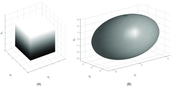
Another way in which uncertainty about the inputs can be modeled is by incorporating it directly into the optimization process. Robust optimization is an intuitive and efficient way to deal with uncertainty. Robust portfolio optimization does not use the traditional forecasts, such as expected returns and covariances, but rather uncertainty sets containing these point estimates. An example of such an uncertainty set is a confidence interval around the forecast for each expected return (“alpha”). This uncertainty shape looks like a “box” in the space of the input parameters. (See Figure 2(A).) We can also formulate advanced uncertainty sets that incorporate more knowledge about the estimation error. For instance, a widely used uncertainty set is the ellipsoidal uncertainty set, which takes into consideration the covariance structure of the estimation errors. (See Figure 2(B).) We will see examples of both uncertainty sets in this section.

Figure 2 (A) Box Uncertainty Set in Three Dimensions; (B) Ellipsoidal Uncertainty Set in Three Dimensions

The robust optimization procedure for portfolio allocation is as follows. First, we specify the uncertainty sets around the input parameters in the problem. Then, we ask what the optimal portfolio allocation is when the input parameters take the worst possible value inside these uncertainty sets. In effect, we solve an inner problem that determines the worst possible realization of the uncertain parameters over the uncertainty set before we solve the original problem of optimal portfolio allocation.

Let us give a specific example of how the robust optimization framework can be applied in the portfolio optimization context. Consider the utility function formulation of the mean-variance portfolio allocation problem:

Suppose that we have estimates and of the vector of expected returns and the covariance matrix. Instead of the estimate , however, we will consider a set of vectors that are “close” to . We define the box uncertainty set

In words, the set contains all vectors such that each component is in the interval . We then solve the following problem:

This is called the robust counterpart of the original problem. It is a max-min problem that searches for the optimal portfolio weights when the estimates of the uncertain returns take their worst-case values within the prespecified uncertainty set in the sense that the value of the objective function is the worst it can be over all possible values for the expected returns in the uncertainty set.

It can be shown33 that the max-min problem above is equivalent to the following problem

where |w| denotes the absolute value of the entries of the vector of weights w. To gain some intuition, notice that if the weight of stock i in the portfolio is negative, the worst-case expected return for stock i is (we lose the largest amount possible). If the weight of stock i in the portfolio is positive, then the worst-case expected return for stock i is (we gain the smallest amount possible). Observe that equals if the weight wi is positive and if the weight wi is negative. Hence, the mathematical expression in the objective agrees with our intuition: It minimizes the worst-case expected portfolio return. In this robust version of the mean-variance formulation, stocks whose mean return estimates are less accurate (i.e., have a larger estimation error ) are therefore penalized in the objective function and will tend to have a smaller weight in the optimal portfolio allocation.

This optimization problem has the same computational complexity as the nonrobust mean-variance formulation—namely, it can be stated as a quadratic optimization problem. The latter can be achieved by using a standard trick that allows us to get rid of the absolute values for the weights. The idea is to introduce an N-dimensional vector of additional variables to replace the absolute values | w |, and to write an equivalent version of the optimization problem,

Therefore, incorporating considerations about the uncertainty in the estimates of the expected returns in this example has virtually no computational cost.

We can view the effect of this particular “robustification” of the mean-variance portfolio optimization formulation in two different ways. On the one hand, we can see that the values of the expected returns for the different stocks have been adjusted downward in the objective function of the optimization problem. The robust optimization model “shrinks” the expected return of stocks with large estimation error, that is, in this case the robust formulation is related to statistical shrinkage methods, which we introduced earlier in this entry. On the other hand, we can interpret the additional term in the objective function as a “risk-like” term that represents penalty for estimation error. The size of the penalty is determined by the investor’s aversion to estimation risk and is reflected in the magnitude of the deltas.

More complicated specifications for uncertainty sets have more involved mathematical representations, but can still be selected so that they preserve an easy computational structure for the robust optimization problem. For example, we can use the ellipsoidal uncertainty set from Figure 2(B), which can be expressed mathematically as

Here is the covariance matrix of estimation errors for the vector of expected returns . This uncertainty set represents the requirement that the sum of squares (scaled by the inverse of the covariance matrix of estimation errors) between all elements in the set and the point estimates can be no larger than δ2. We note that this uncertainty set cannot be interpreted as individual confidence intervals around each point estimate. Instead, it captures the idea of a joint confidence region. In practical applications, the covariance matrix of estimation errors is often assumed to be diagonal. In the latter case, the set contains all vectors of expected returns that are within a certain number of standard deviations from the point estimate of the vector of expected returns, and the resulting robust portfolio optimization problem would protect the investor if the vector of expected returns is within that range.

It can be shown that the robust counterpart of the mean-variance portfolio optimization problem with an ellipsoidal uncertainty set for the expected return estimates is the following optimization problem formulation:

This is a second-order cone optimization problem and requires specialized software to solve, but the methods for solving it are very efficient.

Similarly to the case of the robust counterpart with a box uncertainty set, we can interpret the extra term in the objective function () as the penalty for estimation risk, where δ incorporates the degree of the investor’s aversion to estimation risk. Note, by the way, that the covariance matrix in the estimation error penalty term, , is not necessarily the same as the covariance matrix of returns . In fact, it is not immediately obvious how can be estimated from data. is the covariance matrix of the errors in the estimation of the expected (average) returns. Thus, if a portfolio manager forecasts 5% active return over the next time period, but gets 1%, the manager cannot argue that there was a 4% error in the expected return—the actual error would consist of both an estimation error in the expected return and the inherent volatility in actual realized returns. In fact, critics of the approach such as Lee, Stefek, and Zhelenyak (2006) have argued that the realized returns typically have large stochastic components that dwarf the expected returns, and hence estimating from data is very hard, if not impossible.

Several approximate methods for estimating have been found to work well in practice. For example, Stubbs and Vance (2005) observe that simpler estimation approaches, such as using just the diagonal matrix containing the variances of the estimates (as opposed to the complete error covariance matrix), often provide most of the benefit in robust portfolio optimization. In addition, standard approaches for estimating expected returns, such as Bayesian statistics and regression-based methods, can produce estimates for the estimation error covariance matrix in the process of generating the estimates themselves.34

Among practitioners, the notion of robust portfolio optimization is often equated with the robust mean-variance model we discussed in this section, with the box or the ellipsoidal uncertainty sets for the expected stock returns. While robust optimization applications often involve one form or another of this model, the actual scope of robust optimization can be much broader. We note that the term robust optimization refers to the technique of incorporating information about uncertainty sets for the parameters in the optimization model, and not to the specific definitions of uncertainty sets or the choice of parameters to model as uncertain. For example, we can use the robust optimization methodology to incorporate considerations for uncertainty in the estimate of the covariance matrix in addition to the uncertainty in expected returns, and obtain a different robust portfolio allocation formulation. Robust optimization can be applied also to portfolio allocation models that are different from the mean-variance framework, such as Sharpe ratio optimization and value-at-risk optimization.35 Finally, robust optimization has the potential to provide a computationally efficient way to handle portfolio optimization over multiple stages—a problem for which so far there have been few satisfactory solutions.36 There are numerous useful robust formulations, but a complete review is beyond the scope of this entry.37

Is implementing robust optimization formulations worthwhile? Some tests with simulated and real market data indicate that robust optimization, when inaccuracy is assumed in the expected return estimates, outperforms classical mean-variance optimization in terms of total excess return a large percentage (70–80%) of the time (see, for example, Ceria and Stubbs, 2006). Other tests have not been as conclusive (see, for example, Lee, Stefek, and Zhelenyak, 2006). The factor that accounts for much of the difference is how the uncertainty in parameters is modeled. Therefore, finding a suitable degree of robustness and appropriate definitions of uncertainty sets can have a significant impact on portfolio performance.

Independent tests by practitioners and academics using both simulated and market data appear to confirm that robust optimization generally results in more stable portfolio weights, that is, that it eliminates the extreme corner solutions resulting from traditional mean-variance optimization. This fact has implications for portfolio rebalancing in the presence of transaction costs and taxes, as transaction costs and taxes can add substantial expenses when the portfolio is rebalanced. Depending on the particular robust formulations employed, robust mean-variance optimization also appears to improve worst-case portfolio performance and results in smoother and more consistent portfolio returns. Finally, by preventing large swings in positions, robust optimization typically makes better use of the turnover budget and risk constraints.

Robust optimization, however, is not a panacea. By using robust portfolio optimization formulations, investors are likely to trade off the optimality of their portfolio allocation in cases in which nature behaves as they predicted for protection against the risk of inaccurate estimation. Therefore, investors using the technique should not expect to do better than classical portfolio optimization when estimation errors have little impact, or when typical scenarios occur. They should, however, expect insurance in scenarios in which their estimates deviate from the actual realized values by up to the amount they have prespecified in the modeling process.

KEY POINTS

• Commonly used constraints in practice include long-only (no short-selling) constraints, turnover constraints, holding constraints, risk factor constraints, and tracking error constraints. These constraints can be handled in a straightforward way by the same type of optimization algorithms used for solving the classical mean-variance portfolio allocation problem.
• Minimum holding constraints, transaction size constraints, cardinality constraints, and round-lot constraints are also widely used in practice, but their nature is such that they require binary and integer modeling, which necessitates the use of mixed-integer and other specialized optimization solvers.
• Transaction costs can easily be incorporated in standard portfolio allocation models. Typical functions for representing transaction costs include linear, piecewise linear, and quadratic.
• Taxes can have a dramatic effect on portfolio returns; however, it is difficult to incorporate them into the classical portfolio optimization framework. Their importance to the individual investor is a strong argument for taking a multiperiod view of investments, but the computational burden of multiperiod portfolio optimization formulations with taxes is extremely high.
• For investment managers who handle multiple accounts, increased transaction costs because of the market impact of simultaneous trades can be an important practical issue and should be taken into consideration when individual clients’ portfolio allocation decisions are made to ensure fairness across accounts.
• As the use of quantitative techniques has become widespread in the investment industry, the consideration of estimation risk and model risk has grown in importance. Methods for robust statistical estimation of parameters include shrinkage and Bayesian techniques.
• Portfolio resampling is a technique that uses simulation to generate multiple scenarios for possible values of the input parameters in the portfolio optimization problem and aims to determine portfolio weights that remain stable with respect to small changes in model parameters.
• Robust portfolio optimization incorporates uncertainty directly into the optimization process. The uncertain parameters in the optimization problem are assumed to vary in prespecified uncertainty sets that are selected subjectively or based on data.

NOTES

1. See Chapter 1 in Maginn and Tuttle (1990).

2. Multiperiod portfolio optimization models are still rarely used in practice, not because the value of multiperiod modeling is questioned, but because such models are often too intractable from a computational perspective.

3. As the term intuitively implies, the ADV measures the total amount of a given asset traded in a day on average, where the average is taken over a prespecified time period.

4. Another computationally tractable situation for minimizing CVaR is when the data are normally distributed. In that case, minimizing CVaR is equivalent to minimizing the standard deviation of the portfolio.

5. See Chapters 8 and 9 in Pachamanova and Fabozzi (2010) for a more detailed explanation of CVaR and a derivation of the optimization formulation.

6. Versions of this model have been suggested in Pogue (1970), Schreiner (1980), Adcock and Meade (1994), Lobo, Fazel, and Boyd (2000), and Mitchell and Braun (2004).

7. Here we are thinking of wi as the portfolio weights, but in fact it may be more intuitive to think of the transaction costs as a percentage of amount traded. It is easy to go back and forth between portfolio weights and portfolio amounts by simply multiplying wi by the total amount in the portfolio. In fact, we can switch the whole portfolio optimization formulation around and write it in terms of allocation of dollars, instead of weights. We just need to replace the vector of weights w by a vector x of dollar holdings.

8. See, for example, Bertsimas, Darnell, and Soucy (1999).

9. As we explained earlier, this constraint can be written in an equivalent, more optimization solver-friendly form, namely,

10. The computation of the tax basis is different for stocks and bonds. For bonds, there are special tax rules, and the original price is not the tax basis.

11. The exact rates vary depending on the current version of the tax code, but the main idea behind the preferential treatment of long-term gains to short-term gains is to encourage long-term capital investments and fund entrepreneurial activity.

12. See Stein (1998).

13. See Apelfeld, Fowler, and Gordon (1996) who show that a manager can outperform on an after-tax basis with high turnover as well, as long as the turnover does not result in net capital gains taxes. (There are other issues with high turnover, however, such as higher transaction costs that may result in a lower overall portfolio return.)

14. Dividends are taxed as regular income, i.e., at a higher rate than capital gains, so minimizing the portfolio dividend yield should theoretically result in a lower tax burden for the investor.

15. See Constantinides (1983), Dammon and Spatt (1996), and Dammon, Spatt, and Zhang (2001 and 2004).

16. The Securities and Exchange Commission (SEC) in general prohibits cross-trading but does provide exemptions if prior to the execution of the cross trade the asset manager can demonstrate to the SEC that a particular cross trade benefits both parties. Similarly, Section 406(b)(3) of the Employee Retirement Income Security Act of 1974 (ERISA) forbids cross-trading, but there is new cross-trading exemption in Section 408(b)(19) adopted in the Pension Protection Act of 2006.

17. Khodadadi, Tutuncu, and Zangari (2006).

18. The iterative procedure is known to converge to the equilibrium, however, under special conditions. See O’Cinneide, Scherer, and Xu (2006).

19. The issue of considering transaction costs in multiaccount optimization has been discussed by others as well. See, for example, Bertsimas, Darnell, and Soucy (1999).

20. As we mentioned earlier in this entry, realistic transaction costs are in fact described by nonlinear functions, because costs per share traded typically increase with the size of the trade due to market impact.

21. For example, if asset i is a euro-pound forward, then a trade in that asset can also be implemented as a euro-dollar forward plus a dollar-forward, so there will be two additional assets in the aggregate trade vector t.

22. Note that equals 1 if wk,i is the actual dollar holdings.

23. Note that, similarly to w+k, we could introduce additional sell variables w−k, but this is not necessary. By expressing aggregate sales through aggregate buys and total trades, we reduce the dimension of the optimization problem, because there are fewer decision variables. This would make a difference for the speed of obtaining a solution, especially in the case of large portfolios and complicated representation of transaction costs.

24. Note that γ = 1 defines linear transaction costs. For linear transaction costs, multiaccount optimization produces the same allocation as single-account optimization, because linear transaction costs assume that an increased aggregate amount of trading does not have an impact on prices.

25. The information ratio is the ratio of (annualized) portfolio residual return (alpha) to (annualized) portfolio residual risk, where risk is defined as standard deviation.

26. For further details, see Chapters 6, 7, and 8 in Fabozzi, Kolm, Pachamanova, and Focardi (2007).

27. See Chapter 8 in Fabozzi, Kolm, Pachamanova, and Focardi (2007).

28. See, for example, Ledoit and Wolf (2003).

29. For an overview of such models, see Disatnik and Benninga (2007).

30. For a step-by-step description of the Black-Litterman model, see Chapter 8 in Fabozzi, Kolm, Pachamanova, and Focardi (2007).

31. See Black and Litterman (1992).

32. See Michaud (1998), Jorion (1992), and Scherer (2002).

33. For derivation, see, for example, Chapter 12 in Fabozzi, Kolm, Pachamanova, and Focardi (2007) or Chapter 9 in Pachamanova and Fabozzi (2010).

34. For a more in-depth coverage of the topic of estimating input parameters for robust optimization formulations, see Chapter 12 in Fabozzi, Kolm, Pachamanova, and Focardi (2007).

35. See, for example, Goldfarb and Iyengar (2003) and Natarajan, Pachamanova, and Sim (2008).

36. See Ben-Tal, Margalit, and Nemirovski (2000) and Bertsimas and Pachamanova (2008).

37. For further details, see Fabozzi, Kolm, Pachamanova, and Focardi (2007).

REFERENCES

Adcock, C., and Meade, N. (1994). A simple algorithm to incorporate transaction costs in quadratic optimization. European Journal of Operational Research 79, 1: 85–94.

Apelfeld, R., Fowler, G. B., and Gordon, J. P. (1996). Tax-aware equity investing. Journal of Portfolio Management 22, 2: 18–28.

Ben-Tal, A., Margalit, T., and Nemirovski, A. (2000). Robust modeling of multi-stage portfolio problems. In H. Frenk, K. Roos, T. Terlaky, and S. Zhang (eds.), High-Performance Optimization (Dordrecht: Kluwer Academic Publishers, pp. 303–328).

Bertsimas, D., Darnell, C., and Soucy, R. (1999). Portfolio construction through mixed-integer programming at Grantham, Mayo, Van Otterloo and Company. Interfaces 29, 1: 49–66.

Bertsimas, D., and Pachamanova, D. (2008). Robust multiperiod portfolio management with transaction costs. Computers and Operations Research, special issue on Applications of Operations Research in Finance 35, 1: 3–17.

Black, F., and Litterman, R. (1992). Global portfolio optimization. Financial Analysts Journal 48, 5: 28–43.

Ceria, S., and Stubbs, R. (2006). Incorporating estimation errors into portfolio selection: Robust portfolio construction. Journal of Asset Management 7, 2: 109–127.

Constantinides, G. (1983). Capital market equilibrium with personal taxes. Econometrica 5: 611–636.

Dammon, R. M., and Spatt, C. S. (1996). The optimal trading and pricing of securities with asymmetric capital gains taxes and transaction costs. Review of Financial Studies 9, 3: 921–952.

Dammon, R. M., Spatt, C. S., and Zhang, H. H. (2001). Optimal consumption and investment with capital gains taxes. Review of Financial Studies 14, 3: 583–617.

Dammon, R. M., Spatt, C. S., and Zhang, H. H. (2004). Optimal asset location and allocation with taxable and tax-deferred investing. Journal of Finance 59, 3: 999–1037.

David, D., and Benninga, S. (2007). Shrinking the covariance matrix—simpler is better. Journal of Portfolio Management 33, 4: 56–63.

DiBartolomeo, D. (2000). Recent advances in management of taxable portfolios. Manuscript, Northfield Information Services.

Fabozzi, F. J., Kolm, P., Pachamanova, D., and Focardi, S. (2007). Robust Portfolio Optimization and Management. Hoboken, NJ: John Wiley & Sons.

Goldfarb, D., and Iyengar, G. (2003). Robust portfolio selection problems. Mathematics of Operations Research 28, 1: 1–38.

Jorion, P. (1986). Bayes-Stein estimator for portfolio analysis. Journal of Financial and Quantitative Analysis 21, 3: 279–292.

Jorion, P. (1992). Portfolio optimization in practice. Financial Analysts Journal 48, 1: 68–74.

Khodadadi, A., Tutuncu, R., and Zangari, P. (2006). Optimization and quantitative investment management. Journal of Asset Management 7, 2: 83–92.

Ledoit, O., and Wolf, M. (2003). Improved estimation of the covariance matrix of stock returns with an application to portfolio selection. Journal of Empirical Finance 10, 5: 603–621.

Lee, J-H., Stefek, D., and Zhelenyak, A. (2006). Robust portfolio optimization—a closer look. MSCI Barra Research Insights Report, June.

Lobo, M. S., Fazel, M., and Boyd, S. (2000). Portfolio optimization with linear and fixed transaction costs and bounds on risk. Annals of Operations Research.

Maginn, J. L., and Tuttle, D. L. (eds.). (1990). Managing Investment Portfolios: A Dynamic Process. New York: Warren, Gorham & Lamont, sponsored by the Institute of Chartered Financial Analysts, Second Edition.

Michaud, R. O. (1998). Efficient Asset Management: A Practical Guide to Stock Portfolio Optimization and Asset Allocation. Oxford: Oxford University Press.

Mitchell, J. E., and Braun, S. (2004). Rebalancing an investment portfolio in the presence of convex transaction costs. Technical Report, Department of Mathematical Sciences, Rensselaer Polytechnic Institute.

Natarajan, K., Pachamanova, D., and Sim, M. (2008). Incorporating asymmetric distributional information in robust value-at-risk optimization. Management Science 54, 3: 573–585.

O’Cinneide, C., Scherer, B., and Xu, X. (2006). Pooling trades in a quantitative investment process. Journal of Portfolio Management 32, 4: 33–43.

Pachamanova, D. A., and Fabozzi, F. J. (2010). Simulation and Optimization in Finance: Modeling with MATLAB, @RISK, and VBA. Hoboken, NJ: John Wiley & Sons.

Pogue, G. (1970). An extension of the Markowitz portfolio selection model to include variable transactions costs, short sales, leverage policies, and taxes. Journal of Finance 25, 5: 1005–1027.

Rockafellar, R. T., and Uryasev, S. (2002). Conditional value-at-risk for general loss distributions. Journal of Banking and Finance 26: 1443–1471.

Rockefellar, R. T., and Uryasev, S. (2000). Optimization of conditional value-at-risk. Journal of Risk 3: 21–41.

Schreiner, J. (1980). Portfolio revision: A turnover-constrained approach. Financial Management 9, 1: 67–75.

Scherer, B. (2002). Portfolio resampling: Review and critique, Financial Analysts Journal 58, 6: 98–109.

Stein, D. M. (1998). Measuring and evaluating portfolio performance after taxes. Journal of Portfolio Management 24, 2: 117–124.

Stubbs, R., and Vance, P. (2005). Computing return estimation error matrices for robust optimization. Report, Axioma.