
Working with High-Frequency Data
This entry examines high-frequency data, the particularities and opportunities they bring, and compares these data with their low-frequency counterparts, wherever appropriate. High-frequency trading (HFT) strategies by their nature use a different population of data, and the traditional methods of data analysis need to be adjusted accordingly. Specifically, this entry examines the topics of volume, time-spacing, and bid-ask-bounce inherent in the high-frequency data.
WHAT ARE HIGH-FREQUENCY DATA?
High-frequency data, also known as “tick data,” are a record of live market activity. Every time a customer, a dealer, or another entity posts a so-called limit order to buy s units of a specific security with ticker X at price q, a bid quote qtbb is logged at time tb to buy stbbunits of X. (Market orders are incorporated into tick data in a different way as discussed below.) When the newly arrived bid quote qtbb has the highest price relative to all other previously arrived bid quotes in force, qtbbbecomes known as “the best bid” available at time tb. Similarly, when a trading entity posts a limit order to sell s units of X at price q, an ask quote qtaa is logged at time ta to sell staaunits of X. If the latest qtaa is lower than all other available ask quotes for security X, qtaa becomes known as “the best ask” at time ta.
What happens to quotes from the moment they arrive largely depends on the venue where the orders are posted. Best bids and asks posted directly on an exchange will be broadcast to all exchange participants and other parties tracking quote data. In situations when the new best bid exceeds the best ask already in force on the exchange, ![]() , most exchanges will immediately “match” such quotes, executing a trade at the preexisting best ask, qtaa at time tb. Conversely, should the newly arrived best ask fall below the current best bid,
, most exchanges will immediately “match” such quotes, executing a trade at the preexisting best ask, qtaa at time tb. Conversely, should the newly arrived best ask fall below the current best bid, ![]() , the trade is executed at the preexisting best bid, qtbb at time ta.
, the trade is executed at the preexisting best bid, qtbb at time ta.
Most dark pools match bids and asks “crossing the spread,” but may not broadcast the newly arrived quotes (hence the mysterious moniker, the “dark pools”). Similarly, quotes destined for the interdealer networks may or may not be disseminated to other market participants, depending on the venue.
Market orders contribute to high-frequency data in the form of “last trade” information. Unlike a limit order that is an order to buy a specified quantity of a security at a certain price, a market order is an order to buy a specified quantity of a security at the best price available at the moment the order is “posted” on the trading venue. As such, market orders are executed immediately at the best available bid or best ask prices, with each market buy order executed at the best ask and each market sell matched with the best bid, and the transaction is recorded in the quote data as the “last trade price” and the “last trade size.”
A large market order may need to be matched with one or several best quotes, generating several “last trade” data points. For example, if the newly arrived market buy order is smaller in size than that of the best ask, the best ask quote may still remain in force on most trading venues, but the best ask size will be reduced to reflect that the portion of the best ask quote has been matched with the market order. When the size of the incoming market buy order is bigger than the size of the corresponding best ask, the market order consumes the best ask in its entirety, and then proceeds to be matched sequentially with the next available best ask until the size of the market order is fulfilled. The remaining lowest-priced ask quote becomes the best ask available on the trading venue.
Most limit and market orders are placed in so-called “lot sizes”: increments of a certain number of units, known as a lot. In foreign exchange, a standard trading lot today is US$5 million, a considerable reduction from a minimum of $25 million entertained by high-profile brokers just a few years ago. On equity exchanges, a lot can be as low as one share, but dark pools may still enforce a 100 share minimum requirement for orders. An order for the amount other than an integer increment of a lot size is called an “odd lot.”
Small limit and market “odd lot” orders posted through a broker-dealer may be aggregated, or “packaged,” by the broker-dealer into larger-size orders in order to obtain volume discounts at the orders’ execution venue. In the process, the brokers may “sit” on quotes without transmitting them to an executing venue, delaying execution of customers’ orders.
HOW ARE HIGH-FREQUENCY DATA RECORDED?
The highest-frequency data are a collection of sequential “ticks,” arrivals of the latest quote, trade, price, order size, and volume information. Tick data usually have the following properties:
- A timestamp
- A financial security identification code
- An indicator of what information it carries
- Bid price
- Ask price
- Available bid size
- Available ask size
- Last trade price
- Last trade size
- Security-specific data, such as implied volatility for options
- The market value information, such as the actual numerical value of the price, available volume, or size
A timestamp records the date and time at which the quote originated. It may be the time at which the exchange or the broker-dealer released the quote, or the time when the trading system has received the quote. At the time this entry is written, the standard “round-trip” travel time of an order quote from the ordering customer to the exchange and back to the customer with the acknowledgement of order receipt is 15 milliseconds or less in New York. Brokers have been known to be fired by their customers if they are unable to process orders at this now standard speed. Sophisticated quotation systems, therefore, include milliseconds and even microseconds as part of their timestamps.
Another part of the quote is an identifier of the financial security. In equities, the identification code can be a ticker, or, for tickers simultaneously traded on multiple exchanges, a ticker followed by the exchange symbol. For futures, the identification code can consist of the underlying security, futures expiration date, and exchange code.
The last trade price shows the price at which the last trade in the security cleared. Last trade price can differ from the bid and ask. The differences can arise when a customer posts a favorable limit order that is immediately matched by the broker without broadcasting the customer’s quote. Last trade size shows the actual size of the last executed trade.
The best bid is the highest price available for sale of the security in the market. The best ask is the lowest price entered for buying the security at any particular time. In addition to the best bid and best ask, quotation systems may disseminate “market depth” information: the bid and ask quotes entered posted on the trading venue at prices worse than the best bid and ask, as well as aggregate order sizes corresponding to each bid and ask recorded on the trading venue’s “books.” Market depth information is sometimes referred to as the Level II data and may be disseminated as the premium subscription service only. In contrast, the best bid, best ask, last trade price, and size information (“Level I data”) is often available for a small nominal fee.
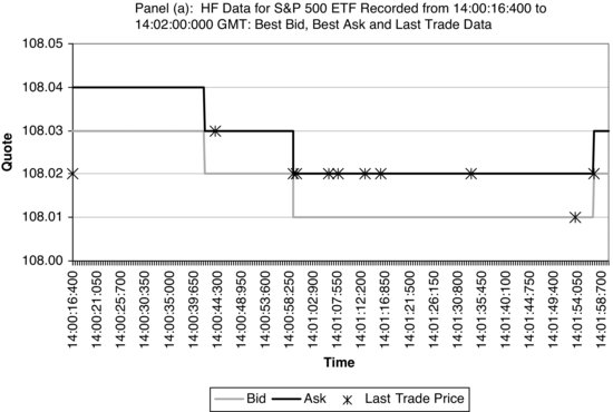
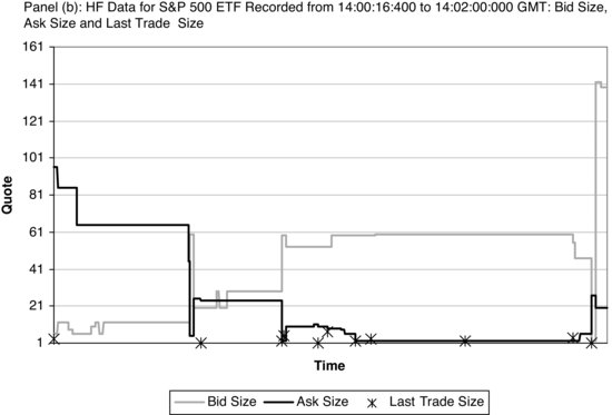
Panels (a) and (b) of Figure 1 illustrate a 30-second log of Level I high-frequency data recorded by NYSE Arca for SPDR S&P 500 ETF (ticker SPY) from 14:00:16:400 to 14:02:00:000 GMT on November 9, 2009. Panel (a) shows quote data: best bid, best ask, and last trade information, while panel (b) displays corresponding position sizes (best bid size, best ask size, and last trade size).
Figure 1 Level I High-Frequency Data Recorded by NYSE Arca for SPDR S&P 500 ETF (ticker SPY) from 14:00:16:400 to 14:02:00:000 GMT on November 9, 2009
PROPERTIES OF HIGH-FREQUENCY DATA
High-frequency securities data have been studied for many years. Yet, the concept is still something of a novelty to many academics and practitioners. Unlike daily or monthly data sets commonly used in much of financial research and related applications, high-frequency data have distinct properties, which simultaneously can be advantageous and intimidating to researchers. Table 1 summarizes the properties of high-frequency data. Each property, its advantages, and its disadvantages are discussed in detail later in the entry.
Table 1 Summary of Properties of High-Frequency Data
HIGH-FREQUENCY DATA ARE VOLUMINOUS
The nearly two-minute sample of tick data for SPDR S&P 500 ETF (ticker SPY) shown in Figure 1 contained over 100 observations of Level I data: best bid quotes and sizes, best ask quotes and sizes, and last trade prices and sizes. Table 2 summarizes the breakdown of the data points provided by NYSE Arca for SPY from 14:00:16:400 to 14:02:00:000 GMT on November 9, 2009, and SPY, Japanese yen futures, and a euro call option throughout the day on November 9, 2009. Other Level I data omitted from Table 2 include cumulative daily trade volume for SPY and Japanese yen futures, and “Greeks” for the euro call option. The number of quotes observed on November 9, 2009, for SPY alone would comprise over 160 years of daily open, high, low, close, and volume data points, assuming an average of 252 trading days per year.
Table 2 Summary Statistics for Level I Quotes for Selected Securities on November 9, 2009

The quality of data does not always match its quantity. Centralized exchanges generally provide accurate data on bids, asks, and volume of any. The information on the limit order book is less commonly available. In decentralized markets, such as foreign exchange and the interbank money market, no market-wide quotes are available at any given time. In such markets, participants are aware of the current price levels, but each institution quotes its own prices adjusted for its order book. In decentralized markets, each dealer provides his or her own tick data to clients. As a result, a specific quote on a given financial instrument at any given time may vary from dealer to dealer. Reuters, Telerate, and Knight Ridder, among others, collect quotes from different dealers and disseminate them back, improving the efficiency of the decentralized markets.
There are generally thought to be three anomalies in interdealer quote discrepancies. First, each dealer’s quotes reflect that dealer’s own inventory. For example, a dealer that has just sold a customer $100 million of USD/CAD would be eager to diversify the risk of the position and avoid selling any more of USD/CAD. Most dealers are, however, obligated to transact with their clients on tradable quotes. To incite clients to place sell orders on USD/CAD, the dealer temporarily raises the bid quote on USD/CAD. At the same time, to encourage clients to withhold placing buy orders, the dealer raises the ask quote on USD/CAD. Thus, dealers tend to raise both bid and ask prices whenever they are short in a particular financial instrument and lower both bid and ask prices whenever they are disproportionally long in a financial instrument.
Figure 2 Average Hourly Bid-Ask Spread on EUR/USD Spot for the Last Two Weeks of October 2008 on a Median Transaction Size of USD 5 million
Source: Aldridge (2009).

Second, in an anonymous marketplace, such as a dark pool, dealers as well as other market makers may “fish” for market information by sending indicative quotes that are much off the previously quoted price to assess the available demand or supply.
Third, Dacorogna et al. (2001) note that some dealers’ quotes may lag real market prices. The lag is thought to vary from milliseconds to a minute. Some dealers quote moving averages of quotes of other dealers. The dealers who provide delayed quotes usually do so to advertise their market presence in the data feed. This was particularly true when most order prices were negotiated over the telephone, allowing a considerable delay between quotes and orders. Fast-paced electronic markets discourage lagged quotes, improving the quality of markets.
Figure 3 Comparison of Average Bid-Ask Spreads for Different Hours of the Day during Normal Market Conditions and Crisis Conditions
HIGH-FREQUENCY DATA ARE SUBJECT TO BID-ASK BOUNCE
In addition to trade price and volume data long available in low-frequency formats, high-frequency data comprise bid and ask quotes and the associated order sizes. Bid and ask data arrive asynchronously and introduce noise in the quote process.
The difference between the bid quote and the ask quote at any given time is known as the bid-ask spread. The bid-ask spread is the cost of instantaneously buying and selling the security. The higher the bid-ask spread, the higher a gain the security must produce in order to cover the spread along with other transaction costs. Most low-frequency price changes are large enough to make the bid-ask spread negligible in comparison. In tick data, on the other hand, incremental price changes can be comparable or smaller than the bid-ask spread.
Bid-ask spreads usually vary throughout the day. Figure 2 illustrates the average bid-ask spread cycles observed in the institutional EUR/USD market for the last two weeks of October 2008. As Figure 2 shows, the average spread increases significantly during Tokyo trading hours when the market is quiet. The spread then reaches its lowest levels during the overlap of the London and New York trading sessions when the market has many active buyers and sellers. The spike in the spread over the weekend of October 18–19, 2008, reflects the market concern over the subpoenas issued on October 17, 2009, to senior Lehman executives in a case relating to potential securities fraud at Lehman Brothers.
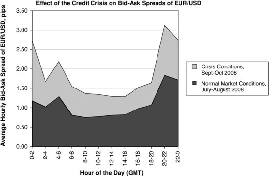
Bid-ask spreads typically increase during periods of market uncertainty or instability. Figure 3, for example, compares average bid-ask spreads on EUR/USD in the stable market conditions of July–August 2008 and the crisis conditions of September–October 2008. As the figure shows, the intraday spread pattern is persistent in both crisis and normal market conditions, but the spreads are significantly higher during crisis months than during normal conditions at all hours of the day. As Figure 3 also shows, the spread increase is not uniform at all hours of the day. The average hourly EUR/USD spreads increased by 0.0048% (0.48 basis points or pips) between the hours of 12 GMT and 16 GMT, when the London and New York trading sessions overlap. From 0 to 2 GMT, during the Tokyo trading hours, the spread increased by 0.0156 %, over three times the average increase during the New York/London hours.
As a result of increasing bid-ask spreads during periods of uncertainty and crises, the profitability of high-frequency strategies decreases during those times. For example, high-frequency EUR/USD strategies running over Asian hours incurred significantly higher costs during September and October 2008 as compared with normal market conditions. A strategy that executed 100 trades during Asian hours alone resulted in 1.56 percent evaporating from daily profits due to the increased spreads, while the same strategy running during London and New York hours resulted in a smaller but still significant daily profit decrease of 0.48%. The situation can be even more severe for high-frequency strategies built for less liquid instruments. For example, bid-ask spreads for NZD/USD (not shown) on average increased thrice during September–October in comparison with market conditions of July–August 2008.
While tick data carries information about market dynamics, it is also distorted by the same processes that make the data so valuable in the first place. Dacorogna et al. (2001) report that sequential trade price bounces between the bid and ask quotes during market execution of orders introduce significant distortions into estimation of high-frequency parameters. Corsi, Zumbach, Muller, and Dacorogna (2001), for example, show that the bid-ask bounce introduces a considerable bias into volatility estimates. The authors calculate that the bid-ask bounce on average results in –40% negative first-order autocorrelation of tick data. Corsi et al. (2001) as well as Voev and Lunde (2007) propose to remedy the bias by filtering the data from the bid-ask noise prior to estimation.
To use standard econometric techniques in the presence of the bid-ask bounce, many practitioners convert the tick data to “mid-quote” format: the simple average of the latest bid and ask quotes. The mid-quote is used to approximate the price level at which the market is theoretically willing to trade if buyers and sellers agreed to meet each other halfway on the price spectrum. Mathematically, the mid-quote can be expressed as follows:
(1) ![]()
The latter condition for tm reflects the continuous updating of the mid-quote estimate: ![]() is updated whenever the latest best bid, qtbb, or best ask quote, qtaa, arrives, at tb or ta respectively.
is updated whenever the latest best bid, qtbb, or best ask quote, qtaa, arrives, at tb or ta respectively.
Another way to sample tick quotes into a cohesive data series is by weighing the latest best bid and best ask quotes by their accompanying order sizes:
(2) ![]()
where qtbb and stbb is the best bid quote and the best bid available size recorded at time tb (when qtbb became the best bid), and qtaa and staa is the best bid quote and the best bid available size recorded at time ta.
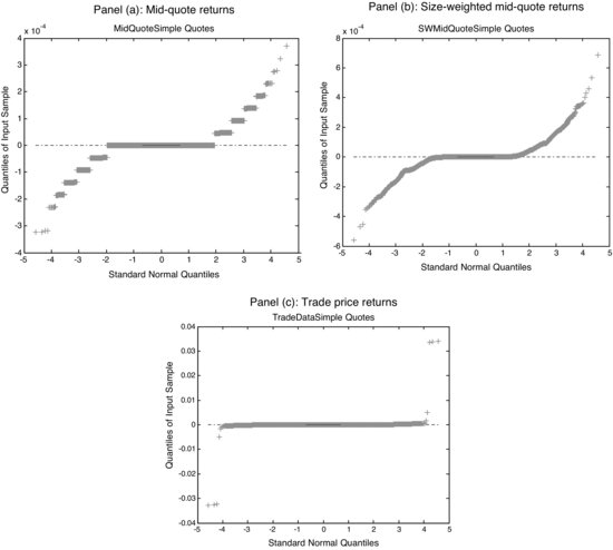
Figure 5 compares the histograms of simple returns computed from mid-quote (panel a), size-weighted mid-quote (panel b), and trade-price (panel c) processes for SPDR S&P 500 ETF data recorded as they arrive throughout November 9, 2009. The data neglect the time difference between the adjacent quotes, treating each sequential quote as an independent observation. Figure 6 contrasts the quantile distribution plots of the same data sets with the quantiles of a standard normal distribution.
As Figures 4 and 5 show, the basic mid-quote distribution is constrained by the minimum “step size”: The minimum changes in the mid-quote can occur at half-tick increments (at present, the minimum tick size is $0.01 in equities). The size-weighted mid-quote forms the most continuous distribution among the three distributions discussed. Figure 6 confirms this notion further and also illustrates the fat tails present in all three types of data distributions.
Figure 4 Bid-Ask Aggregation Techniques on Data for SPDR S&P 500 ETF (ticker SPY) Recorded by NYSE Arca on November 9, 2009, from 14:00:16:400 to 14:00:02:000 GMT

Figure 5 Histograms of Simple Returns Computed from Mid-Quote (panel a), Size-Weighted Mid-Quote (panel b), and Trade-Price (panel c) Processes for SPDR S&P 500 ETF Data Recorded as They Arrive Throughout November 9, 2009
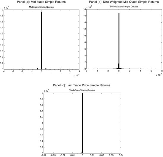
Figure 6 Quantile Plots of Simple Returns of Mid-Quote (panel a), Size-Weighted Mid-Quote (panel b), and Trade-Price (panel c) Processes for SPDR S&P 500 ETF Data Recorded as They Arrive Throughout November 9, 2009
In addition to real-time adjustments to bid-ask data, researchers deploy forecasting techniques to estimate the impending bid-ask spread and adjust for it in models ahead of time. Future realizations of the bid-ask spread can be estimated using the model suggested by Roll (1984), where the price of an asset at time t, pt, is assumed to equal an unobservable fundamental value, mt, offset by a value equal to half of the bid-ask spread, s. The price offset is positive when the next market order is a buy, and negative when the trade is a sell, as shown in equation (3):
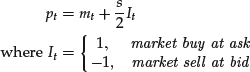
If either a buy or a sell order can arrive next with equal probability, then E[It] = 0, and ![]() , absent changes in the fundamental asset value, mt. The covariance of subsequent price changes, however, is different from 0:
, absent changes in the fundamental asset value, mt. The covariance of subsequent price changes, however, is different from 0:
(4) ![]()
As a result, the future expected spread can be estimated as follows:
![]()
Numerous extensions of Roll’s model have been developed to account for contemporary market conditions along with numerous other variables. Hasbrouck (2007) provides a good summary of the models.
HIGH-FREQUENCY DATA ARE IRREGULARLY SPACED IN TIME
Most modern computational techniques have been developed to work with regularly spaced data, presented in monthly, weekly, daily, hourly, or other consistent intervals. The traditional reliance of researchers on fixed time intervals is due to:
- Relative availability of daily data (newspapers have published daily quotes since the 1920s).
- Relative ease of processing regularly spaced data.
- An outdated view that “whatever drove security prices and returns, it probably did not vary significantly over short time intervals.” (Goodhart and O’Hara, 1997, pp. 80–81)
In contrast, high-frequency observations are separated by varying time intervals. One way to overcome the irregularities in the data is to sample it at certain predetermined periods of time—for example, every hour or minute. For example, if the data are to be converted from tick data to minute “bars,” then under the traditional approach, the bid or ask price for any given minute would be determined as the last quote that arrived during that particular minute. If no quotes arrived during a certain minute, then the previous minute’s closing prices would be taken as the current minute’s closing prices, and so on. Figure 7, panel (a) illustrates this idea. This approach implicitly assumes that in the absence of new quotes, the prices stay constant, which does not have to be the case.
Figure 7 Data-Sampling Methodologies
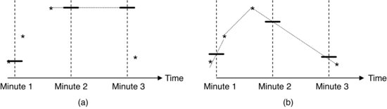
Dacorogna et al. (2001) propose a potentially more precise way to sample quotes—linear time-weighted interpolation between adjacent quotes. At the core of the interpolation technique is an assumption that at any given time, unobserved quotes lie on a straight line that connects two neighboring observed quotes. Figure 7, panel (b) illustrates linear interpolation sampling.
As shown in Figure 7, panels (a) and (b), the two quote-sampling methods produce quite different results.
Mathematically, the two sampling methods can be expressed as follows:
(5) ![]()
Quote sampling using linear interpolation:
(6) ![]()
where ![]() is the resulting sampled quote, t is the desired sampling time (start of a new minute, for example), tlast is the timestamp of the last observed quote prior to the sampling time t, qt,last is the value of the last quote prior to the sampling time t, tnext is the timestamp of the first observed quote after the sampling time t, and qt,next is the value of the first quote after the sampling time t.
is the resulting sampled quote, t is the desired sampling time (start of a new minute, for example), tlast is the timestamp of the last observed quote prior to the sampling time t, qt,last is the value of the last quote prior to the sampling time t, tnext is the timestamp of the first observed quote after the sampling time t, and qt,next is the value of the first quote after the sampling time t.
Figure 8 Mid-Quote “Closing Quotes” Sampled at 200 ms (left) and 15s Intervals
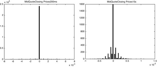
Figure 9 Mid-Quote “Time-Interpolated Quotes” Sampled at 200 ms (left) and 15s Intervals
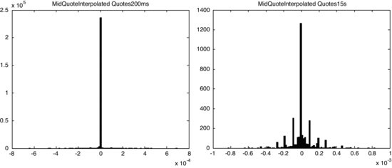
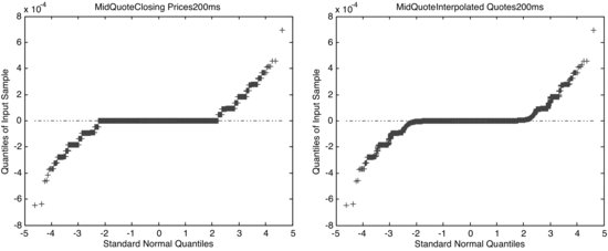
Figures 8 and 9 compare histograms of the mid-quote data sampled as closing prices and interpolated at frequencies of 200 ms and 15s. Figure 10 compares quantile plots of closing prices and interpolated distributions. As Figures 8 and 9 show, often-sampled distributions are sparse, that is, contain more 0 returns than distributions sampled at lower frequencies. At the same time, returns computed from interpolated quotes are more continuous than closing prices, as Figure 10 illustrates.
Figure 10 Quantile Plots: Closing Prices vs. Interpolated Mid-Quotes Sampled at 200 ms
Instead of manipulating the interquote intervals into the convenient regularly spaced formats, several researchers have studied whether the time distance between subsequent quote arrivals itself carries information. For example, most researchers agree that intertrade intervals indeed carry information on securities for which short sales are disallowed; the lower the intertrade duration, the more likely the
yet-to-be-observed good news and the higher the impending price change.
Duration models are used to estimate the factors affecting the time between any two sequential ticks. Such models are known as quote processes and trade processes, respectively. Duration models are also used to measure the time elapsed between price changes of a prespecified size, as well as the time interval between predetermined trade volume increments. The models working with fixed price are known as price processes; the models estimating variation in duration of fixed volume increments are known as volume processes.
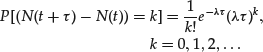
Durations are often modeled using Poisson processes that assume that sequential events, like quote arrivals, occur independently of one another. The number of arrivals between any two time points t and (t + τ) is assumed to have a Poisson distribution. In a Poisson process, λ arrivals occur per unit time. In other words, the arrivals occur at an average rate of (1/λ). The average arrival rate may be assumed to hold constant, or it may vary with time. If the average arrival rate is constant, the probability of observing exactly k arrivals between times t and (t + τ) is
(7) 
Diamond and Verrecchia (1987) and Easley and O’Hara (1992) were the first to suggest that the duration between subsequent ticks carries information. Their models posit that in the presence of short-sale constraints, intertrade duration can indicate the presence of good news; in markets of securities where short selling is disallowed, the shorter the intertrade duration, the higher is the likelihood of unobserved good news. The reverse also holds: In markets with limited short selling and normal liquidity levels, the longer the duration between subsequent trade arrivals, the higher the probability of yet-unobserved bad news. A complete absence of trades, however, indicates a lack of news.
Easley and O’Hara (1992) further point out that trades that are separated by a time interval have a much different information content than trades occurring in close proximity. One of the implications of Easley and O’Hara (1992) is that the entire price sequence conveys information and should be used in its entirety whenever possible, strengthening the argument for high-frequency trading.
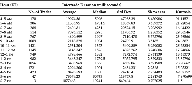
Table 3 shows summary statistics for a duration measure computed on all trades recorded for S&P 500 Depository Receipts ETF (SPY) on May 13, 2009. As Table 3 illustrates, the average intertrade duration was the longest outside of regular market hours, and the shortest during the hour preceding the market close (3–4 P.M. ET).
Table 3 Hourly Distributions of Intertrade Duration Observed on May 13, 2009 for S&P 500 Depository Receipts ETF (SPY)
The variation in duration between subsequent trades may be due to several other causes. While the lack of trading may be due to a lack of new information, trading inactivity may also be due to low levels of liquidity, trading halts on exchanges, and strategic motivations of traders. Foucault, Kadan, and Kandel (2005) consider that patiently providing liquidity using limit orders may itself be a profitable trading strategy, as liquidity providers should be compensated for their waiting. The compensation usually comes in the form of a bid-ask spread and is a function of the waiting time until the order limit is “hit” by liquidity takers; lower intertrade durations induce lower spreads. However, Dufour and Engle (2000) and Saar and Hasbrouck (2002) find that spreads are actually higher when traders observe short durations, contrasting the time-based limit order compensation hypothesis.
In addition to durations between subsequent trades and quotes, researchers have also been modeling durations between fixed changes in security prices and volumes. The time interval between subsequent price changes of a specified magnitude is known as price duration. Price duration has been shown to decrease with increases in volatility. Similarly, the time interval between subsequent volume changes of a prespecified size is known as the volume duration. Volume duration has been shown to decrease with increases in liquidity.
The information content of quote, trade, price, and volume durations introduces biases into the estimation process, however. If the available information determines the time between subsequent trades, time itself ceases to be an independent variable, introducing substantial endogeneity bias into estimation. As a result, traditional estimates of variance of transaction prices are too high in comparison with the true variance of the price series.
KEY POINTS
- High-frequency data are different from daily or lower frequency data. Whereas low frequency data typically comprise regularly spaced open, high, low, close, and volume information for a given financial security recorded during a specific period of time, high-frequency data include bid and ask quotes, sizes, and latest trade characteristics that are recorded sequentially at irregular time intervals.
- The differences affect trading strategy modeling, introducing new opportunities and pitfalls for researchers.
- Numerous data points allow researchers to deduce statistically significant inferences on even short samples of high-frequency data.
- Different sampling approaches have been developed to convert high-frequency data into a more regular format better familiar to researchers, yet diverse sampling methodologies result in datasets with drastically dissimilar statistical properties.
- Some properties of high-frequency data, like intertrade duration, carry important market information unavailable at lower frequencies.
REFERENCES
Aldridge, I. (2009). High-Frequency Trading: A Practical Guide to Algorithmic Strategies and Trading Systems. Hoboken, NJ: John Wiley & Sons.
Corsi, F., Zumbach, G., Müller, U., and Dacorogna, M. (2001). Consistent high-precision volatility from high-frequency data. Economics Notes 30: 183–204.
Dacorogna, M. M., Gencay, R., Muller, U. A., Olsen, R., and Pictet, O. V. (2001). An Introduction to High-Frequency Finance. San Diego, CA: Academic Press.
Diamond, D. W., and Verrecchia, R. E. (1987). Constraints on short-selling and asset price adjustment to private information. Journal of Financial Economics 18: 277–311.
Dufour, A., and Engle, R. F. (2000). Time and the price impact of a trade. Journal of Finance 55: 2467–2498.
Easley, D., and O’Hara, M. (1992). Time and the process of security price adjustment. Journal of Finance 47, 2: 557–605.
Foucault, T., Kadan, O., and Kandel, E. (2005). Limit order book as a market for liquidity. Review of Financial Studies 18: 1171–1217.
Goodhart, C., and O’Hara, M. (1997). High frequency data in financial markets: Issues and applications. Journal of Empirical Finance 4: 73–114.
Hasbrouck, J. (2007). Empirical Market Microstructure: The Institutions, Economics, and Econometrics of Securities Trading. New York: Oxford University Press.
Roll, R. (1984). A simple implicit measure of the effective bid-ask spread in an efficient market. Journal of Finance 39, 4: 1127--1240.
Saar, G., and Hasbrouck, J. (2002). Limit orders and volatility in a hybrid market: The Island ECN. Working paper, New York University.
Voev, V., and Lunde, A. (2007). Integrated covariance estimation using high-frequency data in the presence of noise. Journal of Financial Econometrics 5, 1: 68–104.