Classification and Regression Trees and Their Use in Financial Modeling

MIN ZHU

Business School, Queensland University of Technology, Australia

DAVID PHILPOTTS

QEP Global Equities, Schroder Investment Management, Sydney, Australia

MAXWELL J. STEVENSON, PhD

Discipline of Finance, Business School, University of Sydney, Australia

Classification and regression trees (CART) are nonparametric and nonlinear modeling techniques that essentially use recursive partitioning techniques to separate observations in a binary and sequential fashion. There are two varieties: (1) classification trees when the dependent variable is categorical, and (2) regression trees when the dependent variable is continuous.

Although the approach is not widely utilized within the investment community, the applications of CART to financial markets nevertheless include the classification of financially distressed firms by Frydman, Altman, and Kao (1985), asset allocation by Sorensen, Mezrich, and Miller (1998), equity style timing by Kao and Shumaker (1999), and stock selection by Sorensen, Miller, and Ooi (2000). In this entry we provide an introduction to the CART framework and contrast it to more traditional modeling methods. We then illustrate the technique by applying it to stock selection across the North American equity markets.

TECHNICAL DETAILS

We begin by introducing the standard tree terminology. The root is the top node, which includes all observations in the learning sample. The splitting condition at each node is expressed as an “if-then-else” rule that is determined by a specific splitting criterion. The splitting node is also called the parent and the two descendant subnodes are called children. A node keeps splitting until a terminal node or leaf is reached.

The fundamental idea behind CART is to recursively partition the space until all the subspaces are sufficiently homogenous in order to apply simple models to them. This is in contrast to linear and logistic regressions, the linear parametric counterparts of regression and classification trees, respectively, which are global models where a single predictive formula is imposed over the entire data space. When the dataset has multiple features that interact in complicated and nonlinear ways, as is often the case with financial data, a single global model may inadequately capture the underlying relationships.

There are two major steps in the CART analysis: (1) Build a tree using a recursive splitting of nodes, and (2) prune the tree in order to obtain the optimal tree size so as to prevent overfitting. Each of these two steps will be discussed in more detail below. Breiman et al. (1984) provide a detailed overview of the theory and methodology of CART, including a number of examples from many disciplinary areas. There are also many software packages that implement the CART algorithm. Popular ones include R packages such as rpart and tree and the Matlab function classregtree.

Binary Recursive Partitioning

Let be a learning sample, (xn, yn)}, where xi is a vector of attributes; yi is the response, which can be categorical or continuous; and n is the number of observations. The attribute vector xi belongs to X, the attribute space. The tree-building algorithm involves repeatedly splitting subsets of into two descendant subsets, beginning with itself. For a continuous variable xi, the allowed splits are of the form xi<c versus . For categorical variables the levels are divided into two classes. Therefore, for a categorical variable with K levels, there are 2K−1−1 possible splits, disallowing the empty split and ignoring the order.

Figure 1 A split generates two children of the node t, denoted by tL and tR. A proportion pL of the initial data go into the left child and a proportion of pR go into the right child.

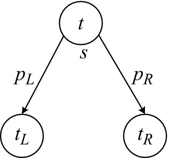
In choosing the best splitting rule, CART seeks to maximize the average purity of the two child nodes. Hence, some criterion measuring data homogeneity or, alternatively, impurity should be introduced. These impurity measures are loosely classed splitting criteria. Let us introduce, for any node t, a measure i(t) that signifies the impurity of the node. Suppose that a candidate split s divides the node into tL and tR such that a proportion pL of the cases in t go into tL and a proportion pR go into tR (see Figure 1). Then the goodness of the split is defined to be the decrease of impurity

For an arbitrary node t and a set of splitting candidates S, the optimal split is chosen to be the one

In other words, the optimal split is the one that reduces impurity by the greatest amount.

The idea for classification and regression trees is quite similar in terms of partitioning methods, which is based on impurity reducing. However, they use different measures of impurity to decode the split.

In a classification problem, suppose that we want to classify data into K classes. At each node t of a classification tree we have a probability distribution ptk, k = 1, …, K, over all K categories. The probabilities are conventionally estimated from the node proportions, such that ptk = ntk/nt, where ntk is the number of observations in the K-th class, and nt is the sample size at node t.

The two most common measures of impurity are the Gini index

and entropy or information

where 0log(0) = 0.

As for regression trees, the most popular impurity measure is

where the constant μt for node t is estimated by the mean of the values of the training data falling into node t.

TREE PRUNING

However, the use of partitioning rules alone cannot guarantee a useful tree model. If reducing impurity is the only goal in tree induction, we will eventually end up with a maximal tree, which has one observation or one class in each leaf, whichever reaches first. This kind of tree adapts too well to the features of the learning sample and has a very high risk of being overfitted. Tree pruning is a way to improve the robustness of the model by trading off in-sample fitting against out-of-sample accuracy. This is particularly important if the model is being used to make predictions.

The best-known procedure for tree pruning is the cost-complexity pruning proposed by Breiman et al. (1984). Let t be a subtree of the maximal tree grown without pruning. Let the size of a tree be the number of terminal nodes. The optimal tree is the one that minimizes the following cost-complexity measure

where α is a complexity parameter to penalize the tree size, and R is the cost, which is commonly taken as misclassification errors in classification cases and deviance in regression cases. For a given value of the complexity parameter α, an optimal tree can be determined. In general, finding the optimal value for α would require an independent set of data (i.e., a testing sample). This requirement is often avoided in practice by using a cross validation procedure.

STRENGTHS AND WEAKNESSES OF CART

Compared to classical parametric models, CART offers a number of benefits in data exploration. In particular, it has a very high degree of interpretability. CART efficiently compresses a large volume of data into an easy-to-understand graphical form that identifies the essential characteristics. It is also very flexible in terms of the structure of the input variables, as either categorical or continuous factors or a combination can be used as inputs. Furthermore, CART is quite robust in the presence of outliers and well suited to noisy datasets, both of which tend to be features of financial data.

Being nonparametric it does not require any assumptions to be made about the underlying distribution of the variables being modeled. The high incidences of extreme events in the financial markets suggest that the supposition of distributional normality is questionable in many areas of finance. While the assumption may in many cases be a fair approximation to the underlying structural relationship, it is quite rare that tests for non-normality or nonlinearity are explicitly assessed in advance even though this information would help to inform the appropriate choice of modeling technique.

The CART approach also departs from traditional modeling methods by determining a hierarchy of input variables that may be closer to the human decision-making processes. Indeed, a key strength of CART over classical modeling methods is that it allows one to represent various types of interactions between variables, particularly conditional relevance. Conditional relevance occurs if a factor is relevant only when it is conditioned upon some other factor. For example, only if a certain condition is met by the first high-level attribute is a second attribute taken into consideration. The same holds for the next attribute in the tree hierarchy, and so on.

Another possible benefit for financial modelers using CART is the diversification of model risk as argued by Philpotts et al. (2011). The widespread use of linear modeling methodologies among quantitative asset managers, taken together with the similarity in data sources and risk models, may in turn have contributed to model risk in financial markets leading to a high degree of commonality in investment decisions. As a less used technique, CART is appealing in the context of potentially offering a degree of model diversification. Philpotts et al. (2011) present empirical evidence highlighting the favorable performance of tree-based models compared to more traditional modeling techniques.

One potential weakness of the recursive partitioning tree construction process is local optimization instead of global optimization. That is, the sequential node-splitting process chooses the next split without attempting to optimize the performance of the whole tree. The resulting tree structure therefore does not guarantee global optimization. Instability is another possible problem in CART solutions. This refers to perturbing a small proportion of the learning sample or resampling the learning sample, which often results in a solution with a very different tree structure. Several alternatives to CART have been developed to address these problems, such as random forests (see Brieman, 2001) and a hybrid approach that combines CART with logistic regression (see Zhu et al., 2011).

APPLICATION OF CART IN STOCK SELECTION

In this section, we provide a detailed example of the CART algorithm as applied to the problem of identifying profitable stocks. This example was specifically chosen so as to provide a contrast with the vast majority of the linear modeling techniques used by financial practitioners. The model was built with monthly stock data from December 1986 to August 2010 covering all liquid stocks listed on the North American equity markets but excluding financial stocks because they would require their own specific model.1 The number of total observations is 279,188 (or 980 stocks per month on average).

At the end of each month, forward total stock returns (price return plus dividends) were calculated. Using the median return of all sample companies in the same period as a proxy of the market return, the excess returns were then computed as the total returns minus the market returns.

A broad spectrum of company valuation and quality-based characteristics, as well as measures of investor sentiment such as price momentum and earnings revisions were selected as reported in Table 1. Instead of using raw values, we use rank orders in order to improve the robustness of the analyses. At each month, the rank order for each variable was computed by first ranking n stocks according to the corresponding variable value, and then dividing the rank by n to scale it between 0 and 1. Furthermore, in order to overcome the high correlation among some of the explanatory variables, nine composite factors were promoted as potential explanatory variables, which were constructed as an equally weighted average of multiple variables as described in Table 1.

Table 1 Input Variables

We built a classification tree with the purpose of predicting subsequent stock performance. Stocks were sorted into two groups, “outperformers” for those with positive excess returns and “underperformers” for the remainder. The induced categorical variable was then used as the dependent variable in the subsequent modeling process. One of the benefits of working with categorical responses instead of raw returns lies in the fact that it alleviates the impact of extreme returns, which may have multiple causes. The tree model was built with the data up to and including April 2007 while the data between May 2007 and August 2010 were reserved for out-of-sample testing. Figure 2 graphically illustrates the hierarchical structure of the stock selection tree.

The first observation to note is that the primary split is valuation based. More specifically, the tree makes a distinction between those stocks that are relatively expensive (the right-hand branch) and those that are not expensive. One of the most attractive nodes splits again on high value and therefore identifies cheap stocks as having a 59.2% probability of outperforming the universe (Node 1). In contrast, the worst performing stocks are characterized by being expensive and exhibiting low profitability (Node 14). Companies with these attributes only have a 42% chance of outperforming.

The tree is able to identify the exception to the rule. For example, while identifying that value was the most important driver of stock returns, the tree also suggests that more expensive stocks still have a good chance of outperforming the market providing that they are blessed with profitability, stability in earnings, strong momentum, and are also associated with strong earnings revisions (Node 10).

Similarly, the decision tree framework also highlights the nonlinear behavior of the stock returns to the underlying predictor variables. For example, stocks in Nodes 3 and 5 have similar outperforming probabilities but are of opposite preference with regard to leverage. Conditional on above-average debt cover, Node 3 actually prefers some degree of leverage and more significantly penalizes overly

Figure 2 Decision Tree for North American stocks built using data from December 1986 to April 2007 to model the chance of a stock outperforming the overall market. The dependent variable is set as an “outperformer” (Out) if a stock subsequently achieves a higher return than the market, and “underperformer” (Und) otherwise. The outperforming probabilities are reported in percentages at each terminal node along with the splitting criteria.

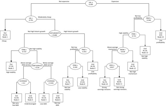
conservative firms (with too low leverage). In contrast, leverage is a characteristic to be avoided among firms that cannot service their debts (Node 5).

Table 2 is an out-of-sample test of the model. Each month from May 2007 until August 2010, we ranked all stocks based upon the predicted outperforming probabilities by the tree model and formed two portfolios. One portfolio is an equal weighting of stocks with the highest half of outperforming probabilities (long), and the second is an equal weighting of the rest expected to underperform (short). Table 2 reports the annualized excess return, the tracking error, the information ratio, and the monthly win rate of the two portfolios. The long portfolio outperformed the benchmark by 2.6% with a similar relative risk. The short portfolio underperformed by 2.8% with a slightly higher tracking error. The monthly win rate is the proportion of months that a portfolio outperformed the benchmark out-of-sample. The tree model achieved a monthly win rate of 57%.

Table 2 Out-of-Sample Performance (May 2007–August 2010). Portfolios were rebalanced monthly and transaction costs were not taken into account.

KEY POINTS

• CART is a flexible modeling technique that offers significant potential to assist in financial decision making.
• CART is a nonparametric modeling technique that does not impose the stringent assumptions required by classical regression analysis, and therefore sidesteps many of the known issues associated with traditional parametric models.
• CART is well suited to identifying nonlinearities and complex interactions in the data. It is minimally affected by missing values, outliers, or multicollinearity.
• Unlike many other methods, CART can be easily visualized, which helps financial decision makers to assess the theoretical support behind the resulting investment insights.
• The hierarchical structure of a tree model may more closely resemble how the human brain makes decisions. In particular, the “if-then-else” nature of the rules in the model emulates an expert system that is able to incorporate the exception to the rule.
• CART also embraces the important feature of conditional relevance, which is widespread in financial data. In the CART framework, input variables are allowed to interact and have different influences under varying conditions.
• As with any other quantitative model development process, care must be taken to ensure the integrity of the input data and that the intended application makes intuitive sense.

NOTE

1. Financial stocks were excluded due to their different accounting structure, which makes comparisons with nonfinancials troublesome, although similarly structured stock selection models can also be applied within the sector.

ACKNOWLEDGMENT

Min Zhu gratefully acknowledges financial support from the Capital Market Cooperative Research Centre (CMCRC).

REFERENCES

Breiman, L. (2001). Random forests. Machine Learning 45: 5–32.

Breiman, L., Friedman, J., Olshen, R., and Stone, C. (1984). Classification and Regression Trees. Belmont, CA: Wadsworth.

Frydman, H., Altman, E. I., and Kao, D. L. (1985). Introducing recursive partitioning for financial classification: The case of financial distress. Journal of Finance 40: 269–291.

Kao, D. L., and Shumaker, D. L. (1999). Equity style timing. Financial Analysts Journal 55: 37–48.

Philpotts, D., Zhu, M., and Stevenson, M. J. (2011). The benefits of tree-based models for stock selection. Working paper.

Sorensen, E. H., Mezrich, J. J., and Miller, K. L. (1998). A new technique for tactical asset allocation. In F. J. Fabozzi, ed., Active Equity Portfolio Management, Chapter 12. New Hope, PA: Frank J. Fabozzi Associates.

Sorensen, E. H., Miller, K. L., and Ooi, C. K. (2000). The decision tree approach to stock selection. Journal of Portfolio Management, Fall: 42–52.

Zhu, M., Philpotts, D., and Stevenson, M. J. (2011). A hybrid approach to combining CART and logistic regression for stock ranking. Journal of Portfolio Management, Fall: 100–109.