
Discounted Cash Flow Methods for Equity Valuation
Sound investing requires that an investor does not pay more for an asset than its worth. There are those who argue that value is in the eyes of the beholder, which is simply not true when it comes to financial assets. Perceptions may be all that matter when the asset is an art object or antique automobile, but investors should not buy financial assets for aesthetic or emotional reasons; financial assets are acquired for the cash flows expected from them in future periods. Consequently, perceptions of value have to be backed up by reality, which implies that the price paid for any financial asset should reflect the cash flows that it is expected to generate.
Realize that at the end of the most careful and detailed valuation, there will be uncertainty about the final numbers, biased as they are by the assumptions that we make about the future of the company and the economy. It is unrealistic to expect or demand absolute certainty in valuation, since cash flows and discount rates are estimated with error. This also means that you have to give yourself a reasonable margin for error in making recommendations on the basis of valuations. Most importantly, realize that the degree of precision in valuations is likely to vary widely across investments. For example, the valuation of a large and mature company, with a long financial history, will usually be much more precise than the valuation of a young company or of a company that is in a sector that is in turmoil.
Implicit often in the act of valuation is the assumption that markets make mistakes and that we can find these mistakes, often using information that tens of thousands of other investors can access. Thus, the argument that those who believe that markets are inefficient should spend their time and resources on valuation whereas those who believe that markets are efficient should take the market price as the best estimate of value, seems to be reasonable. This statement, though, does not reflect the internal contradictions in both positions. Those who believe that markets are efficient may still feel that valuation has something to contribute, especially when they are called upon to value the effect of a change in the way a firm is run or to understand why market prices change over time.
Furthermore, it is not clear how markets would become efficient in the first place, if investors did not attempt to find under- and overvalued stocks and trade on these valuations. In other words, a precondition for market efficiency seems to be the existence of millions of investors who believe that markets are not.
Stock-pricing models are not physical or chemical laws of nature. There is, however, a strong principle of investing that must eventually hold true for all firms over time if they are to have a positive value. This principle is that you should always be able, in your mind, to construct some sort of logical connection between a positive stock price today and a stream of future cash flows to the investor. The logical chain might be long. You might assume that years of start-up losses (earnings are zero or negative) will be followed by more years of all profits being reinvested. But you should be able to envision some connection between today’s positive stock price and a stream of cash flows that will commence someday in the future.
In this entry, we discuss practical methods of valuing a firm’s equity based on discounted cash flow (DCF) models. Although stock and firm valuation is very strongly tilted toward the use of DCF methods, it is impossible to ignore the fact that many analysts use other methods to value equity and entire firms. The DCF model is the subject of this entry. The primary alternative valuation method is relative valuation (RV). Both DCF and RV valuation methods require strong assumptions and expectations about the future. No one single valuation model or method is perfect. All valuation estimates are subject to model error and estimation error. Nevertheless, investors use these models to help form their expectations about a fair market price. Markets then generate an observable market clearing price based on investor expectations, and this market clearing price constantly changes along with investor expectations.
DIVIDEND DISCOUNT MODEL
The dividend discount model (DDM) is the most basic DCF stock approach to equity valuation, originally formulated by Williams (1938). It states that the stock price should equal the present value of all expected future dividends into perpetuity under the assumption that a firm has an infinite life. But you may also have ignored the DDM once you recognized how difficult it is to apply in the real world. The next several paragraphs simply review the basic concepts in order to highlight the complexities that surround implementing the DDM in practice.
Consider an investor who buys a share of stock, planning to hold it for one year. As you know from previous studies, the intrinsic value of the share is the present value, P(0), of the expected dividend to be received at the end of the first year, ED(1), and the expected sales price, EP(1).
Keep in mind that since we live in a world of uncertainty and no human can perfectly forecast the future, future prices and dividends are unknown. Specifically, we are dealing with expected values, not certain values. Under the assumption that dividends can be predictable, given a company’s dividend history, the expected future dividend in the next period, ED(1), can be estimated based on historical trends. You might ask how we can estimate EP(1), the expected year-end price.
According to equation (1), the year-end intrinsic value, P(1), will be
If we assume the stock will be selling for its intrinsic value next year, then P(1) = EP(1), and we can substitute equation (2) into equation (1), which gives
Equation (3) may be interpreted as the present value of dividends plus the expected sales price at the end of a two-year holding period. Of course, now we need to come up with a forecast of EP(2). Continuing in the same way, we can replace the expected price at the end of two years by the intrinsic value at the end of two years. That is, replace EP(2) by [ED(3)+EP(3)]/(1+R), which relates P(0) to the value of dividends over three years plus the expected sales price at the end of a three-year holding period.
More generally, for a holding period of T years, we can write the stock value as the present value of dividends over the T years discounted at an appropriate discount rate, R, that is assumed to remain constant, plus the present value of the ultimate sales price, EP(T):
In short, the intrinsic price of a share of stock is the present value of a stream of payments (dividends in the case of stocks) and a final payment (the sales price of the stock at time T).
The key problems with implementing this model are the uncertainty of future dividends, the lack of a fixed maturity date, and the unknown sales price at the horizon date and the appropriate discount rate. Indeed, one can continue to substitute for a terminal price on out to infinity (INF):
Equation (5) states that the stock price should equal the present value of all expected future dividends in perpetuity. This formula is the DDM in mathematical form. It is tempting, but incorrect, to conclude from the equation that the DDM focuses exclusively on dividends and ignores capital gains as a motive for investing in stock. Indeed, we assume explicitly in equation (4), the finite version of the DDM, that capital gains (as reflected in the expected sales price, EP(T)) are part of the stock’s value. EP(T) is the present value at time T of all dividends expected to be paid after the horizon date. That value is then discounted back to today, time T = 0. The DDM asserts that stock prices are determined ultimately by the cash flows accruing to stockholders, and those are dividends.
Stocks That Currently Pay No Dividend
If investors never expected a dividend to be paid, then this model implies that the stock would have no value. To reconcile the fact that stocks not paying a current dividend do have a positive market value with this model, one must assume that investors expect that someday, at some time T, the firm must pay out some cash, even if only a liquidating dividend.
CONSTANT-GROWTH DDM
The general form of the DDM, as it stands, is still not very useful in valuing a stock because it requires dividend forecasts for every year into the indefinite future. To make the DDM practical, we need to introduce some simplifying assumptions. One useful and common first pass at the problem is to assume that dividends are trending upward at a stable or constant growth rate, g.
For example, if g = 0.05 and the most recently paid dividend was D(0) = 3.81, expected future dividends are
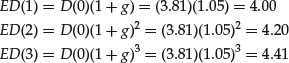
and so on. Using these dividend forecasts, we can solve for intrinsic value as
![]()
Since the basic form of this equation stretches to infinity, basic algebra allows this equation to be written as
Equation (6) is called the constant-growth DDM, or the Gordon-Shapiro model, after Myron Gordon and Eli Shapiro, who popularized the model [see Gordon (1962) and Gordon and Shapiro (1956)].
Equation (6) should remind you of the formula for the present value of perpetuity. If dividends were expected not to grow, g = 0, then the dividend stream would be a simple perpetuity, and the valuation formula would be
![]()
P(0) = ED(1)/(R−g) is a generalization of the perpetuity formula to cover the case of a perpetuity growing at a constant rate, g. As g increases, for a given value of ED(1), the stock price rises. The constant-growth DDM is valid only when g is less than R. If dividends were expected to grow forever (to infinity) at a rate faster than R, the value of the stock would be infinite. Further, in all of the DDM equations presented, R is also assumed to be constant forever.
NONCONSTANT-GROWTH DDM
If you feel that you know the future growth rates in each period for a firm, then you can certainly use unique growth rates, g(T) and required rates of return, R(T), in the present value equation and discount all unique dividends and future selling price back to the present. The problem becomes one of time, effort, and estimation risk. At some future point in time, what you believe to be a better unique estimate of a future dividend or a future discount rate will in reality be no better than an assumption of constant growth and constant discount rate.
INTUITION BEHIND THE DDM
In a market economy, common sense dictates that you should go into business only if you expect to make money. In a sole proprietorship, everything left over from the revenue you earned, minus expenses, is yours. In other forms of a business organization, you need to be a bit more formal because there are other owners. In a partnership, partners draw money out of the business. And shareholders get money out of a corporation by receiving dividends. Using the corporate form as an example, the value per share is determined by the value of the dividends distributed to each shareholder. That is, the value per share is determined by the present value of each shareholder’s expected share of the profits.
Here is a simple example that illustrates several of the uncertainties involved with the basic DCF valuation process for a share of common stock. Let’s say you consider buying shares of a corporation. How much will you pay if the expected annual dividend forever is $10 per share? That depends on how much of an annual “return” you want. If you want a 10% return, you’ll offer $100 (that is, a $10 dividend divided by a $100 investment equals a return of 10%). But just because you offer to pay $100 doesn’t mean someone will sell to you at that price.
Financial capital is subject to principles of market supply and demand, just like commodities. Suppose market conditions are such that prevailing rates of return for corporate shares in this particular risk class are in the 5% range. If I’m selling stock that commands a $10 per share dividend I can demand a price of $200, and someone will give it to me. Suppose this corporation is a bit riskier than most others. A buyer may say, “If I’m willing to accept the prevailing 5% return, there are hundreds upon hundreds of better-quality corporations I can invest in. So if you want me to buy your shares, you need to give me incentive to bypass all the others. The buyer and seller may settle on a 7% return, which is equivalent to a price of about $143. The appropriate required rate of return, R, is therefore critical, and R can vary with market conditions.
In all cases, assuming that the life of the corporation is infinite, the current price, P(0), is computed as the constant dividend in perpetuity, D, divided by the required rate of return, R, that is, the present value of all future constant dividends. Often, though, investors use return, R, as the basis for comparing and pricing investments. R is often estimated from observable information as D (dividend) divided by current price P(0). Mathematically, it looks like this:
![]()
You’ve seen this before. It is the dividend yield.
COMPLICATIONS IN IMPLEMENTING THE DDM IN THE REAL WORLD
As you can see by now, there are essentially four major issues that complicate finding the present value of all future dividends and, therefore, in implementing the DDM.
Expected Growth of Dividends
As profits grow over time (as we hope they will), dividends can be expected to grow and not remain constant forever. If profits and dividends are growing by 10% every year, the dividend this year may be $10, but by next year, it will be $11. If we divide $11 by today’s $200 purchase price, next year’s yield will be 5.5% (11/200). The year after, assuming further 10% growth, the dividend will be $12.10. Dividing that by the $200 purchase price produces a yield of 6.05%. The buyer might smile, but the seller won’t accept it. The seller wants a price that truly is consistent with the prevailing 5% yield. At $200, the buyer gets too much of a good deal. If the latter holds the stock over time, he’ll wind up with an annual return well in excess of 5%.
Appropriate Expected Required Rate of Return
Simply stated, present value is a tool for computing today’s equivalent of a cash payment to be made tomorrow. As stated earlier, this is often referred to as DCF valuation. If I offer you $10 today or $10 a year from now, you’ll probably choose $10 today. But if the choice is $10 today or $11.50 a year from now, you have to pause. If you can invest today’s $10 payment for one year at 5%, at the end of the year you’ll have $10.50. But if you bypass the $10 for now and wait, you can get $11.50 a year hence. That’s a better deal. The way to decide if you should wait is to do some mathematics that helps you decide how much you must receive today to allow you to invest and wind up with $11.50 a year hence. In this example, the “present value” of $11.50 one year from now, assuming a 5% return, is $10.95. If I take $10.95 and invest it for one year at 5%, I’ll wind up with $11.50 at the end of the year. If interest rates rise, to say 8%, it’ll take less money today to generate $11.50 a year hence ($10.65 will be sufficient). So as interest rates rise, present values fall, and vice versa.
Expected Future Selling Price
Thus far, we have thought about a stream of dividends stretching into the infinite future. Even long-term investors prefer a holding period that’s something short of infinity. So we need to account for the fact that someday you’ll want to sell your shares. As such, the proceeds you expect to get when you sell are included, along with dividends, in the stream of cash you expect to get, and that goes into the present value calculation.
Let’s think about a projection of the future sale price. If you think you may sell in two years, imagine how a prospective buyer, two years into the future, will value the dividend stream that he’ll get. Continuing with the preceding example, he’ll be looking at an initial payout of $12.10 and a 5% return. So a price of $244 seems a reasonable starting point. Of course, you’ll need to make adjustments for probable growth beyond year two. And perhaps 5% won’t be appropriate as a rate of return. Market rates may rise or fall, and/or the quality of the corporation may improve or deteriorate relative to alternative investments. And two years hence, the growth forecast may change. But in any case, we do have a $244 starting point. The changes may bring it up, perhaps to $275, or down, possibly to $175. But if an exuberant analyst publishes a target price of $1,000, you ought to raise an eyebrow and insist that the analyst get serious about justifying his presumably bold assumptions about market rates, growth, or company quality.
Reinvestment of Profits/Internal Financing that Support Growth
It is standard for corporations to refrain from paying out all annual profit as dividend. Some money is held in the business for a rainy day. And some money is simply reinvested for future growth. Either way, profits not paid out as dividends are known as retained earnings. Reinvestment is more desirable than dividend payments if the corporation can earn a higher return on the money than the shareholder could get (by reinvesting the dividends). If all goes well, the reinvestment will enable the corporation to pay a higher dividend in the future than would otherwise have been the case. Going back to the preceding example, if reinvestment gives the corporation the ability to set a year-five payout at $18 rather than $12.10, that raises the starting-point target price to $360. A shareholder who accepts a forecast like that would likely forgo all or some immediate dividend payments in order to get that bigger future reward. As you can see, even if a corporation currently pays little or no dividend, we still have to acknowledge dividends as a major factor in our thoughts about share pricing.
For better or worse, many corporations now see themselves as “growth” companies. And many shareholders have accepted a situation where these publicly traded growth companies pay out very little of their profits, if anything, as dividends, and reinvest most or all profits back into the business. Many companies do not deliver nearly as well on the growth dream as everybody hopes. But the growth culture remains alive and well, and the dividend payout ratio has declined.
ADAPTING TO THE COMPLICATIONS: THE EARNINGS PER SHARE APPROACH
As a result of the four complications listed, modern stock prices have become uncoupled from dividends. So, in the real world, it is difficult to compute a fair price through the basic dividend formulas presented.
Here is one solution. It involves substituting earnings per share (EPS) for dividends. This doesn’t really work in a theoretical DDM sense, but it does work within the context of a growth culture. Shareholders have so thoroughly accepted and adopted growth that they act as if all corporate EPS (whether paid as dividends or reinvested back into the business) is in their hands. So, instead of working with a dividend yield as presented earlier, we can substitute an earnings (E) yield, which is computed as follows:
![]()
Does the E/P ratio look familiar? It should. Turn it upside down and we get something you see all the time: the P/E (price/earnings) ratio.
It is important to emphasize that P/E ratios are not just one of those things we use for the heck of it. They have a serious and solid intellectual underpinning. They are equivalent to earnings yields, which are the modern-day substitute for dividend yields—the true basis for valuing ownership of corporate stock. So when somebody states that P/E ratios are no longer relevant, you’d best turn away. Buying any stock without addressing the P/E ratio is not sensible.
When we flip P/E back over and think of earnings yield, we can understand, from the prior discussion of dividend yield, that a bad company’s stock will have to offer a higher yield to attract buyers. Similarly, the yield for a great company will be low (otherwise, there would be too many would-be buyers). Let’s see how this works when we flip the earnings yields back to P/Es.
If EPS equals $3.00 and the earnings yield is 5%, the price will be $60. If it’s a bad company and the yield is higher, at 8%, the stock price will be $37.50. If it’s a good company and the yield is lower, say 3%, the stock price will be $100. The starting number translates to a P/E as follows: a $60 price divided by $3.00 EPS gives us a P/E of 20. A bad-company stock price of $37.50 divided by EPS of $3.00 produces a P/E of 12.5. A good-company stock price of $100 divided by EPS of $3.00 produces a P/E of 33.3.
That’s the basis for the generally recognized phenomenon of good stocks having higher P/Es and bad stocks generally having lower P/Es. So, once again, this isn’t just one of those things. It’s an inevitable result of the basic principles of finance and math. When evaluating companies, good or bad is usually determined based on growth prospects and risk.
We handled the complicating factors by treating EPS as if it were the same as a dividend. But notwithstanding, we still have a reasonably rational basis for stock prices. We can argue over what the growth prospects are and what the market return ought to be (based on differing assessments of market conditions and company-quality issues). So there will always be disagreement on what, exactly, a fair stock price ought to be. But all rational investors should be somewhere in the same ballpark. We may have a big ballpark and debate if a stock that commands $25 today is worth $15 or $35. But we are unlikely to seriously consider a price of, say, $350.
FREE CASH FLOW DCF MODEL—TOTAL FIRM VALUATION
While estimating future cash flows to an individual share of stock can seem daunting, some investors prefer to estimate the free cash flow to the entire firm. Doing this allows investors to estimate the value of the entire firm and then “back out” an estimated value of a share of stock. This is called the free cash flow (FCF) model. While legitimate accounting rules do enable managers and auditors some range of choices, at the end of the day, good companies wind up looking good and bad companies wind up looking bad. In short, there’s no one number in an income report that truly gives you the necessary information to value a firm from a discounted expected future cash flow viewpoint. You still have to select which type of cash flow you’re going to look at. But the choice becomes very easy once you ask yourself the following question: What’s my specific purpose for wanting to know how a company is doing?
There are many different types of users of financial information, and each is best served by concentrating on the information most relevant to him/her. Let’s look at various kinds of numbers and consider what they say, and what types of investors will find them most useful.
Generally accepted accounting principles (GAAP) is a set of formal rules that produces what most of us have come to accept as the most official, or standard, version of income that a public corporation can report. Novices often believe this is the only valid number and are perplexed to learn otherwise. Essentially, GAAP is simple: Revenues minus costs equal profits. But the world is a complex place. For our convenience, we divide our activities into time periods. In a simple world, all costs would be incurred in the same period as the revenues with which they are associated. But that is often not the case, so accountants have to find ways to identify which expenses should be matched against which revenues. One example is depreciation, a concept used to allocate multiperiod costs of a given expense to all the periods in which the expense generates revenue (e.g., if a factory can produce revenue for 10 years, charge one-tenth of the cost to build it against revenue in each year).
Observers correctly note that depreciation rules are artificial, and advocate use of other performance measures that are supposedly more “real.” We’ll touch on this later. But for now, it’s important to understand that depreciation rules are motivated by good purpose. They, and other GAAP rules, are designed to paint a picture of the “economic” performance of the business, something that is not necessarily the same as a running tally of physical dollars coming in and going out within a specific period of time.
If you are looking to see how a company is doing because you want to form an opinion as to whether or not it has a track record of “success” (defined however you wish), GAAP income is very important to you.
As noted, many investors do not like GAAP because of the artificial nature of depreciation. Their objection is valid. GAAP is, indeed, imperfect. Companies have latitude to determine how to calculate it. They don’t always use an equal allocation for each year. It’s difficult, if not impossible, to reliably estimate useful life, especially since assets are usually enhanced (that is, factories modernized) as time passes, thereby giving rise to extended life and additional depreciable expenses tacked on. An assumption that at the end of the depreciation period the asset will be worth zero, or some predetermined salvage value, is often untrue in the real world. And besides, there are other kinds of “artificial” revenue-expense matching formulations to cover other situations. But depreciation is usually the biggest objection.
Difference between Cash Flow and Free Cash Flow
The response is often to add depreciation back to net income to calculate cash flow. This can be a trap for the unwary. The phrase “cash flow” sounds comforting. After all, how much more reliable a gauge of performance can you seek than cash in minus cash out? Read the warning label closely. Is the cash flow you’re seeing truly computed by adding depreciation back to net income? If that’s what’s happening, be very careful. Companies spend money to enhance their assets every year. Because it is understood that the benefits of these expenditures will span many years, they are not put on the income statement in any single year. So, in truth, simple cash flow understates a company’s true cash-in minus cash-out situation. The solution lies in the firm’s free cash flow. To arrive at a firm’s FCF, we start with net income, add back the noncash depreciation charge, and then subtract the year’s capital-spending outlays. (There are other adjustments, such as those relating to dividends and changes in net working capital; but for now, these simple adjustments will suffice.)
Once you hone in on FCF, you aren’t likely to be misled regarding liquidity. But that does not mean you are learning about general corporate success or failure. Capital-spending programs aren’t “smooth.” In some years, expenditures are very large as major programs ramp up. In other years, capital spending shrinks as these programs wind down toward completion. If we’re in a heavy-spending year, FCF could be negative, even though the company may be having a great year.
DCF valuation depends on the construction of pro forma financial statements in order to estimate a firm’s future cash flows. Pro forma is Latin for “as if.” This measure shows how a company might perform in the future “as if” it performs as it has in the past and other assumptions that are made by the analyst. In any event, it is necessary to construct pro forma financial statements in order to estimate future free cash flows that are the basis for total firm valuation.
CALCULATING FCF
Operating cash flow (OCF) is defined as being equal to earnings before interest and taxes (EBIT) minus taxes plus depreciation. Note, though, that cash flows cannot be maintained over time unless depreciating fixed assets are replaced. That is, the firm must reinvest in those assets that are depreciating (wearing out) so that it can stay alive. Interest paid or any other financing costs such as dividends or principal repaid are not subtracted because we are interested in the cash flow generated by the assets of the firm. The particular mixture of debt and equity a firm actually chooses to use is a managerial decision and determines how the OCF is distributed between owners (equity holders) and creditors (debt holders). The mixture also determines the firm’s weighted average cost of capital (WACC), which impacts the firm’s value through the discount rate.
![]()
Net operating profit after tax (NOPAT) is defined as EBIT minus taxes.
![]()
As a result, OCF can also be written as NOPAT plus any noncash adjustments. Where depreciation is the only noncash adjustment:
![]()
Free cash flow is defined as being the cash flow actually available for distribution to investors after the company has made all the investments in fixed assets and working capital necessary to sustain ongoing operations. To be more specific, the value of a company’s operations depends on all the future expected FCFs, defined as OCF minus the amount of investment in working capital and fixed assets necessary to sustain the business. Thus, FCF represents the cash that is actually available for distribution to investors. Therefore, the way for managers to make their companies more valuable is to create a sustainable increase in the firm’s FCF.
![]()
Let’s illustrate this. Assume a firm has NOPAT of $170.3 million. Its OCF is NOPAT plus any noncash adjustments as shown on the statement of cash flows. Where depreciation is the only noncash charge, the operating cash flow is:
![]()
Further, assume the firm had $1,455 million of operating assets, or operating capital, at the end of the year, but $1,800 million at the end of the next year. Therefore, during the year:
![]()
However, the firm took $100 million of depreciation. We find the gross investment in operating capital as follows:

FCF in the year is:
![]()
Even though the firm had a positive OCF, its very high investment in operating capital resulted in a negative FCF. Since FCF is what is available for distribution to investors, not only was there nothing for investors, but investors actually had to provide more money to the firm to keep the business going.
Table 1 Free Cash Flow Statement: Indirect Method
| Net Income (Net Earnings) | |
| + Depreciation | Depreciation is a noncash expense, and therefore is added back to calculate cash flows. |
| − Increase in accounts receivable (A/R) | The increase in A/R represents sales that have not yet been collected, and therefore did not produce a cash inflow. |
| − Increase in inventories | The increase in inventory has not been recognized as part of cost of goods sold (COGS) but was fully paid for, and therefore is deducted from the cash flow. |
| + Increase in accounts payable (A/P) | The increase in A/P represents costs that have not yet been paid, and therefore is added back to the cash flow. |
| + Increase in taxes payable | Like the increase in A/P, these taxes have not yet been paid. |
| + After-tax interest expense | We want to evaluate the operating side of the business and its financial side separately. The interest payment is a financial expense, and therefore we add back the “net interest cost.” |
| = Operating cash flow (OCF) | |
| − Gross investment in property, plant, and equipment (PP&E), at cost | Some of the cash from operations must be used to buy the assets, such as equipment and plants that will allow the firm to generate future income. This is cash that cannot be freely used to pay dividends, to buy back shares, to repay loans, and the like, and therefore is deducted from the OCF to arrive at the FCF. |
| = Free cash flow (FCF) | This is the cash that the firm can use to distribute to any and all of its suppliers of capital, such as stockholders, debt holders, and warrant holders. |
Table 2 Free Cash-Flow Statement: Direct Method
| Sales | As recorded on the Income Statement |
| − COGS+SG&A | Cost of goods sold (COGS) + Selling, general and administrative expenses (SG&A) |
| − Increase in accounts receivable (A/R) | Credit sales are recorded as income but do not generate a cash inflow. Thus, to adjust “sales” to cash basis, we deduct the increase in A/R. |
| − Increase in inventory | Inventory was paid for and thus represents a cash drain. |
| + Increase in accounts payable (A/P) | A/P are expenses not yet paid. |
| + Depreciation | Depreciation is not a cash expense and is netted out. |
| − Tax on operating income | The difference between taxes on operating income and the increase in taxes payable is the tax shield on interest, which we don’t want to include in the OCF |
| + Increase in taxes payable | |
| = Operating cash flow (OCF) | |
| − Gross investment in property, plant & equipment (PP&E) at cost | |
| = Free cash flow (FCF) |
Is a negative FCF always bad? It depends on why the FCF was negative. If FCF was negative because NOPAT was negative, this is a bad sign, because the company probably is experiencing operating problems. Exceptions to this might be start-up companies, or companies that are incurring significant current expenses to launch a new product line. Also, many high-growth companies have positive NOPAT but negative FCF due to new investment in operating assets needed to support growth. There is nothing wrong with profitable growth, but at some point in time FCF must turn positive in order for a firm to have value. We will see this later in a firm valuation example.
USING THE CASH-FLOW STATEMENT TO ARRIVE AT OCF AND FCF
As stated earlier, FCF is a concept that defines the amount of cash that the firm can distribute to security holders. There are two principal techniques to calculate the FCF—the indirect method and the direct method. Tables 1 and 2 illustrate the direct and the indirect methods of converting accounting earnings into FCFs. The indirect approach first converts the net income (NI) to OCF then to FCF. The direct approach converts each item in the income statement to cash basis.
The indirect method of calculating cash flows starts with the firm’s NI and makes appropriate adjustments to arrive at a number that shows how much cash the firm has taken in over the period. The adjustments that have to be made to NI are of two types—operational adjustments and financial adjustments. When a firm pays interest, net income is defined as
![]()
The following adjustments must be made in order to present the results of the business activity of the firm on a cash basis as explained later in this entry.
Adjustments for Changes in Net Working Capital
Adjustments for changes in net working capital (ANWC) are made because not all the sales are made in cash and because not all the firm’s expenses are paid out in cash. The term and notation are somewhat misleading: Not all the firm’s working capital items are operationally related; since we are interested in cash derived from the ongoing business activity of the firm, we ignore all other current items in our ANWC. Cash and marketable securities are the best example of working capital items that we exclude from our definition of ANWC, as they are the firm’s stock of excess liquidity. Another working capital item that we exclude from the adjustment is notes payable or short-term borrowing. Since our aim in the FCF statement is to calculate the cash available to the firm from its business activities, we exclude from the FCF statement any cash flows relating to the firm’s financing activities—short term or long term.
Adjustments for Investment in New Fixed Assets
When investment in these assets is necessary for the ongoing business activity of the firm, it cannot be used to pay security holders and thus must be deducted to calculate the FCF.
Adjustments for Depreciation and Other Noncash Expenses
Although depreciation is an expense for tax and financial reporting purposes (thus lowering earnings before taxes [EBT] and hence profits after taxes—[NI]), it is by itself not a cash expense. In the FCF statement, we thus add the depreciation back to NI. The remaining effect of depreciation and other noncash expenses on the FCF is the tax savings they entail.
Financial Adjustments
Financial adjustments are adjustments for financial items included in NI. Since FCF is a concept that relates to the ongoing business (as opposed to financial) activities of the firm, we want to neutralize financial items when converting NI into FCF. Thus, for example, although NI includes interest as an expense, we will add back the after-tax interest expenses to obtain the FCF.
The concept of FCF is of cash flows that are generated by the business activities of the firm and are available (that is, “free”) for distribution to all suppliers of capital, such as equity holders, bondholders, convertible holders, and preferred stockholders. The calculation of accounting earnings (net income), however, is done from the point of view of shareholders, which is only one group of capital suppliers.
After calculating the FCFs, we consider their uses. The FCFs can be paid to any security holder of the firm, such as debt holders, stockholders, warrant holders, and convertible bondholders.
Table 3 Cash Flow Statement
| Periodic payments | Interest
Preferred dividend Regular dividend And so on |
These periodic payments to the capital suppliers of the firm are after tax! (The free cash flows [FCFs] from which we pay these financial flows are also after-tax cash flows!) |
| Capital market transactions | Retirement of securities
Debt retirement Preferred stock retirement Share repurchase And so on New financing New bank loans New bond flotation Stock sale Exercise of warrants And so on |
These sums represent cash paid when old securities are retired or represent cash received when new securities are affiliated (privately or publicly). |
| Change in cash | =FCF − financial cash flows |
The cash flows paid to the security holders are the financial cash flows, which include interest, dividends, principal repayment, share repurchases, and funds received upon the issuance of new securities. Obviously, when the FCF is negative (e.g., because growth opportunities necessitate large investments in fixed assets), the financial cash flows must be a net inflow of funds net new financing (of, say, the needed investments).
The difference between the funds generated by the firm’s business, the FCF, and the funds distributed to the security holders of the firm, the financial cash flows (see Table 3), is the change in cash over the period.
Thus, the bottom line of the cash flow statement is the closing link of the three accounting statements of financial performance:
- The income statement’s bottom line-retained earnings feeds into the closing balance sheet as the increase in accumulated retained earnings.
- The income statement and the beginning and closing balance sheets are the basis for the computation of the cash flow statements.
- The last line of the cash flow statement—change in cash (and cash equivalents)—feeds back into the end-of-period balance sheet’s cash account.
The cross-reference of the three accounting statements means that we can use accounting methods to ensure that models of projected financial performance are internally consistent. The firm’s income statement and its cash flow statement are often the basis for predictions of its future FCFs. Note, however, that these statements reflect the past performance of the firm and are not, in themselves, necessarily predictive of future firm performance.
VALUING THE TOTAL FIRM
Earlier we introduced several equations for valuing a firm’s common stock. For example, review the constant growth dividend discount model and the nonconstant growth dividend discount model. These models (equations) have one common element: They all assume that the firm is currently paying a dividend. However, consider the situation of a start-up company formed to develop and market a new product. Such a company generally expects to have low sales during its first few years as it develops and begins to market its product. Then, if the product catches on, sales will grow rapidly for several years. Growing sales require additional assets. A company cannot grow without increasing its assets. Moreover, increasing a liability and/or equity account must finance asset growth.
Small firms can often obtain some bank credit, but they must maintain a reasonable balance between debt and equity. Thus, additional bank borrowings require increases in equity, but small firms have limited access to the stock market. Moreover, even if they can sell stock, their owners are often reluctant to do so for fear of losing voting control. Therefore, the best source of equity for most small businesses is from retaining earnings, so most small firms pay no dividends during their rapid-growth years. Eventually, most successful firms do pay dividends, with dividends growing rapidly at first but then slowing down as the firm approaches maturity.
Although most larger firms do pay a dividend, some firms, even highly profitable ones, have never paid a dividend. How can the value of such a company be determined? Similarly, suppose you start a business and someone offers to buy it from you. How could you determine its value, or that of any privately held business? Alternatively, suppose you work for a company with a number of divisions. How could you determine the value of one particular division that the company wants to sell? In none of these cases could you use the dividend growth model. However, you could use the FCF model to estimate total firm value, then back out the value of equity.
Table 4 XYZ Inc.: Income Statements (in millions except for per-share data)
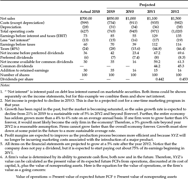
Table 5 XYZ Inc.: Balance Sheets (millions of dollars)

ESTIMATING TOTAL FIRM VALUE USING THE FCF MODEL
Tables 4 and 5 contain the actual 20X8 and projected 20X9 to 20Y2 financial statements for XYZ Inc. The negative FCF in the early years is typical for young, high-growth companies. Even though NOPAT is positive in all years, FCF is negative because of the need to invest in operating assets. The negative FCF means the company will have to obtain new funds from investors, and the balance sheets in Table 5 show that notes payable, long-term bonds, and preferred stock all increase from 20X8 to 20X9.
Assume that XYZ’s cost of capital is 10.84%. To find its going-concern value, we use an approach similar to the nonconstant dividend growth model, proceeding as follows:
Stockholders will also help fund XYZ’s growth. They will receive no dividends until 20Y1, so all of the net income from 20X8 to 20Y1 will be reinvested. However, as growth slows, FCF will become positive, and XYZ plans to use some of its FCF to pay dividends beginning in 20Y1. A variant of the constant growth dividend model can be used to find the value of XYZ’s operations once its FCF stabilize and begin to grow at a constant rate:
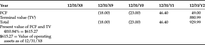
Based on a 10.84% cost of capital, a $49 million FCF in 20Y2, and a 5% growth rate, the value of XYZ’s operations as of December 31, 20Y2 (terminal value) is forecasted to be $880.99 million:
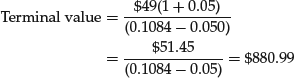
This $880.99 million figure is called the company’s terminal or horizon value, because it is the value at the end of the forecast period. Moreover, this is the amount that XYZ could expect to receive if it sold its operating assets on December 31, 20Y2.
Table 6 shows the free cash flow for each year during the nonconstant growth period, along with the value of operations in 20Y2, at the end of the nonconstant growth period. To find the value of operations as of “today,” December 31, 20X8, we find the PV of each annual cash flow in Table 7, discounting at the 10.84% cost of capital.
The sum of the PVs (all FCFs and the terminal value discounted at 10.84%) is approximately $615 million. The $615.27 represents an estimate of the price XYZ could expect to receive if it sold its operating assets today, December 31, 20X8. The total value of any company is the value of its operations plus the value of its nonoperating assets. As the December 31, 20X8, balance sheet in Table 5 shows, XYZ had $63 million of marketable securities on that date. Unlike operating assets, we do not have to calculate a present value for marketable securities because short-term financial assets as reported on the balance sheet are at, or close to, their market value.
Therefore, XYZ’s total value on December 31, 20X8, is $615.27 + $63.00 = $678.27 million. If the company’s total value on December 31, 20X8, is $678.27 million, what is the value of its common equity?
First, Table 5 shows that notes payable and long-term debt total $123 + $124 = $247 million, and these securities have the first claim on assets and income. (Accounts payable and accruals were netted out earlier.) Next, the preferred stock has a claim of $62 million, and it ranks above the common.
Therefore, the value left for common stockholders is $678.27 − $247 − $62 = $369.27 million.
Table 8 summarizes the calculations used to find XYZ’s stock value per share. There are 100 million shares outstanding, and their total value is $369.27 million. Therefore, the value of a single share is $3.69 ($369.27/100 = $3.69).
Much can be learned from the total firm valuation model, so many analysts today use it for all types of valuations. The process of projecting the future financial statements can reveal quite a bit about the company’s operations and
Table 6 Calculating XYZ’s Pro Forma Expected Free Cash Flow (in millions)
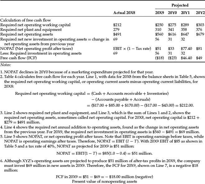
Table 7 Process for Finding the Value of Operations Assumes g = 5% (constant) for Years 12/31/Y2 in Perpetuity
financing needs. Also, such an analysis can provide insights into actions that might be taken to increase the company’s value.
Table 8 Finding the Value of XYZ’s Stock (in millions except for per-share data)
| 1. Value of operations (net of payables and accruals) | $615.27 |
| 2. Plus value of nonoperating assets | $63.00 |
| 3. Total market value of the firm | $678.27 |
| 4. Less: Value of debt | $247.00 |
| Value of preferred stock | $62.00 |
| 5. Value of common equity | $369.27 |
| 6. Divide by number of shares | 100 |
| 7. Estimated value per share | $3.69 |
KEY POINTS
- The two most commonly used approaches for equity valuation are the discounted cash flow and relative valuation models.
- Despite the fact that equity valuation is very strongly tilted toward the use of discounted cash flow models, it is impossible to ignore the fact that many financial modelers employ relative valuation techniques.
- Expected future cash flow is the true basis for financial value. Take the firms that look attractive based on “fundamentals” and attempt to estimate their current fair value based on the present value of all expected future cash flows (dividends and future selling price).
- The basic source of estimation risk when using discounted cash flow models in calculating the value of any financial asset is that the present value depends on expected future cash flows and the appropriate discount rates that reflect the risk of the future cash flows. Cash flow valuation models, therefore, rely on assumptions (often extreme).
- With cash flow valuation, the main problem is estimation risk. No financial modeler can correctly and consistently forecast the future. Estimation risk comes from not being able to perfectly forecast future cash flows and discount rates.
REFERENCES
Gordon, M. J. (1956). Capital equipment analysts: The required rate of profit. Management Science 3, 1: 102–110.
Gordon, M. J. (1962). The Investment, Financing, and Valuation of the Corporation. Homewood, IL: Richard D. Irwin.
Williams, J. B. (1938). The Theory of Investment Value. Cambridge: Harvard University Press.