
Forecasting Stock Returns
In contrast to forecasting events such as the weather, forecasting stock prices and returns is difficult because the predictions themselves will produce market movements that in turn provoke immediate changes in prices, thereby invalidating the predictions themselves. This leads to the concept of market efficiency: An efficient market is a market where all new information about the future behavior of prices is immediately impounded in the prices themselves and therefore exploits all information.
Actually the debate about the predictability of stock prices and returns has a long history.1 More than 75 years ago, Cowles (1933) asked the question: “Can stock market forecasters forecast?” Armed with the state-of-the-art econometric tools at the time, Cowles analyzed the recommendations of stock market forecasters and concluded, “It is doubtful.” Subsequent academic studies support Cowles’s conclusion. However, the history goes further back. In 1900, a French mathematician, Louis Bachelier, in his doctoral dissertation in mathematical statistics titled Théorie de la Spéculation (The Theory of Speculation), showed using mathematical techniques why the stock market behaves as it does.2 He also provided empirical evidence based on the French capital markets at the turn of the century. He wrote:
Past, present, and even discounted future events are reflected in market price, but often show no apparent relation to price changes. . . . [A]rtificial causes also intervene: the Exchange reacts on itself, and the current fluctuation is a function, not only of the previous fluctuations, but also of the current state. The determination of these fluctuations depends on an infinite number of factors; it is, therefore, impossible to aspire to mathematical predictions of it. … [T]he dynamics of the Exchange will never be an exact science. (Bachelier, 1900)
In other words, according to Bachelier, stock price movements are difficult to forecast and even explain after the fact.
Despite this conclusion, the adoption of modeling techniques by asset management firms has greatly increased since the turn of the century. Models to predict expected returns are routinely used at asset management firms. In most cases, it is a question of relatively simple models based on factors or predictor variables. However, more statistical or econometric-oriented models are also being experimented with and adopted by some asset management firms, as well as what are referred to as nonlinear models based on specialized areas of statistics such as neural networks and genetic algorithms.
Historical data are often used for forecasting future returns as well as estimating risk. For example, a portfolio manager might proceed in the following way: Observing weekly or monthly returns, the portfolio manager might use the past five years of historical data to estimate the expected return and the covariances by the sample mean and sample covariances. The portfolio manager would then use these as inputs for mean-variance optimization, along with any ad hoc adjustments to reflect any views about expected returns on future performance. Unfortunately this historical approach most often leads to counterintuitive, unstable, or merely “wrong” portfolios generated by the mean-variance optimization model. Better forecasts are necessary. Statistical estimates can be very noisy and typically depend on the quality of the data and the particular statistical techniques used to estimate the inputs. In general, it is desirable that an estimator of expected return and risk have the following properties:
- It provides a forward-looking forecast with some predictive power, not just a backward-looking historical summary of past performance.
- The estimate can be produced at a reasonable computational cost.
- The technique used does not amplify errors already present in the inputs used in the process of estimation.
- The forecast should be intuitive, that is, the portfolio manager should be able to explain and justify them in a comprehensible manner.
In this entry, we look at the issue of whether forecasting stock returns can be done so as to generate trading profits and excess returns. Because the issue about predictability of stock returns or prices requires an understanding of statistical concepts, we will provide a brief description of the relevant concepts in probability theory and statistics. We then discuss the different types of predictive return models that are used by portfolio managers.
THE CONCEPT OF PREDICTABILITY
To predict (or forecast) involves forming an expectation of a future event or future events. Since ancient times it has been understood that the notion of predicting the future is subject to potential inconsistencies. Consider what might happen if one receives a highly reliable prediction that tomorrow one will have a car accident driving to work. This might alter one’s behavior such that a decision is made not to go to work. Hence, one’s behavior will be influenced by the prediction, thus potentially invalidating the prediction. It is because of inconsistencies of this type that two economists in the mid 1960s, Paul Samuelson and Eugene Fama, arrived at the apparently paradoxical conclusion that “properly anticipated prices fluctuate randomly.”3
The concept of forecastability rests on how one can forecast the future given the current state of knowledge. In probability theory, the state of knowledge on a given date is referred to as the information set known at that date. Forecasting is the relationship between the information set today and future events. By altering the information set, the forecast changes. However, the relationship between the information set and the future is fixed and immutable. Academicians and market practitioners adopt in finance theories this concept of forecastability. Prices or returns are said to be forecastable if the knowledge of the past influences our forecast of the future. For example, if the future returns of a firm’s stock depend on the value of key financial ratios, then those returns are predictable. If the future returns of that stock do not depend on any variable known today, then returns are unpredictable.
As explained in the introduction to this entry, the merits of stock return forecasting is an ongoing debate. There are two beliefs that seem to be held in the investment community. First, predictable processes allow investors to earn excess returns. Second, unpredictable processes do not allow investors to earn excess returns. Neither belief is necessarily true. Understanding why will shed some light on the crucial issues in the debate regarding return modeling. The reasons can be summed up as follows. First, predictable processes do not necessarily produce excess returns if they are associated with unfavorable risk. Second, unpredictable expectations can be profitable if the expected value is favorable.
Because most of our knowledge is uncertain, our forecasts are also uncertain. Probability theory provides the conceptual tools to represent and measure the level of uncertainty.4 Probability theory assigns a number—referred to as the “probability”—to every possible event. This number, the probability, might be interpreted in one of two ways. The first is that a probability is the “intensity of belief” that an event will occur, where a probability of 1 means certainty.5 The second interpretation is the one normally used in statistics: Probability is the percentage of times (i.e., frequency) that a particular event is observed in a large number of observations (or trials).6 This interpretation of probability is the frequentist interpretation, also referred to as the relative frequency concept of probability. Although it is this interpretation that is used in finance and the one adopted in this book, there are attempts to apply the subjective interpretation to financial decision making using an approach called the Bayesian approach.7
With this background, let’s consider again the returns of some stock. Suppose that returns are unpredictable in the sense that future returns do not depend on the current information set. This does not mean that future returns are completely uncertain in the same sense in which the outcome of throwing a die is uncertain. Clearly, we cannot believe that every possible return on the stock is equally likely: There are upper and lower bounds for real returns in an economy. More important, if we collect a series of historical returns for a stock, a distribution of returns would be observed.
It is therefore reasonable to assume that our uncertainty is embodied in a probability distribution of returns. The absence of predictability means that the distribution of future returns does not change as a function of the current information set. More specifically, the distribution of future returns does not change as a function of the present and past values of prices and returns. This entails that the distribution of returns does not change with time. We can therefore state that (1) a price or return process is predictable if its probability distributions depend on the current information set, and (2) a price or return process is unpredictable if its probability distributions are time-invariant.
Given the concept of predictability as we have just defined it, we can now discuss why prices and returns are difficult (or perhaps impossible) to predict. The key is that any prediction that might lead to an opportunity to generate a trading profit or an excess return tends to make that opportunity disappear. For example, suppose that the price of a stock is predicted to increase significantly in the next five trading days. A large price increase is a source of trading profit or excess return. As a consequence, if that prediction is widely shared by the investment community, investors will rush to purchase that stock. But the demand thus induced will make the stock’s price rise immediately, thus eliminating the source of trading profit or excess return and invalidating the forecast.
Suppose that the predictions of stock returns were certain rather than uncertain. By a certain prediction it is meant a prediction that leaves no doubt about what will happen. For example, U.S. Treasury zero-coupon securities if held to maturity offer a known or certain prediction of returns because the maturity value is guaranteed by the full faith and credit of the U.S. government. Any forecast that leaves open the possibility that market forces will alter the forecast cannot be considered a certain forecast. If stock return predictions are certain, then simple arbitrage arguments would dictate that all stocks should have the same return. In fact, if stock returns could be predicted with certainty and if there were different returns, then investors would choose only those stocks with the highest returns.
Stock return forecasts are not certain; as we have seen, uncertain predictions are embodied in probability distributions. Suppose that we have a joint probability distribution of the returns of the universe of investable stocks. Investors will decide the rebalancing of their portfolios depending on their probabilistic predictions and their risk-return preferences. The problem we are discussing here is whether general considerations of market efficiency are able to determine the mathematical form of price or return processes. In particular, we are interested in understanding if stock prices or returns are necessarily unpredictable.
The problem discussed in the literature is expressed roughly as follows. Suppose that returns are a series of random variables. These series will be fully characterized by the joint distributions of returns at any given time t and at any given set of different times. Suppose that investors know these distributions and that they select their portfolios according to specific rules that depend on these distributions. Can we determine the form of admissible processes, that is, of admissible distributions?
Ultimately, the objective in solving this problem is to avoid models that allow unreasonable inferences. Historically, three solutions have been proposed:
In statistical terminology, returns fluctuating randomly around a given mean refers to returns following multivariate random walks. A fair game means that returns are martingales. These concepts and their differences will be explained below. The first two proposed solutions are incorrect; the third is too general to be useful for asset management. Before we discuss the above models of prices, we digress to briefly explain some statistical concepts.
Statistical Concepts of Predictability and Unpredictability
Because we have stressed how we must rely on probability to understand the concepts of predictability and unpredictability, we will first explain the concepts of conditional probability, conditional expectation, independent and identically distributed random variables, strict white noise, martingale difference sequence, and white noise. In addition, we have to understand the concept of an error term and an innovation.
Conditional probability and conditional expectation are fundamental in the probabilistic description of financial markets. A conditional probability of some random variable X is the probability for X given a particular value for another random variable Y is known. Similarly, a conditional probability distribution can be determined. For the conditional probability distribution, an expected value can be computed and is referred to as a conditional expected value or conditional mean or, more commonly, a conditional expectation.
The statistical concept independent and identically distributed variables (denoted by IID variables) means two conditions about probability distributions for random variables. First consider “independent.” This means if we have a time series for some random variable, then at each time the random variable has a probability distribution. By independently distributed, it is meant that the probability distributions remain the same regardless of the history of past values for the random variable. “Identically” distributed means that all returns have the same distribution in every time period. These two conditions entail that, over time, the mean and the variance do not change from period to period. In the parlance of the statistician, we have a stationary time-series process.
A strict white noise is a sequence of IID variables that have a mean equal to zero and a finite variance. Hence, a strict white noise is unpredictable in the sense that the conditional probability distribution of the random variables is fixed and independent from the past. Because a strict white noise is unpredictable, expectations and higher moments are unpredictable. Moments are measures to summarize the probability distribution. The first four moments are expected value or mean (location), variance (dispersion), skewness (asymmetry), and kurtosis (concentration in the tails). The higher moments of a probability distribution are those beyond the mean and variance, that is skewness and kurtosis.
A martingale difference sequence is a sequence of random variables that have a mean of zero that are uncorrelated such that their conditional expectations given the past values of the series is always zero. Because expectations and conditional expectations are both zero, in a martingale difference sequence, expectations are unpredictable. However, if higher moments exist, they might be predictable.
A white noise is a sequence of uncorrelated random variables with a mean of zero and a finite variance. Since the random variables are uncorrelated, in a white noise expectations are linearly unpredictable. Higher moments, if they exist, might be predictable. The key here is that they are unpredictable using a linear model. However, they may be predicted as nonlinear functions of past values. It is for this reason that certain statistical techniques that involve nonlinear functions such as neural networks have been used by some quantitative asset management firms to try to predict expectations.
Random Walks and Martingales
In the special case where the random variables are normally distributed, it can be proven that strict white noise, martingale difference sequence, and white noise coincide. In fact, two uncorrelated, normally distributed random variables are also independent.
We can now define what is meant by an arithmetic random walk, a martingale, and a strict arithmetic random walk that are used to describe the stochastic process for returns and prices as follows:
- An arithmetic random walk is the sum of white-noise terms. The mean of an arithmetic random walk is linearly unpredictable but might be predictable with nonlinear predictors. Higher moments might be predictable.
- A martingale is the sum of martingale difference sequence terms. The mean of a martingale is unpredictable (linearly and nonlinearly); that is, the expectation of a martingale coincides with its present value. Higher moments might be predictable.
- A strick random walk is the sum of strict white-noise terms. A strict random walk is unpredictable: Its mean, variance, and higher moments are all unpredictable.
Error Terms and Innovations
Any statistical process can be broken down into a predictable and an unpredictable component. The first component is that which can be predicted from the past values of the process. The second component is that which cannot be predicted. The component that cannot be predicted is called the innovation process. Innovation is not specifically related to a model, it is a characteristic of the process. Innovations are therefore unpredictable processes.
Now consider a model that is supposed to explain empirical data such as predicting future returns or prices. For a given observation, the difference between the value predicted by the model and the observation is called the residual. In econometrics, the residual is referred to as an error term or, simply, error of the model. It is not necessarily true that errors are innovations; that is, it is not necessarily true that errors are unpredictable. If errors are innovations, then the model offers the best possible explanation of data. If not, errors contain residual forecastability. The previous discussion is relevant because it makes a difference if errors are strict white noise, martingale difference sequences, or simply white noise.
More specifically, a random walk whose changes (referred to as increments) are non-normal white noise contains a residual structure not explained by the model both at the level of expectations and higher moments. If data follow a martingale model, then expectations are completely explained by the model but higher moments are not.
The Importance of the Statistical Concepts
We have covered a good number of complex statistical concepts. What’s more, many of these statistical concepts are not discussed in basic statistics courses offered in business schools. So, why are these apparently arcane statistical considerations of practical significance to investors? The reason is that the properties of models that are used in attempting to forecast returns and prices depend on the assumptions made about “noise” in the data. For example, a linear model makes linear predictions of expectations and cannot capture nonlinear events such as the clustering of volatility that have been observed in real-world stock markets. It is therefore natural to assume that errors are white noise. In other models attempting to forecast returns and prices, however, different assumptions about noise need to be made; otherwise the properties of the model conflict with the properties of the noise term.
Now, the above considerations have important practical consequences when testing error terms to examine how well the models that will be described later in this entry perform. When testing a model, one has to make sure that the residuals have the properties that we assume they have. Thus, if we use a linear model, say a linear regression, we will have to make sure that residuals from time-series data are white noise; that is, that the residuals are uncorrelated over time. The correlation between the residuals at different times from a model based on time-series data is referred to as autocorrelation. In a linear regression using time-series data, the presence of autocorrelation violates the ordinary least squares assumption when estimating the parameters of the statistical model.8 In general, it will suffice to add lags to the set of predictor variables to remove the existence of autocorrelation of the residuals.9 However, if we have to check that residuals are martingale difference sequences or strict white noise, we will have to use more powerful tests. In addition, adding lags will not be sufficient to remove undesired properties of residuals. Models will have to be redesigned. These effects are not marginal: They can have a significant impact on the profitability and performance of investment strategies.
A CLOSER LOOK AT PRICING MODELS
Armed with these concepts from statistics, let’s now return to a discussion of pricing models. The first hypothesis on equity price processes that was advanced as a solution to the problem of forecastability was the random walk hypothesis. The strongest formulation assumes that returns are a sequence of IID variables, that is, a strict random walk. This means that, over time, the mean and the variance do not change from period to period. If returns are IID variables, it can be shown that the logarithms of prices follow a random walk and the prices themselves follow what is called a geometric random walk. The IID model is clearly a model without forecastability as the distribution of future returns does not depend on any information set known at the present moment. It does, however, allow stock prices to have a fixed drift.
There is a weaker form of the random walk hypothesis that only requires that returns at any two different times be uncorrelated. According to this weaker definition, returns are a sequence formed by a constant drift plus white noise. If returns are a white noise, however, they are not unpredictable. In fact, a white noise, although uncorrelated at every lag, might be predictable in the sense that its expectation might depend on the present information set.
At one time, it was believed that if one assumes investors make perfect forecasts, then the strict random walk model was the only possible model. However, this conclusion was later demonstrated to be incorrect by LeRoy (1973). He showed that the class of admissible models is actually much broader. That is, the strict random walk model is too restricted to be the only possible model and proposed the use of the martingale model (i.e., the fair game model) that we explain next.
The idea of a martingale has a long history in gambling. Actually the word “martingale” originally meant a gambling strategy in which the gambler continually doubles his or her bets. In modern statistics, a martingale embodies the idea of a fair game where, at every bet, the gambler has exactly the same probability of winning or losing. In fact, as explained earlier in this entry, the martingale is a process where the expected value of the process at any future date is the actual value of the process. If a price process or a game is represented by a martingale, then the expectation of gains or losses is zero. As from our discussion, a random walk with uncorrelated increments is not necessarily a martingale as its expectations are only linearly unpredictable.
Technically, the martingale model applies to the logarithms of prices. Returns are the differences of the logarithms of prices. The martingale model requires that the expected value of returns is not predictable because it is zero or a fixed constant. However, there can be subtle patterns of forecastability for higher moments of the return distribution. Higher moments, to repeat, are those moments of a probability distribution beyond the expected value (mean) and variance, for example, skewness and kurtosis. In other words, the distribution of returns can depend on the present information set provided that the expected value of the distribution remains constant.
The martingale model does not fully take into consideration risk premiums because it allows higher moments of returns to vary while expected values remain constant. It cannot be a general solution to the problem of what processes are compatible with the assumptions that investors can make perfect probabilistic forecasts.
The definitive answer is due to Harrison and Kreps (1979) and Harrison and Pliska (1981, 1985). They demonstrated that stock prices must indeed be martingales but after multiplication for a factor that takes into account risk. The conclusion of their work (which involves a very complicated mathematical model), however, is that a broad variety of predictable processes are compatible with the assumption that the market is populated by market agents capable of making perfect forecasts in a probabilistic sense. Predictability is due to the interplay of risk and return.
However, it is precisely due to the market being populated by market agents capable of making perfect forecasts, it is not necessarily true that successful predictions will lead to excess returns. For example, it is generally accepted that predicting volatility is easier than predicting returns. The usual explanation of this fact is that investors and portfolio managers are more interested in returns than in volatility. With the maturing of the quantitative methods employed by asset managers coupled with the increased emphasis placed on risk-return, risk and returns have become equally important. However, this does not entail that both risk and returns have become unpredictable. It is now admitted that it is possible to predict combinations of the two.
PREDICTIVE RETURN MODELS
Equity portfolio managers have used various statistical models for forecasting returns and risk. These models, referred to as predictive return models, make conditional forecasts of expected returns using the current information set. That information set could include past prices, company information, and financial market information such as economic growth or the level of interest rates.
Most predictive return models employed in practice are statistical models. More specifically, they use tools from the field of econometrics. We will provide a nontechnical review of econometric-based predictive return models below.
Predictive return models can be classified into four general types:10
Although these models use traditional econometric techniques and are the most commonly used in practice, in recent years other models based on the specialized area of machine learning have been proposed. The machine-learning approach in forecasting returns involves finding a model without any theoretical assumptions. This is done through a process of what is referred to as progressive adaptation. Machine-learning approaches, rooted in the fields of statistics and artificial intelligence (AI), include neural networks, decision trees, clustering, genetic algorithms, support vector machines, and text mining.11 We will not describe machine-learning based predictive return models. However, in the 1990s, there were many exaggerated claims and hype about their potential value for forecasting stock returns that could completely revolutionize portfolio management. Consequently, they received considerable attention by the investment community and the media. It seems these claims never panned out.12
As a prerequisite for the adoption of a predictive return model, there are a number of key questions that a portfolio manager must address. These include:13
- What are the statistical properties of the model?
- How many predictor (explanatory) variables should be used in the model?
- What is the best statistical approach to estimate the model and is commercial software available for the task?
- How does one statistically test whether the model is valid?
- How can the consequences of errors in the choice of a model be mitigated?
The first and last questions rely on the statistical concepts that we described earlier. These questions are addressed in more technical-oriented equity investment management books.14 Consequently, we will limit our discussion in this entry to only the first question, describing the statistical properties of the four types of predictive return models. That is, we describe the fundamental statistical concepts behind these models and their economic meaning, but we omit the mathematical details.
Regressive Models
Regressive models of returns are generally based on linear regressions on factors. Factors are also referred to as predictors. Linear regression models are used in several aspects of portfolio management beyond that of return forecasting. For example, an equity analyst may use such models to forecast future sales of a company being analyzed.
Regressive models can be categorized as one of two fundamental kinds. The first is static regressive models. These models do not make predictions about the future but regress present returns on present factors. The second type is predictive regressive models. In such models future returns are regressed on present and past factors to make predictions. For both types of models, the statistical concepts and principles are the same. What differs is the economic meaning of each type of model.
Static Regressive Models
Static regressive models for predicting returns should be viewed as timeless relationships that are valid at any moment. They are not useful for predictive purposes because there is no time lag between the return and the factor. For example, consider the empirical analogue of the CAPM as represented by the characteristic line given by the following regression model:
where
rt = return on the stock in month t
rft = the risk-free rate in month t
rMt = the return on the market index (say S&P 500) in month t
et = the error term for the stock in month t
α and β = parameters for the stock to be estimated by the regression model
t = month (t = 1, 2, … , T)
The above model says that the conditional expectation of a stock’s return at time t is proportional to the excess return of the market index at time t. This means that to predict the stock return at time T + 1, the portfolio manager must know the excess return of the market index at time T + 1, which is, of course, unknown at time T + 1. Predictions would be possible only if a portfolio manager could predict the excess return of the market index at time T + 1 (i.e., rMT+1 − rfT+1).
There are also static multifactor models of return where the return at time t is based on the factor returns at time t. For example, suppose that there are N factors. Letting Fnt (n = 1, 2, … , N; t = 1, 2, … , T), then a regression model for a multifactor model for stock i (again dropping the subscript i for stock i) would be
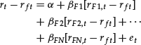
where
rt = return on the stock in month t
rft = the risk-free rate in month t
rFN,t = the return on factor N in month t
et = the error term for the stock in month t
α and βFN’s = parameters for the stock to be estimated by the regression model
t = month (t = 1, 2, … , T)
Thus, in order for a portfolio manager to build a portfolio or to compute portfolio risk measures using the above multifactor model for month T + 1, just as in the case of the characteristic line, some assumption about how to forecast the excess returns (i.e., rFN,T+1 − rf,T+1) for each factor is required.
Predictive Regressive Models
In the search for models to predict returns, predictive regressive models have been developed. To explain predictive regressive models, consider some stock return and an assumed number of predictors. These predicators could be financial measures and market measures. A predictive linear regressive model assumes that the stock return at any given time t is a weighted average of its predictors at an earlier time plus a constant and some error. Hence, the information needed for predicting a stock’s return does not require the forecasting of the predictor used in the regression model.
Predictive regressive models can also be defined by estimating a regression model where there are factors used as predictors at different lags. Such models, referred to as distributed lag models, have the advantage that they can capture the eventual dependence of returns not only on factors but also on the rate of change of factors. Here is the economic significance of such models. Suppose that a portfolio manager wants to create a predictive model based on, among other factors, “market sentiment.” In practice, market sentiment is typically measured as a weighted average of analysts’ forecasts. A reasonable assumption is that stock returns will be sensitive to the value of market sentiment but will be even more sensitive to changes in market sentiment. Hence, distributed lag models will be useful in this setting.
Linear Autoregressive Models
In a linear autoregressive model, a variable is regressed on its own past values. Past values are referred to as lagged values and when they are used as predictors in the model they are referred to as lagged variables. In the case of predictive return models, one of the lagged variables would be the past values of the return of the stock. If the model involves only the lagged variable of the stock return, it is called an autoregressive model (AR model). An AR model prescribes that the value of a variable at time t be a weighted average of the values of the same variable at times t – 1, t – 2, … , and so on (depending on number of lags) plus an error term. The weighting coefficients are the model parameters that must be estimated. If the model includes p lags, then p parameters must be estimated.
If there are other lagged variables in addition to the lagged variable representing the past values of the return on the stock included in the regression model, the model is referred to as a vector autoregressive model (VAR model). The model expresses each variable as a weighted average of its own lagged values plus the lagged values of the other variables. A VAR model with p lags is denoted by VAR(p) model. The benefit of a VAR model is that it can capture cross-autocorrelations; that is, a VAR model can model how values of a variable at time t are linked to the values of another variable at some other time. An important question is whether these links are causal or simply correlations.15
For a model to be useful, the number of parameters to be estimated needs to be small. In practice, the implementation of a VAR is complicated by the fact that such models can only deal with a small number of series. This is because when there is a large number of series—for example, the return processes for the individual stocks making up such aggregates as the S&P 500 Index—this would require a large number of parameters to be estimated. For example, if one wanted to model the daily returns of the S&P 500 with a VAR model that included two lags, the number of parameters to estimate would be 500,000. To have at least as many data points as parameters, one would need at least four years of data, or 1,000 trading days, for each stock return process, which is 1,000 × 500 = 500,000 data points. Under these conditions, estimates would be extremely noisy and the estimated model would be meaningless.
Dynamic Factor Models
Unlike a VAR model, which involves regressing returns on factors but does not model the factors, a dynamic factor model assumes factors follow a VAR model and returns (or prices) are regressed on these factors. The advantage of such models is that unlike the large amount of data needed to estimate the large number of parameters in a VAR model, a dynamic factor model can significantly reduce the number of parameters to be estimated and therefore the amount of data needed.
Hidden-Variable Models
Hidden-variable models attempt to represent states of the market using hidden variables. Probably the best known hidden-variable model is the autoregressive conditional heteroscedasticity (ARCH) and generalized autoregressive conditional heteroscedasticity (GARCH) family. ARCH/GARCH models use an autoregressive process to model the volatility of another process. The result is a rich representation of the behavior of the model volatility.
Another category of hidden-variable models is the Markov switching–vector autoregressive (MS–VAR) family. These models do allow forecasting of expected returns. The simplest MS–VAR model is the Hamilton model.16 In economics, this model is based on two random walk models—one with a drift for periods of economic expansion and the other with a smaller drift for periods of economic recession. The switch between the two models is governed by a probability transition table that prescribes the probability of switching from recession to expansion, and vice versa, and the probability of remaining in the same state.
IS FORECASTING MARKETS WORTH THE EFFORT?
In the end, all of this discussion leads to the question: What are the implications for portfolio managers and investors who are attempting or contemplating attempting building predictive return models? That is, how does this help portfolio managers and investors to decide if there is potentially sufficient benefit (i.e., trading profits and/or excess returns) in trying to extract information from market price data through quantitative modeling? There are three important points regarding this potential benefit.
The first, as stated by Fabozzi, Focardi, and Kolm (2006a, 11), is the following:
It is not true that progress in our ability to forecast will necessarily lead to a simplification in price and return processes. Even if investors were to become perfect forecasters, price and return processes might still exhibit complex patterns of forecastability in both expected values and higher moments, insofar as they might be martingales after dynamically adjusting for risk. No simple conclusion can be reached simply by assuming that investors are perfect forecasters: in fact, it is not true that the ability to forecast prices implies that prices are unpredictable random walks.
It is noteworthy that when the random walk hypothesis was first proposed in the academic community, it was the belief that the task of price forecasting efforts was a worthless exercise because prices were random walks. However, it seems reasonable to conclude that price processes will always be structured processes simply because investors are trying to forecast them. Modeling and sophisticated forecasting techniques will be needed to understand the risk-return trade-offs offered by the market.
The second point is that the idealized behavior of perfect forecasters does not have much to do with the actual behavior of real-world investors. The behavior of markets is the result, not of perfectly rational market agents, but of the action of market agents with limited intelligence, limited resources, and subject to unpredictable exogenous events. Consequently, the action of market agents is a source of uncertainty in itself. As a result, there is no theoretical reason to maintain that the multivariate random walk is the most robust model.
Real-world investors use relatively simple forecasting techniques such as linear regressions. It is reasonable to believe that when real-world investors employ judgment, there is the possibility of making large forecasting errors. As the behavioral finance camp argues, the preoccupation with the idealized behavior of markets populated by perfect forecasters seems to be misguided. Theorists who defend the assumption that investors in the real world are perfect forecasters, believe that it is unreasonable to assume that investors make systematic mistakes. Proponents of this assumption claim that, on average, investors make correct forecasts.
However, the evidence suggests that this claim is not true. Investors can make systematic mistakes and then hit some boundary, the consequences of which can be extremely painful in terms of wealth accumulation as we saw in the late 1990s with the bursting of the technology, media, and telecommunications bubble. As Fabozzi, Focardi, and Kolm (2006a, 11) conclude:
A pragmatic attitude prevails. Markets are considered to be difficult to predict but to exhibit rather complex structures that can be (and indeed are) predicted, either qualitatively or quantitatively.
Finally, an important point is that predictability is not the only path to profitability/excess returns. Citing once again from Fabozzi, Focardi, and Kolm (2006a, 11–12):
If prices behaved as simple models such as the random walk model or the martingale, they could nevertheless exhibit high levels of persistent profitability. This is because these models are characterized by a fixed structure of expected returns. Actually, it is the time-invariance of expected returns coupled with the existence of risk premiums that makes these models unsuitable as long-term models. … A model such as the geometric random walk model of prices leads to exponentially diverging expected returns. This is unrealistic in the long run, as it would lead to the concentration of all market capitalization in one asset. As a consequence, models such as the random walk model can only be approximate models over limited periods of time. This fact, in turn, calls attention to robust estimation methods. A random walk model is not an idealization that represents the final benchmark model: It is only a short-term approximation of what a model able to capture the dynamic feedbacks present in financial markets should be.
Hence, whether the random walk assumption is in fact the benchmark model of price processes must be addressed empirically. Yet, the view of portfolio managers is that markets offer patterns of predictability in returns, volatility (variance), and, possibly, higher moments. Because any such patterns might offer opportunities for realizing excess returns, a portfolio manager who ignores these patterns will be risking lost opportunities to enhance performance. As Fabozzi, Focardi, and Kolm (2006a, 24) state:
[S]imple random walk models with risk premiums are not necessarily the safest models. The joint assumptions that markets are unforecastable and that there are risk premiums is not necessarily the safest assumption.
KEY POINTS
- Despite the ongoing debate about the predictability of stock prices and returns, asset management firms have adopted statistical models of various levels of complexity for forecasting these values.
- The concept of forecastability rests on how one can forecast the future given the current information set known at that date.
- Prices or returns are said to be forecastable if the knowledge of the past influences our forecast of the future.
- The two beliefs that seem to be held in the investment community are (1) predictable processes allow investors to earn excess returns, and (2) unpredictable processes do not allow investors to earn excess returns.
- Predictable processes do not necessarily produce excess returns if they are associated with unfavorable risk, and unpredictable expectations can be profitable if the expected value is favorable.
- Probability theory is used in decision making to represent and measure the level of uncertainty.
- The absence of predictability means that the distribution of future returns does not change as a function of the present and past values of prices and returns.
- From this perspective, a price or return process is said to be predictable if its probability distributions depend on the current information set, and a price or return process is said to be unpredictable if its probability distributions do not vary over time. Using this concept of predictability, we can understand why prices and returns are difficult, perhaps even impossible, to predict.
- The key is that any prediction that might lead to an opportunity to generate a trading profit or an excess return tends to make that opportunity disappear. If stock return predictions are certain, then using simple arbitrage arguments would dictate that all stocks should have the same return. In fact, if stock returns could be predicted with certainty and if there were different returns, then investors would choose only those stocks with the highest returns.
- Because stock return forecasts are not certain, uncertain predictions are embodied in probability distributions.
- The problem faced by investors is whether general considerations of market efficiency are capable of determining the mathematical form of price or return processes. In particular, investors are interested in understanding if stock prices or returns are necessarily unpredictable.
- In solving this problem, the investor’s objective is to shun models that permit unreasonable inferences. The following solutions have been proposed: (1) Returns fluctuate randomly around a given mean (i.e., returns follow multivariate random walks); (2) returns are a fair game (i.e., returns are martingales); and (3) returns are a fair game after adjusting for risk.
- Concepts from probability theory and statistics that are relevant in understanding return forecasting models are conditional probability, conditional expectation, independent and identically distributed random variables, strict white noise, martingale difference sequence, white noise, error terms, and innovations.
- An arithmetic random walk, a martingale, and a strict arithmetic random walk describe the stochastic process for returns and prices. If stock prices or returns follow an arithmetic random walk, the mean is linearly unpredictable but higher moments might be predictable.
- In the case of a martingale, the mean is unpredictable (linearly and nonlinearly), although higher moments might be predictable.
- If stock prices or returns follow a strict random walk, the mean, variance, and higher moments are all unpredictable.
- The statistical-based predictive return models used by portfolio managers make conditional forecasts of expected returns using the current information set: past prices, company information, and financial market information. These models are classified as regressive models, linear autoregressive models, dynamic factor models, and hidden-variable models.
NOTES
1. See Bernstein (2008).
2. The contributions of Bachelier are too exhaustive (and technical) to describe here. In addition to his study of the behavior of prices, his work in the area of random walks predated Albert Einstein’s study of Brownian motion in physics by five years. His work in option pricing theory predated the well-known Black-Scholes option pricing model by 73 years.
3. See Samuelson (1965) and Fama (1965).
4. See Bernstein (1998) for an account of the development of the concepts of risk and uncertainty from the beginning of civilization to modern risk management.
5. The idea of probability as intensity of belief was introduced by Keynes (1921).
6. The idea of probability as a relative frequency was introduced by von Mises (1921).
7. See Rachev et al. (2007).
8. More specifically, the presence of autocorrelation does not bias the estimated parameters of the model but results in biases in the standard errors of the estimated parameters, which are used in testing the goodness of fit of the model.
9. Statements like this are intended as exemplifications but do not strictly embody sound econometric procedures. Adding lags has side effects, such as making estimations noisier, and cannot be used indiscriminately.
10. Fabozzi, Focardi, and Kolm (2006a, 66).
11. For a nontechnical discussion of these models, see Chapter 6 in Fabozzi, Focardi, and Kolm (2006a). For a more technical discussion see Fabozzi, Focardi, and Kolm (2006b).
12. For discussion of the merits and limits of AI from a practical perspective, see Leinweber and Beinart (1996).
13. Fabozzi, Focardi, and Kolm (2006a, 66).
14. See, for example, Fabozzi, Focardi, and Kolm (2006b).
15. For a discussion of the analysis of causality in VAR models, see Fabozzi, Focardi, and Kolm (2006b).
16. Hamilton (1989).
REFERENCES
Bachelier, L. (1900). Théorie de la spéculation. Annales Scientifiques de l’ École Normale Supérieure 3, 17: 21–86.
Bernstein, P. L. (1996). Against the Gods: The Remarkable Story of Risk. New York: John Wiley & Sons.
Bernstein, P. L. (2008). Are stock prices predictable? In Handbook of Finance, vol. 3, edited by F. J. Fabozzi (pp. 273–380). Hoboken, NJ: John Wiley & Sons.
Fabozzi, F. J., Focardi, S. M., and Kolm, P. N. (2006a). Trends in Quantitative Finance. Charlottesville, Va.: Research Foundation of the CFA Institute.
Fabozzi, F. J., Focardi, S. M., and Kolm, P. N. (2006b). Financial Modeling of the Equity Market: From CAPM to Cointegration. Hoboken, NJ: John Wiley & Sons.
Fama, E. F. (1965). The behavior of stock market prices. Journal of Business 38 (January): 34–105.
Hamilton, J. D. (1989). A new approach to the economic analysis of nonstationary time series and the business cycle. Econometrica 57, 2: 357–384.
Harrison, J. M., and Kreps, D. M. (1979). Martingales and arbitrage in multiperiod securities markets. Journal of Economic Theory 20: 381–408.
Harrison, J. M., and Pliska, S. R. (1981). Martingales and stochastic integrals in the theory of continuous trading. Stochastic Process Application 11: 215–260.
Harrison, J. M., and Pliska, S. R. (1985). A stochastic calculus model of continuous trading: Complete markets. Stochastic Process Application 15: 313–316.
Keynes, J. M. (1921). Treatise on Probability. London: Macmillan.
Leinweber, D. J., and Beinart, Y. (1996). Little AI goes a long way on Wall Street. Journal of Portfolio Management 27, 2: 95–106.
LeRoy, S. F. (1973). Risk aversion and the martingale property of stock prices. International Economic Review 14: 436–446.
Rachev, S. T., Hsu, J., Bagasheva B., and Fabozzi, F. J. (2008). Bayesian Methods in Finance. Hoboken, NJ: John Wiley & Sons.
Samuelson, P. A. (1965). Proof that properly anticipated prices fluctuate randomly. Industrial Management Review 6, 2: 41–50.
von Mises, R. (1928). Wahrscheinlichkeitsrechnung, Statisik und Wahrheit. Vienna: Julius Spring. (English edition translated in 1939 by J. Neyman, D. Scholl, and E. Rabinowitsch, Probability, Statistics and Truth. New York: Macmillan, 1939.)