Extracting Risk-Neutral Density Information from Options Market Prices

ARTURO LECCADITO, PhD

Business Administration Department, Università della Calabria

RADU TUNARU, PhD

Professor of Quantitative Finance, Business School, University of Kent

The concept of risk-neutral density (RND) plays an important theoretical role in asset pricing as outlined in Cox and Ross (1976), published very shortly after the publication of the Black-Scholes model. Since then, the estimation of RND has become an essential tool for central banks in monitoring the stability of the financial system and for measuring the impact of new policies. Investment banks also rely on the RND calibrated from liquid European vanilla options to determine the price of more exotic positions on their balance sheet that are not very liquid. Moreover, the first moments of the RND, such as implied volatility and skewness, can be used to design trading strategies.

One may argue that the information contained in option prices is redundant to the information provided by historical prices of the underlying asset. However, based on the 1987 stock market crash, Jackwerth and Rubinstein (1996) demonstrated that this is not the case. Prior to the crash, the RND estimated at one-month horizon had been close to lognormal but subsequently the shape of the RND changed considerably. At the same time, they also revealed that the historical distribution had been lognormal and it remained like that after the crash. In other words, the option prices in the equity market contain different information from the historical equity prices.

In this entry we highlight the main steps for estimating the RND associated with an equity index. We exemplify the estimation procedure by applying a model based on both the generalized inverse Gaussian distribution that has been advocated in the literature for financial modeling and the well-known lognormal mixture model that has been widely used by investment houses and central banks. These two models are straightforward and easy to apply since the option pricing formulas can be derived in closed form.

AN APPROPRIATE PARAMETRIC MODEL

The RND is recovered from a bundle of European vanilla call and put option prices on the same underlying asset X and with the same maturity T. The options differ in the exercise price K. Denoting with f(·) the probability density function of the underlying asset X under the risk-neutral probability measure , the European vanilla call price for strike K is

(1)

where r is the continuous compounding risk-free rate.

The partial derivative of 1 with respect to the strike price K

where F(·) is the cumulative distribution function under the risk-neutral measure. Thus

(2)

The RND probability function f can be obtained by derivation of the cumulative function F

(3)

One could then try to reconstruct either F or f from a grid of option prices using finite difference schemes. However, such numerical methods are notoriously unreliable and very sensitive to the sample of option prices available.

Over the years, two main classes of methods have emerged. First, parametric methods are underpinned by univariate distributions such as the Weibull distribution (see Savickas, 2002, 2005), the generalized beta distribution (see McDonald and Xu, 1995; Anagnou et al., 2005), the generalized lambda distribution (see Corrado, 2001), the generalized gamma distribution (see Albota et al., 2009), the g-and-h distribution as proposed by Dutta and Babbel (2005); and a mixture of univariate distributions such as that proposed by Gemmill and Saflekos (2000) for two lognormals, and Melick and Thomas (1997) for three lognormals.

The second class is defined by semiparametric and nonparametric methods such as (1) expansion methods as used by Jarrow and Rudd (1982) and Corrado and Su (1997), (2) direct fitting of the implied volatility curve with splines or other interpolation methods as described by Shimko (1993), Anagnou et al. (2003), and Brunner and Hafner (2003), (3) kernel methods developed in Ait-Sahalia and Lo (1998) and Ait-Sahalia and Duarte (2003), and (4) maximum entropy methods as applied by Buchen and Kelly (1996) and Avellaneda (1998).

The nonparametric approach usually requires a large sample of data in order to achieve a good fit. In financial markets, for many asset classes, large samples may simply not be available. In this entry, we focus on the fully parametric approach.

The strategy for parametric models represented by a vector of parameters θ is to minimize some type of discrepancy measure between the theoretical options prices and the observed market prices.

Given the availability of N European call options and M put options all with the same maturity T, the problem that must be solved is the minimization of the function

(4)

subject to the forward constraint , where F0 is the forward price on the same underlying asset X and the last term of the sum accounts for the forward martingale condition that must be satisfied for any parametric model. The notation Cmkt, and Pmkt, relates, respectively, to the actual option prices from the market. The function H is a discrepancy measure between the theoretical prices obtained under the chosen parametric RND f(·; θ) and the market prices.

While the H in (4) is widely used in practice, it is sometimes useful to consider other potential discrepancy measures such as

Since the market option prices that do not satisfy put-call parity are filtered out of the data used for calibration, it is possible to work with call prices only or with put prices only, if that is more convenient numerically.

TWO PARAMETRIC MODELS FOR RND ESTIMATION

In order to be able to reverse engineer the RND from options prices, a pricing formula for European vanilla options under the chosen distribution is needed. There is a great advantage in having the pricing formulas in closed form, otherwise numerical integral approximation methods must be employed and this means that there is a risk of introducing errors in the estimation procedure.

Here we illustrate the RND estimation procedure for two special cases, the general inverse Gaussian (GIG) distribution and the lognormal mixture (LnMix) distribution. For both models, closed-form solutions for pricing European options are available.

Pricing Options with the GIG Distribution

The GIG distribution has been advocated for applications in financial modeling due to its flexibility to fit heavy tails (see Bibby and Sorensen, 2003). The probability density function of the GIG distribution is1

(5)

where

is a normalizing constant that is related to the modified Bessel function of the third kind,

(6)

via

(7)

Further technical details on this distribution can be found in Paolella (2007).

The GIG distribution is well defined, or “proper,” for the parameter domain

Table 1 Call Option Prices on May 29, 1998, on the FTSE100 Index

There are also two boundary cases possible: (1) λ > 0, χ = 0 and ψ > 0 and (2) λ < 0, χ > 0 and ψ = 0. Applying some standard algebraic routine leads to

This formula can be rewritten in terms of the forward price as

(8)

RND Estimation with the LnMix Distribution

The importance of fat tails and non-normal distributions in modeling equity stock and vanilla options has become prominent in the aftermath of the Black Monday 1987 crisis. The LnMix model is a convex combination of several lognormal individual models. Bahra (1997) was the first to propose using the LnMix model for RND estimation. An exact solution for options pricing of vanilla European call and put options can be derived as a weighted sum of standard Black-Scholes prices. In practice, the preferred mixture model is the one based on two individual lognormal models.

If LN(x; α, β) is the lognormal distribution with parameters α and β, then the LnMix distribution is given by the following probability density function

(9)

Bahra (1997) described the formulas for pricing European vanilla call and put options

where

and N is the standard normal cumulative distribution function.

This model has five parameters α1, β1, α2, β2, and η and one should expect a better fit of data with this model compared to the GIG model that has only three parameters. If the calibration goodness-of-fit results are very similar between the two models, then the model with fewer parameters should be preferred based on the principle of parsimony.

Table 2 Discrepancy Measures across Maturities for the Data in Table 1

Figure 1 Absolute Percentage Errors for the First Four Maturities

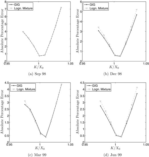
Figure 2 Absolute Percentage Errors for the Last Four Maturities

FITTING THE MODELS TO DATA

For the RND estimation with a parametric model, the main elements are (1) formulas for pricing either European call or European put options, together with a formula for the forward price, (2) a minimization procedure for a nonlinear function such as H1 in the function given by (4), and (3) a set of market option prices.

Here we illustrate the calibration of the GIG and LnMix models using a dataset reported in Table 1, which is described in Rebonato (2004, pp. 290--291), and it is a typical example for the UK equity market.

The goodness of fit of the two models can be assessed to some extent from the results in Table 2, which reports the values obtained for the sum of squared residual , where and m is the vector with components Kj/X0 reflecting moneyness. The smaller the value, the better is the fit. It is interesting that the GIG distribution, having three parameters, seems to calibrate across maturities very closely and is even a superior fit than the lognormal mixture (LnMix) model that uses five parameters.

A more informative comparison can be done by looking at the error structure versus moneyness. The fitting error for the two models and for each maturity are plotted in Figures 1 and 2 as the absolute percentage errors, defined for the European call option prices as 100 × , where is the same as the theoretical prices established in equation (1), which is calculated for the estimated parameter vector following the minimization procedure focused on the function given in (4). In the neighborhood of at-the-money prices, the absolute percentage error is less than 1%, while out-of-the-money or in-the-money, it may go even higher.

Which parametric model to use depends on the task at hand. It is possible that some parametric models perform better for some asset classes (such as foreign exchange), while other models perform better for different asset classes (such as equity). Some models may have a superior fit in the tails.

KEY POINTS

• The information contained in the risk-neutral density is useful to many participants in financial markets. Central banks use this information in monitoring the stability of the financial system and for assessing the impact of new policies, and banks use it for marking positions in exotic derivatives that they hold.
• To recover the RND, a bundle of market prices for European vanilla call and put options on the same underlying asset and with the same maturity is used.
• Parameteric and nonparametric models have been proposed for estimating the RND. For several reasons, in practice, parametric models are better to employ. The main elements of a parametric model to estimate RND are an option pricing formula combined with a forward price formula, a minimization procedure, and a database of observed option prices.
• RND estimation can be done easily with parametric models for which pricing formulas are available for European vanilla options. The generalized inverse Gaussian model and the lognormal mixture model are examples of such models.
• The calibration is done by minimizing a discrepancy measure between the theoretical model prices and the observed option market prices.

NOTE

1. IA(x) is the indicator function being equal to 1 when x A and zero otherwise.

REFERENCES

Ait-Sahalia, Y., and J. Duarte. (2003). Nonparametric option pricing under shape restrictions. Journal of Econometrics 116 : 9–47.

Ait-Sahalia, Y., and Lo, A. W. (1998). Nonparametric estimation of state-price densities implicit in financial asset prices. Journal of Finance 53: 499–547.

Albota, G., Fabozzi, F., and Tunaru, R. (2009). Estimating risk-neutral density with parametric models in interest rate markets. Quantitative Finance 9: 55–70.

Anagnou, I., Bedendo, M., Hodges, S., and Tompkins, R. (2005). The relation between implied and realized probability density functions. Review of Futures Markets 11: 41–66.

Avellaneda, M. (1998). Minimum-relative-entropy calibration of asset-pricing models. International Journal of Theoretical & Applied Finance 1: 447–472.

Bahra, B. (2007). Implied risk-neutral probability density functions from option prices: Theory and application. Report ISSN 1368-5562, Bank of England, London, EC2R 8AH.

Bibby, B. M., and Sorensen, M. (2003). Hyperbolic processes in finance. In Handbook of Heavy-Tailed Distributions in Finance, ed. S. T. Rachev. Chichester: Elsevier-North Holland, pp. 211–244.

Brunner, B., and Hafner, R. (2003). Arbitrage-free estimation of the risk-neutral density from the implied volatility smile. Journal of Computational Finance 7: 75–106.

Buchen, P. W., and Kelly, M. (1996). The maximum entropy distribution of an asset inferred from option prices. Journal of Financial & Quantitative Analysis 31: 143–159.

Corrado, C. J. (2001). Option pricing based on the generalized lambda distribution. Journal of Futures Markets 21: 213–236.

Corrado, C. J., and Su, T. (1997). Implied volatility skews and stock index skewness and kurtosis implied by S&P 500 index option prices. Journal of Derivatives 4: 8–19.

Cox, J., and Ross, S. (1976). The valuation of options for alternative stochastic processes. Journal of Financial Economics 3: 145–166.

Dutta, K. K., and Babbel, D. F. (2005). Extracting probabilistic information from the prices of interest rate options: Tests of distributional assumptions. Journal of Business 78: 841–870.

Gemmill, G., and Saflekos, G. (2000). How useful are implied distributions? Evidence from stock-index options. Journal of Derivatives 7: 83–98.

Jackwerth, J. C., and Rubinstein, M. (1996). Recovering probability distributions from options prices. Journal of Finance 51: 1611–1631.

Melick, W. R., and Thomas, C. P. (1997). Recovering an asset’s implied pdf from option prices: An application to crude oil during the Gulf crisis. Journal of Financial & Quantitative Analysis 32: 91–115.

Paolella, M. (2007). Intermediate Probability: A Computational Approach. Chichester: John Wiley & Sons.

Rebonato, R. (2004). Volatility and Correlation, 2nd ed., Chichester: John Wiley & Sons.

Savickas, R. (2005). Evidence on delta hedging and implied volatilities for the Black-Scholes, Gamma and Weibull option-pricing models. Journal of Financial Research 28: 299–317.

Shimko, D. (1993). Bounds of probability. RISK 6: 33–37.