Cross-Sectional Factor-Based Models and Trading Strategies

JOSEPH A. CERNIGLIA

Visiting Researcher, Courant Institute of Mathematical Sciences, New York University

PETTER N. KOLM, PhD

Director of the Mathematics in Finance Masters Program and Clinical Associate Professor Courant Institute of Mathematical Sciences, New York University

FRANK J. FABOZZI, PhD, CFA, CPA

Professor of Finance, EDHEC Business School

In the construction of factor models, factors are constructed from company characteristics and market data. In this entry, we explain and illustrate how to include multiple factors with the purpose of developing a dynamic multifactor trading strategy that incorporates a number of common institutional constraints such as turnover, transaction costs, sector, and tracking error. For this purpose, we use a combination of growth, value, quality, and momentum factors. For the purpose of our illustration, our universe of stocks is the Russell 1000 from December 1989 to December 2008, and we construct our factors by using the Compustat Point-In-Time and IBES databases. A complete list of the factors and data sets used is provided in the appendix.

We begin by reviewing several approaches for the evaluation of return premiums and risk characteristics to factors, including portfolio sorts, factor models, factor portfolios, and infor-mation coefficients. We then turn to techniques that are used to combine several factors into a single model—a trading strategy. In particular, we discuss the data driven, factor model, heuristic, and optimization approaches. It is critical to perform out-of-sample backtests of a trading strategy to understand its performance and risk characteristics. We cover the split-sample and recursive out-of-sample tests.

Throughout this entry, we provide a series of examples, including backtests of a multifactor trading strategy. The purpose of these examples is not to attempt to provide a profitable trading strategy, but rather to illustrate the process a financial modeler may follow when performing research. We emphasize that the factors that we use are well known and have for years been exploited by industry practitioners. We think that the value added of these examples is in the concrete illustration of the research and development process of a factor-based trading model.

CROSS-SECTIONAL METHODS FOR EVALUATION OF FACTOR PREMIUMS

There are several approaches used for the evaluation of return premiums and risk characteristics to factors. In this section, we discuss the four most commonly used approaches: portfolio sorts, factor models, factor portfolios, and information coefficients. We examine the methodology of each approach and summarize its advantages and disadvantages.

In practice, to determine the right approach for a given situation there are several issues to consider. One determinant is the structure of the financial data. A second determinant is the economic intuition underlying the factor. For example, sometimes we are looking for a monotonic relationship between returns and factors while at other times we care only about extreme values. A third determinant is whether the underlying assumptions of each approach are valid for the data-generating process at hand.

Portfolio Sorts

In the asset pricing literature, the use of portfolio sorts can be traced back to the earliest tests of the capital asset pricing model (CAPM). The goal of this particular test is to determine whether a factor earns a systematic premium. The portfolios are constructed by grouping together securities with similar characteristics (factors). For example, we can group stocks by market capitalization into 10 portfolios—from smallest to largest—such that each portfolio contains stocks with similar market capitalization. The next step is to calculate and evaluate the returns of these portfolios.

The return for each portfolio is calculated by equally weighting the individual stock returns. The portfolios provide a representation of how returns vary across the different values of a factor. By studying the return behavior of the factor portfolios, we may assess the return and risk profile of the factor. In some cases, we may identify a monotonic relationship of the returns across the portfolios. In other cases, we may identify a large difference in returns between the extreme portfolios. In still other cases, there may be no relationship between the portfolio returns. Overall, the return behavior of the portfolios will help us conclude whether there is a premium associated with a factor and describe its properties.

One application of the portfolio sort is the construction of a factor mimicking portfolio (FMP). An FMP is a long-short portfolio that goes long stocks with high values of a factor and short stocks with low values of a factor, in equal dollar amounts. An FMP is a zero-cost factor trading strategy.

Portfolio sorts have become so widespread among practitioners and academics alike that they elicit few econometric queries, and often no econometric justification for the technique is offered. While a detailed discussion of these topics is beyond the scope of this book, we would like to point out that asset pricing tests used on sorted portfolios may exhibit a bias that favors rejecting the asset pricing model under consideration.1

The construction of portfolios sorted on a factor is straightforward:

• Choose an appropriate sorting methodology.
• Sort the assets according to the factor.
• Group the sorted assets into N portfolios (usually N = 5, or N = 10).
• Compute average returns (and other statistics) of the assets in each portfolio over subsequent periods.

The standard statistical testing procedure for portfolio sorts is to use a Student’s t-test to evaluate the significance of the mean return differential between the portfolios of stocks with the highest and lowest values of the factor.

Choosing the Sorting Methodology

The sorting methodology should be consistent with the characteristics of the distribution of the factor and the economic motivation underlying its premium. We list six ways to sort factors:

Method 1

• Sort stocks with factor values from the highest to lowest.

Method 2

• Sort stocks with factor values from the lowest to highest.

Method 3

• First allocate stocks with zero factor values into the bottom portfolio.
• Sort the remaining stocks with nonzero factor values into the remaining portfolios.

For example, the dividend yield factor would be suitable for this sorting approach. This approach aligns the factor’s distributional characteristics of dividend and nondividend-paying stocks with the economic rationale. Typically, nondividend-paying stocks maintain characteristics that are different from dividend paying stocks. So we group nondividend-paying stocks into one portfolio. The remaining stocks are then grouped into portfolios depending on the size of their nonzero dividend yields. We differentiate among stocks with dividend yield because of two reasons: (1) the size of the dividend yield is related to the maturity of the company, and (2) some investors prefer to receive their investment return as dividends.

Method 4

• Allocate stocks with zero factor values into the middle portfolio.
• Sort stocks with positive factor values into the remaining higher portfolios (greater than the middle portfolio).
• Sort stocks with negative factor values into the remaining lower portfolios (less than the middle portfolio).

Method 5

• Sort stocks into partitions.
• Rank assets within each partition.
• Combine assets with the same ranking from the different partitions into portfolios.

An example will clarify this procedure. Suppose we want to rank stocks according to earnings growth on a sector-neutral basis. First, we separate stocks into groups corresponding to their sector. Within each sector, we rank the stocks according to their earnings growth. Lastly, we group all stocks with the same rankings of earnings growth into the final portfolio. This process ensures that each portfolio will contain an equal number of stocks from every sector, thereby the resulting portfolios are sector neutral.

Figure 1 Portfolio Sorts Based on the EBITDA/EV Factor

Method 6

• Separate all the stocks with negative factor values. Split the group of stocks with negative values into two portfolios using the median value as the break point.
• Allocate stocks with zero factor values into one portfolio.
• Sort the remaining stocks with nonzero factor values into portfolios based on their factor values.

An example of method 6 is the share repurchase factor. We are interested in the extreme positive and negative values of this factor. As we see in Figure 5(A), the distribution of these factors is leptokurtic with the positive values skewed to the right and the negative values clustered in a small range. By choosing method 6 to sort this variable, we can distinguish between those values we view as extreme. The negative values are clustered so we want to distinguish among the magnitudes of those values. We accomplish this because our sorting method separates the negative values by the median of the negative values. The largest negative values form the extreme negative portfolio. The positive values are skewed to the right, so we want to differentiate between the larger and smaller positive values. When implementing portfolio method 6, we would also separate the zero values from the positive values.

The portfolio sort methodology has several advantages. The approach is easy to implement and can easily handle stocks that drop out or enter into the sample. The resulting portfolios diversify away idiosyncratic risk of individual assets and provide a way of assessing how average returns differ across different magnitudes of a factor.

The portfolio sort methodology has several disadvantages. The resulting portfolios may be exposed to different risks beyond the factor the portfolio was sorted on. In those instances, it is difficult to know which risk characteristics have an impact on the portfolio returns. Because portfolio sorts are nonparametric, they do not give insight as to the functional form of the relation between the average portfolio returns and the factor.

Next we provide three examples to illustrate how the economic intuition of the factor and cross-sectional statistics can help determine the sorting methodology.

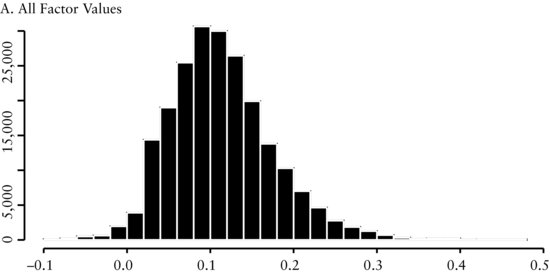
Example 1: Portfolio Sorts Based on the EBITDA/EV Factor

Panel A of Figure 1 contains the cross-sectional distribution of the EBITDA/EV factor. This distribution is approximately normally distributed around a mean of 0.1, with a slight right skew. We use method 1 to sort the variables into five portfolios (denoted by q1, …, q5) because this sorting method aligns the cross-sectional distribution of factor returns with our economic intuition that there is a linear relationship between the factor and subsequent return. In Figure 1(B), we see that there is a large difference between the equally weighted monthly returns of portfolio 1 (q1) and portfolio 5 (q5). Therefore, a trading strategy (denoted by ls in the graph) that goes long portfolio 1 and short portfolio 5 appears to produce abnormal returns.

Figure 2 The Revisions Factor

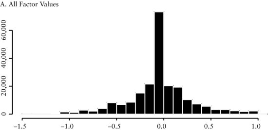
Example 2: Portfolio Sorts Based on the Revisions Factor

In Figure 2(A), we see that the distribution of earnings revisions is leptokurtic around a mean of about zero, with the remaining values symmetrically distributed around the peak. The pattern in this cross-sectional distribution provides insight on how we should sort this factor. We use method 3 to sort the variables into five portfolios. The firms with no change in revisions we allocate to the middle portfolio (portfolio 3). The stocks with positive revisions we sort into portfolios 1 and 2, according to the size of the revisions—while we sort stocks with negative revisions into portfolios 4 and 5, according to the size of the revisions. In Figure 2(B), we see there is a relationship between the portfolios and subsequent monthly returns. The positive relationship between revisions and subsequent returns agrees with the factor’s underlying economic intuition: We expect that firms with improving earnings should outperform. The trading strategy that goes long portfolio 1 and short portfolio 5 (denoted by ls in the graph) appears to produce abnormal returns.

Figure 3 The Share Repurchase Factor

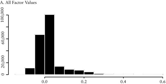
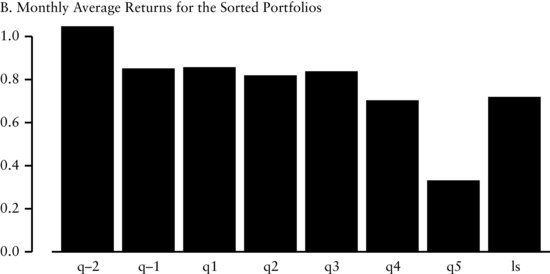
Example 3: Portfolio Sorts Based on the Share Repurchase Factor

In Figure 3(A), we see the distribution of share repurchase is asymmetric and leptokurtic around a mean of zero. The pattern in this cross-sectional distribution provides insight on how we should sort this factor. We use method 6 to sort the variables into seven portfolios. We group stocks with positive revisions into portfolios 1 through 5 (denoted by q1, …, q5 in the graph) according to the magnitude of the share repurchase factor. We allocate stocks with negative repurchases into portfolios q−2 and q−1 where the median of the negative values determines their membership. We split the negative numbers because we are interested in large changes in the shares outstanding. In Figure 3(B), unlike the other previous factors, we see that there is not a linear relationship between the portfolios. However, there is a large difference in return between the extreme portfolios (denoted by ls in the graph). This large difference agrees with the economic intuition of this factor. Changes in the number of shares outstanding are a potential signal for the future value and prospects of a firm. On the one hand, a large increase in shares outstanding may signal to investors (1) the need for additional cash because of financial distress, or (2) that the firm may be overvalued. On the other hand, a large decrease in the number of shares outstanding may indicate that management believes the shares are undervalued. Finally, small changes in shares outstanding, positive or negative, typically do not have an impact on stock price and therefore are not significant.

Information Ratios for Portfolio Sorts

The information ratio (IR) is a statistic for summarizing the risk-adjusted performance of an investment strategy. It is defined as the ratio of the average excess return to the standard deviation of return. For actively managed equity long portfolios, the IR measures the risk-adjusted value a portfolio manager is adding relative to a benchmark.2 IR can also be used to capture the risk-adjusted performance of long-short portfolios from portfolio sorts. When comparing portfolios built using different factors, the IR is an effective measure for differentiating the performance between the strategies.

New Research on Portfolio Sorts

As we mentioned earlier in this section, the standard statistical testing procedure for portfolio sorts is to use a Student’s t-test to evaluate the mean return differential between the two portfolios containing stocks with the highest and lowest values of the sorting factor. However, evaluating the return between these two portfolios ignores important information about the overall pattern of returns among the remaining portfolios.

Recent research by Patton and Timmermann (2009) provides new analytical techniques to increase the robustness of inference from portfolio sorts. The technique tests for the presence of a monotonic relationship between the portfolios and their expected returns. To find out if there is a systematic relationship between a factor and portfolio returns, they use the monotonic relation (MR) test to reveal whether the null hypothesis of no systematic relationship can be rejected in favor of a monotonic relationship predicted by economic theory. By MR it is meant that the expected returns of a factor should rise or decline monotonically in one direction as one goes from one portfolio to another. Moreover, Patton and Timmermann develop separate tests to determine the direction of deviations in support of or against the theory.

The authors emphasize several advantages in using this approach. The test is nonparametric and applicable to other cases of portfolios such as two-way and three-way sorts. This test is easy to implement via bootstrap methods. Furthermore, this test does not require specifying the functional form (e.g., linear) in relating the sorting variable to expected returns.

FACTOR MODELS

Classical financial theory states that the average return of a stock is the payoff to investors for taking on risk. One way of expressing this risk-reward relationship is through a factor model. A factor model can be used to decompose the returns of a security into factor-specific and asset-specific returns

where βi,1, βi,2, …, βi,K are the factor exposures of stock i, f1,t, f2,t, …, fK,t are the factor returns, αi is the average abnormal return of stock i, and εi,t is the residual.

This factor model specification is contemporaneous, that is, both left- and right-hand side variables (returns and factors) have the same time subscript, t. For trading strategies one generally applies a forecasting specification where the time subscript of the return and the factors are t + h (h ≥ 1) and t, respectively. In this case, the econometric specification becomes

How do we interpret a trading strategy based on a factor model? The explanatory variables represent different factors that forecast security returns, and each factor has an associated factor premium. Therefore, future security returns are proportional to the stock’s exposure to the factor premium

and the variance of future stock return is given by

where and and .

In the next section we discuss some specific econometric issues regarding cross-sectional regressions and factor models.

Econometric Considerations for Cross-Sectional Factor Models

In cross-sectional regressions, where the dependent variable3 is a stock’s return and the independent variables are factors, inference problems may arise that are the result of violations of classical linear regression theory. The three most common problems are measurement problems, common variations in residuals, and multicollinearity.

Measurement Problems

Some factors are not explicitly given, but need to be estimated. These factors are estimated with an error. This error can have an impact on the inference from a factor model. This problem is commonly referred to as the “errors in variables problem.” For example, a factor that is comprised of a stock’s beta is estimated with an error because beta is determined from a regression of stock excess returns on the excess returns of a market index. While beyond the scope of this entry, several approaches have been suggested to deal with this problem.4

Common Variation in Residuals

The residuals from a regression often contain a source of common variation. Sources of common variation in the residuals are heteroskedasticity and serial correlation.5 We note that when the form of heteroskedasticity and serial correlation is known, we can apply generalized least squares (GLS). If the form is not known, it has to be estimated, for example as part of feasible generalized least squares (FGLS). We summarize some additional possibilities next.

Heteroskedasticity occurs when the variance of the residual differs across observations and affects the statistical inference in a linear regression. In particular, the estimated standard errors will be underestimated and the t-statistics will therefore be inflated. Ignoring heteroskedasticity may lead the researcher to find significant relationships where none actually exist. Several procedures have been developed to calculate standard errors that are robust to heteroskedasticity, also known as heteroskedasticity-consistent standard errors.

Serial correlation occurs when residuals terms in a linear regression are correlated, violating the assumptions of regression theory. If the serial correlation is positive, then the standard errors are underestimated and the t-statistics will be inflated. Cochrane (2005) suggests that the errors in cross-sectional regressions using financial data are often off by a factor of 10. Procedures are available to correct for serial correlation when calculating standard errors.

When the residuals from a regression are both heteroskedastic and serially correlated, procedures are available to correct them. One commonly used procedure is the one proposed by Newey and West (1987) referred to as the “Newey-West corrections,” and its extension by Andrews (1991).

Petersen (2009) provides guidance on choosing the appropriate method to use for correctly calculating standard errors in panel data regressions when the residuals are correlated. He shows the relative accuracy of the different methods depends on the structure of the data. In the presence of firm effects, where the residuals of a given firm may be correlated across years, ordinary least squares (OLS), Newey-West (modified for panel data sets), or Fama-MacBeth,6 corrected for first-order autocorrelation, all produce biased standard errors. To correct for this, Petersen recommends using standard errors clustered by firms. If the firm effect is permanent, the fixed effects and random effects models produce unbiased standard errors. In the presence of time effects, where the residuals of a given period may be correlated across difference firms (cross-sectional dependence), Fama-MacBeth produces unbiased standard errors. Furthermore, standard errors clustered by time are unbiased when there are a sufficient number of clusters. To select the correct approach he recommends determining the form of dependence in the data and comparing the results from several methods.

Gow, Ormazabal, and Taylor (2009) evaluate empirical methods used in accounting research to correct for cross-sectional and time-series dependence. They review each of the methods, including several methods from the accounting literature that have not previously been formally evaluated, and discuss when each methods produces valid inferences.

Multicollinearity

Multicollinearity occurs when two or more independent variables are highly correlated. We may encounter several problems when this happens. First, it is difficult to determine which factors influence the dependent variable. Second, the individual p values can be misleading—a p value can be high even if the variable is important. Third, the confidence intervals for the regression coefficients will be wide. They may even include zero. This implies that we cannot determine whether an increase in the independent variable is associated with an increase—or a decrease—in the dependent variable. There is no formal solution based on theory to correct for multicollinearity. The best way to correct for multicollinearity is by removing one or more of the correlated independent variables. It can also be reduced by increasing the sample size.

Fama-MacBeth Regression

To address the inference problem caused by the correlation of the residuals, Fama and MacBeth (1973) proposed the following methodology for estimating cross-sectional regressions of returns on factors. For notational simplicity, we describe the procedure for one factor. The multifactor generalization is straightforward.

First, for each point in time t we perform a cross-sectional regression:

In the academic literature, the regressions are typically performed using monthly or quarterly data, but the procedure could be used at any frequency.

The mean and standard errors of the time series of slopes and residuals are evaluated to determine the significance of the cross-sectional regression. We estimate f and εi as the average of their cross-sectional estimates, therefore,

The variations in the estimates determine the standard error and capture the effects of residual correlation without actually estimating the correlations.7 We use the standard deviations of the cross-sectional regression estimates to calculate the sampling errors for these estimates

Cochrane (2005) provides a detailed analysis of this procedure and compares it to cross-sectional OLS and pooled time-series cross-sectional OLS. He shows that when the factors do not vary over time and the residuals are cross-sectionally correlated, but not correlated over time, then these procedures are all equivalent.

Information Coefficients

To determine the forecast ability of a model, practitioners commonly use a statistic called the information coefficient (IC). The IC is a linear statistic that measures the cross-sectional correlation between a factor and its subsequent realized return:8

where ft is a vector of cross sectional factor values at time t and rt,t+k is a vector of returns over the time period t to t + k.

Just like the standard correlation coefficient, the values of the IC range from −1 to +1. A positive IC indicates a positive relation between the factor and return. A negative IC indicates a negative relation between the factor and return. ICs are usually calculated over an interval, for example, daily or monthly. We can evaluate how a factor has performed by examining the time series behavior of the ICs. Looking at the mean IC tells how predictive the factor has been over time.

An alternate specification of this measure is to make ft the rank of a cross-sectional factor. This calculation is similar to the Spearman rank coefficient. By using the rank of the factor, we focus on the ordering of the factor instead of its value. Ranking the factor value reduces the undue influence of outliers and reduces the influence of variables with unequal variances. For the same reasons, we may also choose to rank the returns instead of using their numerical value.

Sorensen, Qian, and Hua (2007) present a framework for factor analysis based on ICs. Their measure of IC is the correlation between the factor ranks, where the ranks are the normalized z-score of the factor,9 and subsequent return. Intuitively, this IC calculation measures the return associated with a one standard deviation exposure to the factor. Their IC calculation is further refined by risk adjusting the value. To risk adjust, the authors remove systematic risks from the IC and accommodate the IC for specific risk. By removing these risks, Qian and Hua (2004) show that the resulting ICs provide a more accurate measure of the return forecasting ability of the factor.

The subsequent realized returns to a factor typically vary over different time horizons. For example, the return to a factor based on price reversal is realized over short horizons, while valuation metrics such as EBITDA/EV are realized over longer periods. It therefore makes sense to calculate multiple ICs for a set of factor forecasts whereby each calculation varies the horizon over which the returns are measured.

The IC methodology has many of the same advantages as regression models. The procedure is easy to implement. The functional relationship between factor and subsequent returns is known (linear).

ICs can also be used to assess the risk of factors and trading strategies. The standard deviation of the time series (with respect to t) of ICs for a particular factor (std(ICt,t+k)) can be interpreted as the strategy risk of a factor. Examining the time series behavior of std(ICt,t+k) over different time periods may give a better understanding of how often a particular factor may fail. Qian and Hua show that std(ICt,t+k) can be used to more effectively understand the active risk of investment portfolios. Their research demonstrates that ex post tracking error often exceeds the ex ante tracking provided by risk models. The difference in tracking error occurs because tracking error is a function of both ex ante tracking error from a risk model and the variability of information coefficients, std(ICt,t+k). They define the expected tracking error as

where N is the number of stocks in the universe (breath), σmodel is the risk model tracking error, and dis(Rt) is dispersion of returns10 defined by

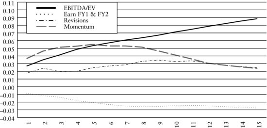
Figure 4 Information Coefficients over Various Horizons for EBITDA/EV, Growth of Fiscal Year 1 and Fiscal Year 2 Earnings Estimates, Revisions, and Momentum Factors

Example: Information Coefficients

Figure 4 displays the time-varying behavior of ICs for each one of the factors EBITDA/EV, growth of fiscal year 1 and fiscal year 2 earnings estimates, revisions, and momentum. The graph shows the time series average of information coefficients:

The graph depicts the information horizons for each factor, showing how subsequent return is realized over time. The vertical axis shows the size of the average information coefficient for k = 1, 2, …, 15.

Specifically, the EBITDA/EV factor starts at almost 0.03 and monotonically increases as the investment horizon lengthens from one month to 15 months. At 15 months, the EBITDA/EV factor has an IC of 0.09, the highest value among all the factors presented in the graph. This relationship suggests that the EBITDA/EV factor earns higher returns as the holding period lengthens.

The other ICs of the factors in the graph are also interesting. The growth of fiscal year 1 and fiscal year 2 earnings estimates factor is defined as the growth in current fiscal year (fy1) earnings estimates to the next fiscal year (fy2) earnings estimates provided by sell-side analysts.11 We call the growth of fiscal year 1 and fiscal year 2 earnings estimates factor the earnings growth factor throughout the remainder of the entry. The IC is negative and decreases as the investment horizon lengthens. The momentum factor starts with a positive IC of 0.02 and increases to approximately 0.055 in the fifth month. After the fifth month, the IC decreases. The revisions factor starts with a positive IC and increases slightly until approximately the eleventh month at which time the factor begins to decay.

Looking at the overall patterns in the graph, we see that the return realization pattern to different factors varies. One notable observation is that the returns to factors don’t necessarily decay but sometimes grow with the holding period. Understanding the multiperiod effects of each factor is important when we want to combine several factors. This information may influence how one builds a model. For example, we can explicitly incorporate this information about information horizons into our model by using a function that describes the decay or growth of a factor as a parameter to be calibrated. Implicitly, we could incorporate this information by changing the holding period for a security traded for our trading strategy. Specifically, Sneddon (2008) discusses an example that combines one signal that has short-range predictive power with another that has long-range power. Incorporating this information about the information horizon often improves the return potential of a model. Kolm (2010) describes a general multiperiod model that combines information decay, market impact costs, and real world constraints.

Factor Portfolios

Factor portfolios are constructed to measure the information content of a factor. The objective is to mimic the return behavior of a factor and minimize the residual risk. Similar to portfolio sorts, we evaluate the behavior of these factor portfolios to determine whether a factor earns a systematic premium.

Typically, a factor portfolio has a unit exposure to a factor and zero exposure to other factors. Construction of factor portfolios requires holding both long and short positions. We can also build a factor portfolio that has exposure to multiple attributes, such as beta, sectors, or other characteristics. For example, we could build a portfolio that has a unit exposure to book-to-price and small size stocks. Portfolios with exposures to multiple factors provide the opportunity to analyze the interaction of different factors.

A Factor Model Approach

By using a multifactor model, we can build factor portfolios that control for different risks.12 We decompose return and risk at a point in time into a systematic and specific component using the regression:

where r is an N vector of excess returns of the stocks considered, X is an N by K matrix of factor loadings, b is a K vector of factor returns, and u is an N vector of firm specific returns (residual returns). Here, we assume that factor returns are uncorrelated with the firm specific return. Further assuming that firm specific returns of different companies are uncorrelated, the N by N covariance matrix of stock returns V is given by

where F is the K by K factor return covariance matrix and Δ is the N by N diagonal matrix of variances of the specific returns.

We can use the Fama-MacBeth procedure discussed earlier to estimate the factor returns over time. Each month, we perform a GLS regression to obtain

OLS would give us an unbiased estimate, but since the residuals are heteroskedastic the GLS methodology is preferred and will deliver a more efficient estimate. The resulting holdings for each factor portfolio are given by the rows of .

An Optimization-Based Approach

A second approach to build factor portfolios uses mean-variance optimization. Using optimization techniques provides a flexible approach for implementing additional objectives and constraints.13

Figure 5 Results from Portfolio Sorts

Using the notation from the previous subsection, we denote by X the set of factors. We would like to construct a portfolio that has maximum exposure to one target factor from X (the alpha factor), zero exposure to all other factors, and minimum portfolio risk. Let us denote the alpha factor by Xα and all the remaining ones by Xσ. Then the resulting optimization problem takes the form

The analytical solution to this optimization problem is given by

We may want to add additional constraints to the problem. Constraints are added to make factor portfolios easier to implement and meet additional objectives. Some common constraints include limitations on turnover, transaction costs, the number of assets, and liquidity preferences. These constraints14 are typically implemented as linear inequality constraints. When no analytical solution is available to solve the optimization with linear inequality constraints, we have to resort to quadratic programming (QP).15

PERFORMANCE EVALUATION OF FACTORS

Analyzing the performance of different factors is an important part of the development of a factor-based trading strategy. A researcher may construct and analyze over a hundred different factors, so a process to evaluate and compare these factors is needed. Most often this process starts by trying to understand the time-series properties of each factor in isolation and then study how they interact with each other.

To give a basic idea of how this process may be performed, we use the five factors introduced earlier in this entry: EBITDA/EV, revisions, share repurchase, momentum, and earnings growth. These are a subset of the factors that we use in the factor trading strategy model discussed later in the entry. We choose a limited number of factors for ease of exposition. In particular, we emphasize those factors that possess more interesting empirical characteristics.

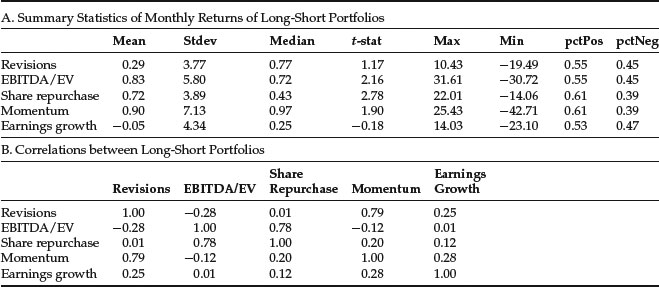
Figure 5(A) presents summary statistics of monthly returns of long-short portfolios constructed from these factors. We observe that the average monthly return ranges from −0.05% for the earnings growth to 0.90% for the momentum factor. The t-statistics for the mean return are significant at the 95% level for the EBITDA/EV, share repurchase, and momentum factors. The monthly volatility ranges from 3.77% for the revisions factor to 7.13% for the momentum factor. In other words, the return and risk characteristics among factors vary significantly. We note that the greatest monthly drawdown has been large to very large for all of the factors, implying significant downside risk. Overall, the results suggest that there is a systematic premium associated with the EBITDA/EV, share repurchase, and momentum factors.

Figure 6 Cumulative Returns of Long-Short Portfolios

Let pctPos and pctNeg denote the fraction of positive and negative returns over time, respectively. These measures offer another way of interpreting the strength and consistency of the returns to a factor. For example, EBITDA/EV and momentum have t-statistics of 2.16 and 1.90, respectively, indicating that the former is stronger. However, pctPos (pctNeg) are 0.55 versus 0.61 (0.45 versus 0.39) showing that positive returns to momentum occur more frequently. This may provide reassurance of the usefulness of the momentum factor, despite the fact that its t-statistic is below the 95% level.

Figure 5(B) presents unconditional correlation coefficients of monthly returns for long-short portfolios. The comovement of factor returns varies among the factors. The lowest correlation is −0.28 between EBITDA/EV and revisions. The highest correlation is 0.79 between momentum and revisions. In addition, we observe that the correlation between revisions and share repurchase, and between EBITDA/EV and earnings growth are close to zero. The broad range of correlations provides evidence that combining uncorrelated factors could produce a successful strategy.

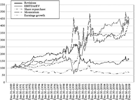
Figure 6 presents the cumulative returns for the long-short portfolios. The returns of the long-short factor portfolios experience substantial volatility. We highlight the following patterns of cumulative returns for the different factors:

Figure 7 Summary of Monthly Factor Information Coefficients

• The cumulative return of the revisions factor is positive in the early periods (12/1989 to 6/1998). While it is volatile, its cumulative return is higher in the next period (7/1998 to 7/2000). It deteriorates sharply in the following period (8/2000 to 6/2003), and levels out in the later periods (7/2003 to 12/2008).
• The performance of the EBITDA/EV factor is consistently positive in the early periods (12/1989 to 9/1998), deteriorates in the next period (10/1998 to 1/2000) and rebounds sharply (2/2000 to 7/2002), grows at a slower but more historically consistent rate in the later periods (8/2002 to 4/2007), deteriorates in the next period (5/2007 to 9/2007), and returns to more historically consistent returns in last period (10/2007 to 12/2008).
• The cumulative return of the share repurchase factor grows at a slower pace in the early years (12/1989 to 5/1999), falls slightly in the middle periods (6/1999 to 1/2000), rebounds sharply (2/2000 to 7/2002), falls then flattens out in the next period (8/2002 to 4/2008), and increases at a large rate late in the graph (5/2008 to 12/2008).
• The momentum factor experiences the largest volatility. This factor performs consistently well in the early period (12/1989 to 12/1998), experiences sharp volatility in the middle period (1/1999 to 5/2003), flattens out (6/2003 to 6/2007), and grows at an accelerating rate from (7/2007 to 12/2008).
• The performance of the earnings growth factor is flat or negative throughout the entire period.

The overall pattern of the cumulative returns among the factors clearly illustrates that factor returns and correlations are time varying.

In Figure 7(A), we present summary statistics of the monthly information coefficients of the factors. The average monthly information coefficients range from 0.03 for EBITDA/EV and momentum, to 0.01 for the share repurchase factor. The t-statistics for the mean ICs are significant at the 95% level for all factors except earnings growth. With the exception of share repurchase and earnings growth, the fraction of positive returns of the factors are significantly greater than that of the negative returns.

The share repurchase factor requires some comments. The information coefficient is negative, in contrast to the positive return in the long-short portfolio sorts, because negative share repurchases are correlated with subsequent return. The information coefficient is lower than we would expect because there is not a strong linear relation between the return and the measures. As the results from the portfolio sorts indicate, the extreme values of this factor provide the highest returns.

Figure 7(B) displays unconditional correlation coefficients of the monthly information coefficients. The comovement of the ICs factor returns varies among the factors. The lowest correlation is −0.66 between EBITDA/EV and share repurchases. But again this should be interpreted with caution because it is negative repurchases that we view as attractive. The highest correlation reported in the exhibit is 0.79 between momentum and revisions. Similar to the correlation of long-short factor portfolio returns, the diverse set of correlations provides evidence that combining uncorrelated factors may produce a successful strategy.

In Figure 8(A), we present summary statistics of the time series average of the monthly coefficients from the Fama-MacBeth (FM) regressions of the factors. The information provided by the FM coefficients differs from the information provided by portfolio sorts. The FM coefficients show the linear relationship between the factor and subsequent returns, while the results from the portfolio sorts provide information on the extreme values of the factors and subsequent returns. The difference in the size of the mean returns between the FM coefficients and portfolio sorts exits partially because the intercept terms from the FM regressions are not reported in the exhibit.

Figure 8 Summary of Monthly Fama-MacBeth Regression Coefficients

The average monthly FM coefficient ranges from −0.18 for share repurchase to 0.31 for the momentum factor. Again the share repurchase results should be interpreted with caution because it is negative repurchases that we view as attractive. The t-statistics are significant at the 95% level for the EBITDA/EV and share repurchase factors.

Also, we compare the results of portfolio sorts in Figure 7(A) with the FM coefficients in Figure 8(A). The rank ordering of the magnitude of factor returns is similar between the two panels. The t-statistics are slightly higher in the FM regressions than the portfolio sorts. The correlation coefficients for the portfolio sorts in Figure 7(B) are consistent with the FM coefficients in Figure 8(B) for all the factors except for shares repurchases. The results for share repurchases need to be interpreted with caution because it is negative repurchases that we view as attractive. The portfolio sorts take that into account while FM regressions do not.

To better understand the time variation of the performance of these factors, we calculate rolling 24-month mean returns and correlations of the factors. The results are presented in Figure 9. We see that the returns and correlations to all factors are time varying. A few of the time series experience large volatility in the rolling 24-month returns. The EBITDA/EV factor shows the largest variation followed by the momentum and share repurchase factors. All factors experience periods where the rolling average returns are both positive and negative.

Figure 10 presents the rolling correlation between pairs of the factors. There is substantial variability in many of the pairs. In most cases the correlation moves in a wave-like pattern. This pattern highlights the time-varying property of the correlations among the factors. This property will be important to incorporate in a factor trading model. The most consistent correlation is between momentum and revisions factors and this correlation is, in general, fairly high.

Figure 9 Rolling 24-Month Mean Returns for the Factors

Figure 10 Rolling 24-Month Correlations of Monthly Returns for the Factors

MODEL CONSTRUCTION METHODOLOGIES FOR A FACTOR-BASED TRADING STRATEGY

In the previous section, we analyzed the performance of each factor. The next step in building our trading strategy is to determine how to combine the factors into one model. The key aspect of building this model is to (1) determine what factors to use out of the universe of factors that we have, and (2) how to weight them.

We describe four methodologies to combine and weight factors to build a model for a trading strategy. These methodologies are used to translate the empirical work on factors into a working model. Most of the methodologies are flexible in their specification and there is some overlap between them. Though the list is not exhaustive, we highlight those processes frequently used by quantitative portfolio managers and researchers today. The four methodologies are the data driven, the factor model, the heuristic, and the optimization approaches.

It is important to be careful how each methodology is implemented. In particular, it is critical to balance the iterative process of finding a robust model with good forecasting ability versus finding a model that is a result of data mining.

The Data Driven Approach

A data driven approach uses statistical methods to select and weight factors in a forecasting model. This approach uses returns as the independent variables and factors as the dependent variables. There are a variety of estimation procedures, such as neural nets, classification trees, and principal components, that can be used to estimate these models. Usually a statistic is established to determine the criteria for a successful model. The algorithm of the statistical method evaluates the data and compares the results against the criteria.

Many data driven approaches have no structural assumptions on potential relationships the statistical method finds. Therefore, it is sometimes difficult to understand or even explain the relationship among the dependent variables used in the model.

Deistler and Hamann (2005) provide an example of a data driven approach to model development. The model they develop is used for forecasting the returns to financial stocks. To start, they split their data sample into two parts—an in-sample part for building the model and an out-of-sample part to validate the model. They use three different types of factor models for forecasting stock returns: quasistatic principal components, quasistatic factor models with idiosyncratic noise, and reduced rank regression. For model selection Deistler and Hamann use an iterative approach where they find the optimal mix of factors based on the Akaike’s information criterion and the Bayesian information criterion. A large number of different models are compared using the out-of-sample data. They find that the reduced rank model provides the best performance. This model produced the highest out-of-sample R2s, hit rates,16 and Diebold-Mariano test statistic17 among the different models evaluated.

The Factor Model Approach

In this section, we briefly address the use of factor models for forecasting. The goal of the factor model is to develop a parsimonious model that forecasts returns accurately. One approach is for the researcher to predetermine the variables to be used in the factor model based on economic intuition. The model is estimated and then the estimated coefficients are used to produce the forecasts.

A second approach is to use statistical tools for model selection. In this approach we construct several models—often by varying the factors and the number of factors used—and have them compete against each other, just like a horse race. We then choose the best performing model.

Factor model performance can be evaluated in three ways. We can evaluate the fit, forecast ability, and economic significance of the model. The measure to evaluate the fit of a model is based on statistical measures including the model’s R2 and adjusted R2, and F- and t-statistics of the model coefficients.

There are several methods to evaluate how well a model will forecast. West (2004) discusses the theory and conventions of several measures of relative model quality. These methods use the resulting time series of predictions and prediction errors from a model. In the case where we want to compare models, West suggests ratios or differences of mean; mean-square or mean-absolute prediction errors; correlation between one model’s prediction and another model’s realization (also know as forecast encompassing); or comparison of utility or profit-based measures of predictive ability. In other cases where we want to assess a single model, he suggests measuring the correlation between prediction and realization, the serial correlation in one step ahead prediction errors, the ability to predict direction of change, and the model prediction bias.

We can evaluate economic significance by using the model to predict values and using the predicted values to build portfolios. The profitability of the portfolios is evaluated by examining statistics such as mean returns, information ratios, dollar profits, and drawdown.

The Heuristic Approach

The heuristic approach is another technique used to build trading models. Heuristics are based on common sense, intuition, and market insight and are not formal statistical or mathematical techniques designed to meet a given set of requirements. Heuristic-based models result from the judgment of the researcher. The researcher decides the factors to use, creates rules in order to evaluate the factors, and chooses how to combine the factors and implement the model.

Piotroski (2000) applies a heuristic approach in developing an investment strategy for high-value stocks (high book-to-market firms). He selects nine fundamental factors18 to measure three areas of the firm’s financial condition: profitability, financial leverage and liquidity, and operating efficiency. Depending on the factor’s implication for future prices and profitability, each factor is classified as either “good” or “bad.” An indicator variable for the factor is equal to one (zero) if the factor’s realization is good (bad). The sum of the nine binary factors is the F_SCORE. This aggregate score measures the overall quality, or strength, of the firm’s financial position. According to the historical results provided by Piotroski, this trading strategy is very profitable. Specifically, a trading strategy that buys expected winners and shorts expected losers would have generated a 23% annual return between 1976 and 1996.

There are different approaches to evaluate a heuristic approach. Statistical analysis can be used to estimate the probability of incorrect outcomes. Another approach is to evaluate economic significance. For example, Piotroski determines economic significance by forming portfolios based on the firm’s aggregate score (F_SCORE) and then evaluates the size of the subsequent portfolio returns.

There is no theory that can provide guidance when making modeling choices in the heuristic approach. Consequently, the researcher has to be careful not to fall into the data-mining trap.

The Optimization Approach

In this approach, we use optimization to select and weight factors in a forecasting model. An optimization approach allows us flexibility in calibrating the model and simultaneously optimizing an objective function specifying a desirable investment criteria.

There is substantial overlap between optimization use in forecast modeling and portfolio construction. There is frequently an advantage in working with the factors directly, as opposed to all individual stocks. The factors provide a lower dimensional representation of the complete universe of the stocks considered. Besides the dimensionality reduction, which reduces computational time, the resulting optimization problem is typically more robust to changes in the inputs.

Sorensen, Hua, Qian, and Schoen (2004) present a process that uses an optimization framework to combine a diverse set of factors (alpha sources) into a multifactor model. Their procedure assigns optimal weights across the factors to achieve the highest information ratio. They show that the optimal weights are a function of average ICs and IC covariances. Specifically,

where w is the vector of factor weights, is the vector of the average of the risk-adjusted ICs, and cov(IC)−1 is the inverse of the covariance matrix of the ICs.

In a subsequent paper, Sorensen, Hua, and Qian (2005) apply this optimization technique to capture the idiosyncratic return behavior of different security contexts. The contexts are determined as a function of stock risk characteristics (value, growth, or earnings variability). They build a multifactor model using the historical risk-adjusted IC of the factors, determining the weights of the multifactor model by maximizing the IR of the combined factors. Their research demonstrates that the weights to factors of an alpha model (trading strategy) differ depending on the security contexts (risk dimensions). The approach improves the ex post information ratio compared to a model that uses a one-size-fits-all approach.

Importance of Model Construction and Factor Choice

Empirical research shows that the factors and the weighting scheme of the factors are important in determining the efficacy of a trading strategy model. Using data from the stock selection models of 21 major quantitative funds, the quantitative research group at Sanford Bernstein analyzed the degree of overlap in rankings and factors.19 They found that the models maintained similar exposures to many of the same factors. Most models showed high exposure to cash flow–based valuations (e.g., EV/EBITDA) and price momentum, and less exposure to capital use, revisions, and normalized valuation factors. Although they found commonality in factor exposures, the stock rankings and performance of the models were substantially different. This surprising finding indicates that model construction differs among the various stock selection models and provides evidence that the efficacy of common signals has not been completely arbitraged away.

A second study by the same group showed commonality across models among cash flow and price momentum factors, while stock rankings and realized performance were vastly different.20 They hypothesize that the difference between good and poor performing models may be related to a few unique factors identified by portfolio managers, better methodologies for model construction (e.g., static, dynamic, or contextual models), or good old-fashioned luck.

Example: A Factor-Based Trading Strategy

In building this model, we hope to accomplish the following objectives: identify stocks that will outperform and underperform in the future, maintain good diversification with regard to alpha sources, and be robust to changing market conditions such as time varying returns, volatilities, and correlations.

We have identified 10 factors that have an ability to forecast stock returns.21 Of the four model construction methodologies discussed previously, we use the optimization framework to build the model as it offers the greatest flexibility.

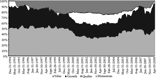
Figure 11 Factor Weights of the Trading Strategy

We determine the allocation to specific factors by solving the following optimization problem:

with the budget constraint

where is the covariance matrix of factor returns, Value and Growth are the sets of value and growth factors, and δi is equal to one if wi > 0 or zero otherwise.

We constrain the minimum exposure to values factors to be greater than or equal to 35% of the weight in the model based on the belief that there is a systematic long-term premium to value.

Using the returns of our factors, we perform this optimization monthly to determine which factors to hold and in what proportions. Figure 11 displays how the factor weights change over time.

In the next step, we use the factor weights to determine the attractiveness of the stocks in our universe. We score each stock in the universe by multiplying the standardized values of the factors by the weights provided by the optimization of our factors. Stocks with high scores are deemed attractive and stocks with low scores are deemed unattractive.

To evaluate how the model performs, we sort the scores of stocks into five equally weighted portfolios and evaluate the returns of these portfolios. Table 1(A) provides summary statistics of the returns for each portfolio. Note that there is a monotonic increasing relationship among the portfolios with portfolio 1 (q1) earning the highest return and portfolio 5 (q5) earning the lowest return. Over the entire period, the long-short portfolio (LS) that is long portfolio 1 and short portfolio 5 averages about 1% per month with a monthly Sharpe ratio of 0.33. Its return is statistically significant at the 97.5% level.

Table 1 Summary of Model Results
A. Summary Statistics of the Model Returns

Figure 12 Cumulative Return of the Model

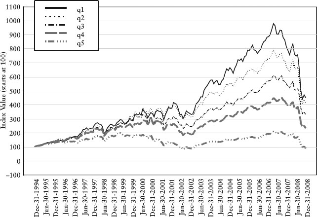
Table 1(B) shows the monthly average stock turnover of portfolio 1 (q1) and portfolio 5 (q5). Understanding how turnover varies from month to month for a trading strategy is important. If turnover is too high then it might be prohibitive to implement because of execution costs. While beyond the scope of this entry, we could explicitly incorporate transaction costs in this trading strategy using a market impact model.22 Due to the dynamic nature of our trading strategy—where active factors may change from month to month—our turnover of 20% is a bit higher than what would be expected using a static approach.

We evaluate the monthly information coefficient between the model scores and subsequent return. This analysis provides information on how well the model forecasts return. The monthly mean information coefficient of the model score is 0.03 and is statistically significant at the 99% level. The monthly standard deviation is 0.08. We note that both the information coefficients and returns were stronger and more consistent in the earlier periods.

Figure 12 displays the cumulative return to portfolio 1 through portfolio 5. Throughout the entire period there is a monotonic relationship between the portfolios. To evaluate the overall performance of the model, we analyze the performance of the long-short portfolio returns. We observe that the model performs well in December 1994 to May 2007 and April 2008 to June 2008. This is due to the fact that our model correctly picked the factors that performed well in those periods. We note that the model performs poorly in the period July 2007–April 2008, losing an average of 1.09% a month. The model appears to suffer from the same problems many quantitative equity funds and hedge funds faced during this period.23 The worst performance in a single month was –6.87, occurring in January 2001, and the maximum drawdown of the model was −13.7%, occurring during the period from May 2006 (peak) to June 2008 (trough).24

To more completely understand the return and risk characteristic of the strategy, we would have to perform a more detailed analysis, including risk and performance attribution, and model sensitivity analysis over the full period as well as over subperiods. As the turnover is on the higher side, we may also want to introduce turnover constraints or use a market impact model.

Periods of poor performance of a strategy should be disconcerting to any analyst. The poor performance of the model during the period June 2007–March 2008 indicates that many of the factors we use were not working. We need to go back to each individual factor and analyze them in isolation over this time frame. In addition, this highlights the importance of research to improve existing factors and develop new ones using unique data sources.

BACKTESTING

In the research phase of the trading strategy, model scores are converted into portfolios and then examined to assess how these portfolios perform over time. This process is referred to as backtesting a strategy. The backtest should mirror as closely as possible the actual investing environment incorporating both the investment’s objectives and the trading environment.

When it comes to mimicking the trading environment in backtests, special attention needs to be given to transaction costs and liquidity considerations. The inclusion of transaction costs is important because they may have a major impact on the total return. Realistic market impact and trading costs estimates affect what securities are chosen during portfolio construction. Liquidity is another attribute that needs to be evaluated. The investable universe of stocks should be limited to stocks where there is enough liquidity to be able to get in and out of positions.

Portfolio managers may use a number of constraints during portfolio construction. Frequently these constraints are derived from the portfolio policy of the firm, risk management policy, or investor objectives. Common constraints include upper and lower bounds for each stock, industry, or risk factor—as well as holding size limits, trading size limits, turnover, and the number of assets long or short.

To ensure the portfolio construction process is robust we use sensitivity analysis to evaluate our results. In sensitivity analysis we vary the different input parameters and study their impact on the output parameters. If small changes in inputs give rise to large changes in outputs, our process may not be robust enough. For example, we may eliminate the five best and worst performing stocks from the model, rerun the optimization, and evaluate the performance. The results should be similar as the success of a trading strategy should not depend on a handful of stocks.

We may want to determine the effect of small changes in one or more parameters used in the optimization. The performance of the optimal portfolio should in general not differ significantly after we have made these small changes.

Another useful test is to evaluate a model by varying the investment objective. For example, we may evaluate a model by building a low-tracking-error portfolio, a high-tracking-error portfolio, and a market-neutral portfolio. If the returns from each of these portfolios are decent, the underlying trading strategy is more likely to be robust.

Understanding In-Sample and Out-of-Sample Methodologies

There are two basic backtesting methodologies: in-sample and out-of-sample. It is important is to understand the nuances of each.

We refer to a backtesting methodology as an in-sample methodology when the researcher uses the same data sample to specify, calibrate, and evaluate a model.

An out-of-sample methodology is a backtesting methodology where the researcher uses a subset of the sample to specify and calibrate a model, and then evaluates the forecasting ability of the model on a different subset of data. There are two approaches for implementing an out-of-sample methodology. One approach is the split-sample method. This method splits the data into two subsets of data where one subset is used to build the model while the remaining subset is used to evaluate the model.

A second method is the recursive out-of-sample test. This approach uses a sequence of recursive or rolling windows of past history to forecast a future value and then evaluates that value against the realized value. For example, in a rolling regression–based model we will use data up to time t to calculate the coefficients in the regression model. The regression model forecasts the t + h dependent values, where h > 0. The prediction error is the difference between the realized value at t + h and the predicted value from the regression model. At t + 1 we recalculate the regression model and evaluate the predicted value of t + 1 + h against realized value. We continue this process throughout the sample.

The conventional thinking among econometricians is that in-sample tests tend to reject the null hypotheses of no predictability more often than out-of-sample tests. This view is supported by many researchers because they reason that in-sample tests are unreliable, often finding spurious predictability. Two reasons given to support this view are the presence of unmodeled structural changes in the data and the use of techniques that result in data mining and model overfitting.

Inoune and Kilian (2002) question this conventional thinking. They use asymptotic theory to evaluate the “trade-offs between in-sample tests and out-of-sample tests of predictability in terms of their size and power.” They argue strong in-sample results and weak out-of-sample results are not necessarily evidence that in-sample tests are not reliable. Out-of-sample tests using sample-splitting result in a loss of information and lower power for small samples. As a result, an out-of-sample test may fail to detect predictability while the in-sample test will correctly identify predictability. They also show that out-of-sample tests are not more robust to parameter instability that results from unmodeled structural changes.

A Comment on the Interaction between Factor-Based Strategies and Risk Models

Frequently, different factor models are used to calculate the risk inputs and the expected return forecasts in a portfolio optimization. A common concern is the interaction between factors in the models for risk and expected returns. Lee and Stefek (2008) evaluate the consequences of using different factor models, and conclude that (1) using different models for risk and alpha can lead to unintended portfolio exposures that may worsen performance; (2) aligning risk factors with alpha factors may improve information ratios; and (3) modifying the risk model by including some of the alpha factors may mitigate the problem.

Table 2 Total Return Report (annualized)

BACKTESTING OUR FACTOR TRADING STRATEGY

Using the model scores from the trading strategy example, we build two optimized portfolios and evaluate their performance. Unlike the five equally weighted portfolios built only from model scores, the models we now discuss were built to mirror as close as possible tradable portfolios a portfolio manager would build in real time. Our investable universe is the Russell 1000. We assign alphas for all stock in the Russell 1000 with our dynamic factor model. The portfolios are long only and benchmarked to the S&P 500. The difference between the portfolios is in their benchmark tracking error. For the low-tracking error portfolio the risk aversion in the optimizer is set to a high value, sectors are constrained to plus or minus 10% of the sector weightings in the benchmark, and portfolio beta is constrained to 1.00. For the high-tracking error portfolio, the risk aversion is set to a low value, the sectors are constrained to plus or minus 25% of the sector weightings in the benchmark, and portfolio beta is constrained to 1.00. Rebalancing is performed once a month. Monthly turnover is limited to 10% of the portfolio value for the low-tracking error portfolio and 15% of the portfolio value for the high-tracking error portfolio.

Table 2 presents the results of our backtest. The performance numbers are gross of fees and transaction costs. Performance over the entire period is good and consistent throughout. The portfolios outperform the benchmark over the various time periods. The resulting annualized Sharpe ratios over the full period are 0.66 for the low-tracking error portfolio, 0.72 for the high-tracking error portfolio, and 0.45 for the S&P 500.25

KEY POINTS

• The four most commonly used approaches for the evaluation of return premiums and risk characteristics to factors are portfolio sorts, factor models, factor portfolios, and information coefficients.
• The portfolio sorts approach ranks stocks by a particular factor into a number of portfolios. The sorting methodology should be consistent with the characteristics of the distribution of the factor and the economic motivation underlying its premium.
• The information ratio (IR) is a statistic for summarizing the risk-adjusted performance of an investment strategy and is defined as the ratio of average excess return to the standard deviation of return.
• We distinguish between contemporaneous and forecasting factor models, dependent on whether both left- and right-hand side variables (returns and factors) have the same time subscript, or the time subscript of the left-hand side variable is greater.
• The three most common violations of classical regression theory that occur in cross-sectional factor models are (1) the errors in variables problem, (2) common variation in residuals such as heteroskedasticity and serial correlation, and (3) multicollinearity. There are statistical techniques that address the first two. The third issue is best dealt with by removing collinear variables from the regression, or by increasing the sample size.
• The Fama-MacBeth regression addresses the inference problem caused by the correlation of the residuals in cross-sectional regressions.
• The information coefficient (IC) is used to evaluate the return forecast ability of a factor. It measures the cross-sectional correlation between a factor and its subsequent realized return.
• Factor portfolios are used to measure the information content of a factor. The objective is to mimic the return behavior of a factor and minimize the residual risk. We can build factor portfolios using a factor model or an optimization. An optimization is more flexible as it is able to incorporate constraints.
• Analyzing the performance of different factors is an important part of the development of a factor-based trading strategy. This process begins with understanding the time-series properties of each factor in isolation and then studying how they interact with each other.
• Techniques used to combine and weight factors to build a trading strategy model include the data driven, the factor model, the heuristic, and the optimization approaches.
• An out-of-sample methodology is a backtesting methodology where the researcher uses a subset of the sample to specify a model and then evaluates the forecasting ability of the model on a different subset of data. There are two approaches for implementing an out-of-sample methodology: the split-sample approach and the recursive out-of-sample test.
• Caution should be exercised if different factor models are used to calculate the risk inputs and the expected return forecasts in a portfolio optimization.

APPENDIX: THE COMPUSTAT POINT-IN-TIME, IBES CONSENSUS DATABASES AND FACTOR DEFINITIONS

The factors used in this entry were constructed on a monthly basis with data from the Compustat Point-In-Time and IBES Consensus databases. Our sample includes the largest 1,000 stocks by market capitalization over the period December 31, 1989, to December 31, 2008.

The Compustat Point-In-Time database (Capital IQ, Compustat, http://www.compustat.com) contains quarterly financial data from the income, balance sheet, and cash flow statements for active and inactive companies. This database provides a consistent view of historical financial data, both reported data and subsequent restatements, the way it appeared at the end of any month. Using these data allows the researcher to avoid common data issues such as survivorship and look-ahead bias. The data are available from March 1987.

The Institutional Brokers Estimate System (IBES) database (Thomson Reuters, http://www.thomsonreuters.com) provides actual earnings from companies and estimates of various financial measures from sell-side analysts. The estimated financial measures include estimates of earnings, revenue and sales, operating profit, analyst recommendations, and other measures. The data are offered on a summary (consensus) level or detailed (analyst-by-analyst) basis. The U.S. data cover reported earnings estimates and results since January 1976.

The factors used in this entry are defined as follows. (LTM refers to the last four reported quarters.)

Value Factors

Operating income before depreciation to enterprise value = EBITDA/EV

where

and

Quality Factors

where

and

where

and

Growth

Momentum

Summary Statistics

The following table contains monthly summary statistics of the factors defined previously. Factor values greater than the 97.5 percentile or less than the 2.5 percentile are considered outliers.

We set factor values greater than the 97.5 percentile value to the 97.5 percentile value, and factor values less than the 2.5 percentile value to the 2.5 percentile value, respectively.

NOTES

1. For a good overview of the most common issues, see Berk (2000) and references therein.

2. Grinold and Kahn (1999) discuss the differences between the t-statistic and the information ratio. Both measures are closely related in their calculation. The t-statistic is the ratio of mean return of a strategy to its standard error. Grinold and Kahn state the related calculations should not obscure the distinction between the two ratios. The t-statistic measures the statistical significance of returns while the IR measures the risk-reward trade-off and the value added by an investment strategy.

3. See, for example, Fama and French (2004).

4. One approach is to use the Bayesian or model averaging techniques. For more details on the Bayesian approach, see, for example, Rachev, Hsu, Bagasheva, and Fabozzi (2008).

5. For a discussion of dealing with these econometric problems, see Chapter 2 in Fabozzi, Focardi, and Kolm (2010).

6. We cover Fama-MacBeth regression in this section.

7. Fama and French (2004).

8. See, for example, Grinold and Kahn (1999) and Qian, Hua, and Sorensen (2007).

9. A factor normalized z-score is given by the formula z-score = (f − )/std(f) where f is the factor, is the mean, and std(f) is the standard deviation of the factor.

10. We are conforming to the notation used in Qian and Hua (2004). To avoid confusion, Qian and Hua use dis() to describe the cross-sectional standard deviation and std() to describe the time series standard deviation.

11. The earnings estimates come from the IBES database. See the appendix for a more detailed description of the data.

12. This derivation of factor portfolios is presented in Grinold and Kahn (1999).

13. See Melas, Suryanarayanan, and Cavaglia (2009).

14. An exception is the constraint on the number of assets that results in integer constraints.

15. For a more detailed discussion on portfolio optimization problems and optimization software see, for example, Fabozzi, Kolm, Pachamanova, and Focardi (2007).

16. The hit rate is calculated as

where yit is one-step ahead realized value and is the one-step ahead predicted value.

17. For calculation of this measure, see Diebold and Mariano (2005).

18. The nine factors are return on assets, change in return on assets, cash flow from operations scaled by total assets, cash compared to net income scaled by total assets, change in long-term debt/assets, change in current ratio, change in shares outstanding, change in gross margin, and change in asset turnover.

19. Zlotnikov, Larson, Cheung, Kalaycioglu, Lao, and Apoian (2007).

20. Zlotnikov, Larson, Wally, Kalaycioglu, Lao, and Apoian (2007).

21. We use a combination of growth, value, quality, and momentum factors. The appendix to this entry contains definitions of all of them.

22. Cerniglia and Kolm (2010).

23. See Rothman (2007) and Daniel (2007).

24. We ran additional analysis on the model by extending the holding period of the model from 1 to 3 months. The results were much stronger as returns increased to 1.6% per month for a two-month holding period and 1.9% per month for a three-month holding period. The risk as measured by drawdown was higher at –17.4% for a two-month holding period and –29.5% for the three-month holding period.

25. Here we calculate the Sharpe ratio as portfolio excess return (over the risk-free rate) divided by the standard deviation of the portfolio excess return.

REFERENCES

Andrews, D. W. K. (1991). Heteroskedasticity and autocorrelation consistent covariance matrix estimation. Econometrica 59, 3: 817–858.

Berk, J. B. (2000). Sorting out sorts. Journal of Finance 55, 1: 407–427.

Cerniglia, J. A., and Kolm, P. N. (2010). Factor-based trading strategies and market impact costs. Working paper, Courant Institute of Mathematical Sciences, New York University.

Cochrane, J. H. (2005). Asset Pricing. Princeton, NJ: Princeton University Press.

Daniel, K. (2001). The liquidity crunch in quant equities: Analysis and implications. Goldman Sachs Asset Management, December 13, 2007, presentation from The Second New York Fed–Princeton Liquidity Conference.

Deistler, M., and Hamann, E. (2005). Identification of factor models for forecasting returns. Journal of Financial Econometrics 3, 2: 256–281.

Diebold, F. X., and Mariano, R. S. (2005). Comparing predictive accuracy. Journal of Business and Economic Statistics 13, 3: 253–263.

Fabozzi, F. J., Focardi, S. M., and Kolm, P. N. (2010). Quantitative Equity Investing. Hoboken, NJ: John Wiley & Sons.

Fabozzi, F. J., Kolm, P. N., Pachamanova, D., and Focardi, S. M. (2007). Robust Portfolio Optimization and Management. Hoboken, NJ: John Wiley & Sons.

Fama, E. F., and French, K. R. (2004). The capital asset pricing model: Theory and evidence. Journal of Economic Perspectives 18, 3: 25–46.

Fama, E. F., and MacBeth, J. D. (1973). Risk, return, and equilibrium: Empirical tests. Journal of Political Economy 81, 3: 607–636.

Gow, I. D., Ormazabal, G., and Taylor, D. J. (2009). Correcting for cross-sectional and time-series dependence in accounting research. Working paper, Kellogg School of Business and Stanford Graduate School.

Grinold, R. C., and Kahn, R. N. (1999). Active Portfolio Management: A Quantitative Approach for Providing Superior Returns and Controlling Risk. New York: McGraw-Hill.

Inoune, A., and Kilian, L. (2002). In-sample or out-of-sample tests of predictability: Which one should we use? Working paper, North Carolina State University and University of Michigan.

Hua, R., and Qian, E. (2004). Active risk and information ratio. Journal of Investment Management 2, 3: 1–15.

Kolm, P. N. (2010). Multi-period portfolio optimization with transaction costs, alpha decay, and constraints. Working paper, Courant Institute of Mathematical Sciences, New York University.

Lee, J-H., and Stefek, D. (2008). Do risk factors eat alphas? Journal of Portfolio Management 34, 4: 12–24.

Melas, D., Suryanarayanan, R., and Cavaglia, S. (2009). Efficient replication of factor returns. MSCI Barra Research Insight, June.

Newey, W. K., and West, K. D. (1987). A simple, positive semidefinite heteroskedasticity and autocorrelation consistent covariance matrix. Econometrica 56, 3: 703–708.

Patton, A. J., and Timmermann, A. (2009). Monotonicity in asset returns: New tests with applications to the term structure, the CAPM and portfolio sorts. Working paper, University of California–San Diego.

Petersen, M. A. (2009). Estimating standard errors in finance panel sets: Comparing approaches. Review of Financial Studies 22, 1: 435–480.

Piotroski, J. D. (2000). Value investing: The use of historical financial statement information to separate winners from losers. Journal of Accounting Research 38 (3 supplement): 1–41.

Qian, E. E., Hua, R. H., and Sorensen, E. H. (2007). Quantitative Portfolio Management: Modern Techniques and Applications. New York: Chapman & Hall/CRC.

Rachev, S. T., Hsu, J. S. J., Bagasheva, B. S., and Fabozzi, F. J. (2008). Bayesian Methods in Finance. Hoboken, NJ: John Wiley & Sons.

Rothman, M. S. (2007). Turbulent times in quant land. Lehman Brothers Equity Research, August 9.

Sneddon, L. (2008). The tortoise and the hare: Portfolio dynamics for active managers. Journal of Investing 17, 4: 106–111.

Sorensen, E. H., Hua, R., and Qian, E. (2005). Contextual fundamentals, models, and active management. Journal of Portfolio Management 32, 1: 23–36.

Sorensen, E. H., Hua, R., Qian, E., and Schoen, R. (2004). Multiple alpha sources and active management. Journal of Portfolio Management 30, 2: 39–45.

West, K. D. (2006). Forecast evaluation. In G. Elliot, C. W. J. Granger, and A. G. Timmermann (Eds.), Handbook of Economic Forecasting, Vol.1. Amsterdam: Elsevier.

Zlotnikov, V., Larson, A. M., Cheung, W., Kalaycioglu, S., Lao, R. D., and Apoian, Z. A. (2007). Quantitative research: Survey of quantitative models—Vastly different rankings and performance, despite similarity in factor exposures. Quantitative Research, Bernstein Research, January 16.

Zlotnikov, V., Larson, A. M., Kalaycioglu, S., Lao, R. D., and Apoian, Z. A. (2007). Quantitative research: Survey of quantitative models—Continued emphasis on EV/EBIT, momentum, increased focus on capital use; some evidence on non-linear factor implementation; low return consistency. Quantitative Research, Bernstein Research, November 21.