
Factor-Based Equity Portfolio Construction and Analysis
Common stock investment strategies can be broadly classified into the following categories: (1) factor-based trading strategies (also called stock selectiont or alpha models), (2) statistical arbitrage, (3) high-frequency strategies, and (4) event studies. Factors and factor-based models form the core of a major part of today’s quantitative trading strategies. The focus of this entry is on developing trading strategies based on factors constructed from common (cross-sectional) characteristics of stocks. For this purpose, first we provide a definition of factors. We then examine the major sources of risk associated with trading strategies, and demonstrate how factors are constructed from company characteristics and market data. The quality of the data used in this process is critical. We examine several data cleaning and adjustment techniques to account for problems occurring with backfilling and restatements of data, missing data, inconsistently reported data, as well as survivorship and look-ahead biases. In the last section of this entry, we discuss the analysis of the statistical properties of factors.
Table 1 Summary of Well-Known Factors and Their Underlying Economic Rationale
| Factor | Economic Rationale |
| Dividend yield | Investors prefer to immediately receive receipt of their investment returns. |
| Value | Investors prefer stocks with low valuations. |
| Size (market capitalization) | Smaller companies tend to outperform larger companies. |
| Asset turnover | This measure evaluates the productivity of assets employed by a firm. Investors believe higher turnover correlates with higher future return. |
| Earnings revisions | Positive analysts’ revisions indicate stronger business prospects and earnings for a firm. |
| Growth of fiscal year 1 and fiscal year 2 earnings estimates | Investors are attracted to companies with growing earnings. |
| Momentum | Investors prefer stocks that have had good past performance. |
| Return reversal | Investors overreact to information, that is, stocks with the highest returns in the current month tend to earn lower returns the following month. |
| Idiosyncratic risk | Stocks with high idiosyncratic risk in the current month tend to have lower returns the following month. |
| Earnings surprises | Investors like positive earnings surprises and dislike negative earnings surprises. |
| Accounting accruals | Companies with earnings that have a large cash component tend to have higher future returns. |
| Corporate governance | Firms with better corporate governance tend to have higher firm value, higher profits, higher sales growth, lower capital expenditures, and fewer corporate acquisitions. |
| Executive compensation factors | Firms that align compensation with shareholders’ interest tend to outperform. |
| Accounting risk factors | Companies with lower accounting risk tend to have higher future returns. |
In a series of examples, we show the individual steps for developing a basic trading strategy. The purpose of these examples is not to provide yet another profitable trading strategy, but rather to illustrate the process an analyst may follow when performing research. In fact, the factors that we use for this purpose are well known and have for years been exploited by industry practitioners. The value added of these examples is in the concrete illustration of the research and development process of a factor-based trading model.
FACTOR-BASED TRADING
Since the first version of the classic text on security analysis by Benjamin Graham and David Dodd1—considered to be the Bible on the fundamental approach to security analysis—was first published in 1934, equity portfolio management and trading strategies have developed considerably. Graham and Dodd were early contributors to factor-based strategies because they extended traditional valuation approaches by using information throughout the financial statements2 and by presenting concrete rules of thumb to be used to determine the attractiveness of securities.3
Today’s quantitative managers use factors as fundamental building blocks for trading strategies. Within a trading strategy, factors determine when to buy and sell securities. We define a factor as a common characteristic among a group of assets. In the equities market, it could be a particular financial ratio such as the price–earnings (P/E) or the book–price (B/P) ratios. Some of the most well-known factors and their underlying basic economic rationale references are provided in Table 1.
Most often this basic definition is expanded to include additional objectives. First, factors frequently are intended to capture some economic intuition. For instance, a factor may help understand the prices of assets by reference to their exposure to sources of macroeconomic risk, fundamental characteristics, or basic market behavior. Second, we should recognize that assets with similar factors (characteristics) tend to behave in similar ways. This attribute is critical to the success of a factor. Third, we would like our factor to be able to differentiate across different markets and samples. Fourth, we want our factor to be robust across different time periods.
Factors fall into three categories— macroeconomic influences, cross-sectional characteristics, and statistical factors. Macro-economic influences are time series that measure observable economic activity. Examples include interest rate levels, gross domestic production, and industrial production. Cross-sectional characteristics are observable asset specifics or firm characteristics. Examples include dividend yield, book value, and volatility. Statistical factors are unobservable or latent factors common across a group of assets. These factors make no explicit assumptions about the asset characteristics that drive commonality in returns. Statistical factors are not derived using exogenous data but are extracted from other variables such as returns. These factors are calculated using various statistical techniques such as principal components analysis or factor analysis.
Within asset management firms, factors and forecasting models are used for a number of purposes. Those purposes could be central to managing portfolios. For example, a portfolio manager can directly send the model output to the trading desk to be executed. In other uses, models provide analytical support to analysts and portfolio management teams. For instance, models are used as a way to reduce the investable universe to a manageable number of securities so that a team of analysts can perform fundamental analysis on a smaller group of securities.
Factors are employed in other areas of financial theory, such as asset pricing, risk management, and performance attribution. In asset pricing, researchers use factors as proxies for common, undiversifiable sources of risk in the economy to understand the prices or values of securities to uncertain payments. Examples include the dividend yield of the market or the yield spread between a long-term bond yield and a short-term bond yield.4 In risk management, risk managers use factors in risk models to explain and to decompose variability of returns from securities, while portfolio managers rely on risk models for covariance construction, portfolio construction, and risk measurement. In performance attribution, portfolio managers explain past portfolio returns based on the portfolio’s exposure to various factors. Within these areas, the role of factors continues to expand. Recent research presents a methodology for attributing active return, tracking error, and the information ratio to a set of custom factors.5
The focus in this entry is on using factors to build equity forecasting models, also referred to as alpha or stock selection models. The models serve as mathematical representations of trading strategies. The mathematical representation uses future returns as dependent variables and factors as independent variables.
DEVELOPING FACTOR-BASED TRADING STRATEGIES
The development of a trading strategy has many similarities with an engineering project. We begin by designing a framework that is flexible enough so that the components can be easily modified, yet structured enough that we remain focused on our end goal of designing a profitable trading strategy.
Basic Framework and Building Blocks
The typical steps in the development of a trading strategy are:
- Defining a trading idea or investment strategy.
- Developing factors.
- Acquiring and processing data.
- Analyzing the factors.
- Building the strategy.
- Evaluating the strategy.
- Backtesting the strategy.
- Implementing the strategy.
In what follows, we take a closer look at each step.
Defining a Trading Idea or Investment Strategy
A successful trading strategy often starts as an idea based on sound economic intuition, market insight, or the discovery of an anomaly. Background research can be helpful in order to understand what others have tried or implemented in the past.
We distinguish between a trading idea and trading strategy based on the underlying economic motivation. A trading idea has a more short-term horizon often associated with an event or mispricing. A trading strategy has a longer horizon and is frequently based on the exploitation of a premium associated with an anomaly or a characteristic.
Developing Factors
Factors provide building blocks of the model used to build an investment strategy. We introduced a general definition of factors earlier in this entry. After having established the trading strategy, we move from the economic concepts to the construction of factors that may be able to capture our intuition. In this entry, we provide a number of examples of factors based on the cross-sectional characteristics of stocks.
Acquiring and Processing Data
A trading strategy relies on accurate and clean data to build factors. There are a number of third-party solutions and databases available for this purpose such as Thomson MarketQA,6 Factset Research Systems,7 and Compustat Xpressfeed.8
Analyzing the Factors
A variety of statistical and econometric techniques must be performed on the data to evaluate the empirical properties of factors. This empirical research is used to understand the risk and return potential of a factor. The analysis is the starting point for building a model of a trading strategy.
Building the Strategy
The model represents a mathematical specification of the trading strategy. There are two important considerations in this specification: the selection of which factors and how these factors are combined. Both considerations need to be motivated by the economic intuition behind the trading strategy. We advise against model specification being strictly data driven because that approach often results in overfitting the model and consequently overestimating forecasting quality of the model.
Evaluating, Backtesting, and Implementing the Strategy
The final step involves assessing the estimation, specification, and forecast quality of the model. This analysis includes examining the goodness of fit (often done in sample), forecasting ability (often done out of sample), and sensitivity and risk characteristics of the model.
RISK TO TRADING STRATEGIES
In investment management, risk is a primary concern. The majority of trading strategies are not risk free but rather subject to various risks. It is important to be familiar with the most common risks in trading strategies. By understanding the risks in advance, we can structure our empirical research to identify how risks will affect our strategies. Also, we can develop techniques to avoid these risks in the model construction stage when building the strategy.
We describe the various risks that are common to factor trading strategies as well as other trading strategies such as risk arbitrage. Many of these risks have been categorized in the behavioral finance literature.9 The risks discussed include fundamental risk, noise trader risk, horizon risk, model risk, implementation risk, and liquidity risk.
Fundamental risk is the risk of suffering adverse fundamental news. For example, say our trading strategy focuses on purchasing stocks with high earnings-to-price ratios. Suppose that the model shows a pharmaceutical stock maintains a high score. After purchasing the stock, the company releases a news report that states it faces class-action litigation because one of its drugs has undocumented adverse side effects. While during this period other stocks with high earnings-to-price ratio may perform well, this particular pharmaceutical stock will perform poorly despite its attractive characteristic. We can minimize the exposure to fundamental risk within a trading strategy by diversifying across many companies. Fundamental risk may not always be company specific; sometimes this risk can be systemic. Some examples include the exogenous market shocks of the stock market crash in 1987, the Asian financial crisis in 1997, and the tech bubble in 2000. In these cases, diversification was not that helpful. Instead, portfolio managers that were sector or market neutral in general fared better.
Noise trader risk is the risk that a mispricing may worsen in the short run. The typical example includes companies that clearly are undervalued (and should therefore trade at a higher price). However, because noise traders may trade in the opposite direction, this mispricing can persist for a long time. Closely related to noise trader risk is horizon risk. The idea here is that the premium or value takes too long to be realized, resulting in a realized return lower than a target rate of return.
Model risk, also referred to as misspecification risk, refers to the risk associated with making wrong modeling assumptions and decisions. This includes the choice of variables, methodology, and context the model operates in. There are different sources that may result in model misspecification and there are several remedies based on information theory, Bayesian methods, shrinkage, and random coefficient models.10
Implementation risk is another risk faced by investors implementing trading strategies. This risk category includes transaction costs and funding risk. Transaction costs such as commissions, bid-ask spreads, and market impact can adversely affect the results from a trading strategy. If the strategy involves shorting, other implementation costs arise such as the ability to locate securities to short and the costs to borrow the securities. Funding risk occurs when the portfolio manager is no longer able to get the funding necessary to implement a trading strategy. For example, many statistical arbitrage funds use leverage to increase the returns of their funds. If the amount of leverage is constrained, then the strategy will not earn attractive returns. Khandani and Lo (2007) confirm this example by showing that greater competition and reduced profitability of quantitative strategies today require more leverage to maintain the same level of expected return.
Liquidity risk is a concern for investors. Liquidity is defined as the ability to (1) trade quickly without significant price changes, and (2) trade large volumes without significant price changes. Cerniglia and Kolm (2009) discuss the effects of liquidity risk during the “quant crisis” in August 2007. They show how the rapid liquidation of quantitative funds affected the trading characteristics and price impact of trading individual securities as well as various factor-based trading strategies.
These risks can detract or contribute to the success of a trading strategy. It is obvious how these risks can detract from a strategy. What is not always clear is when any one of these unintentional risks contributes to a strategy. That is, sometimes when we build a trading strategy we take on a bias that is not obvious. If there is a premium associated with this unintended risk, then a strategy will earn additional return. Later the premium to this unintended risk may disappear. For example, a trading strategy that focuses on price momentum performed strongly in the calendar years of 1998 and 1999. What an investor might not notice is that during this period the portfolio became increasingly weighted toward technology stocks, particularly Internet-related stocks. During 2000, these stocks severely underperformed.
DESIRABLE PROPERTIES OF FACTORS
Factors should be founded on sound economic intuition, market insight, or an anomaly. In addition to the underlying economic reasoning, factors should have other properties that make them effective for forecasting.
It is an advantage if factors are intuitive to investors. Many investors will only invest in a particular fund if they understand and agree with the basic ideas behind the trading strategies. Factors give portfolio managers a tool in communicating to investors what themes they are investing in.
The search for the economic meaningful factors should avoid strictly relying on pure historical analysis. Factors used in a model should not emerge from a sequential process of evaluating successful factors while removing less favorable ones.
Most importantly, a group of factors should be parsimonious in its description of the trading strategy. This requires careful evaluation of the interaction between the different factors. For example, highly correlated factors will cause the inferences made in a multivariate approach to be less reliable. Another possible problem when using multiple factors is the possibility of overfitting in the modeling process.
Any data set contains outliers, that is, observations that deviate from the average properties of the data. Outliers are not always trivial to handle and sometimes we may want to exclude them and other times not. For example, they could be erroneously reported or legitimate abnormal values. Later in this entry we discuss a few standard techniques to perform data cleaning. The success or failure of factors selected should not depend on a few outliers. In most cases, it is desirable to construct factors that are reasonably robust to outliers.
SOURCES FOR FACTORS
How do we find factors? The sources are widespread with no one source clearly dominating. Employing a variety of sources seems to provide the best opportunity to uncover factors that will be valuable for developing a new model.
There are a number of ways to develop factors based on economic foundations. It may start with thoughtful observation or study of how market participants act. For example, we may ask ourselves how other market participants will evaluate the prospects of the earnings or business of a firm. We may also want to consider what stock characteristics investors will reward in the future. Another common approach is to look for inefficiencies in the way that investors process information. For instance, research may discover that consensus expectations of earnings estimates are biased.
A good source for factors is the various reports released by the management of companies. Many reports contain valuable information and may provide additional context on how management interprets the company results and financial characteristics. For example, quarterly earning reports (10-Qs) may highlight particular financial metrics relevant to the company and the competitive space they are operating within. Other company financial statements and SEC filings, such as the 10-K or 8-K, also provide a source of information to develop factors. It is often useful to look at the financial measures that management emphasize in their comments.
Factors can be found through discussions with market participants such as portfolio managers and traders. Factors are uncovered by understanding the heuristics experienced investors have used successfully. These heuristics can be translated into factors and models.
Wall Street analyst reports—also called sell-side reports or equity research reports—may contain valuable information. The reader is often not interested in the final conclusions, but rather in the methodology or metrics the analysts use to forecast the future performance of a company. It may also be useful to study the large quantity of books written by portfolio managers and traders that describe the process they use in stock selection.
Academic literature in finance, accounting, and economics provides evidence of numerous factors and trading strategies that earn abnormal returns. Not all strategies will earn abnormal profits when implemented by practitioners, for example, because of institutional constraints and transaction costs. Bushee and Raedy (2006) find that trading strategy returns are significantly decreased due to issues such as price pressure, restrictions against short sales, incentives to maintain an adequately diversified portfolio, and restrictions to hold no more than 5% ownership in a firm.
In uncovering factors, we should put economic intuition first and data analysis second. This avoids performing pure data mining or simply overfitting our models to past history. Research and innovation is the key to finding new factors. Today, analyzing and testing new factors and improving upon existing ones is itself a big industry.
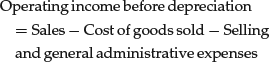
BUILDING FACTORS FROM COMPANY CHARACTERISTICS
The following sections focus on the techniques for building factors from company characteristics. Often we desire our factors to relate the financial data provided by a company to metrics that investors use when making decisions about the attractiveness of a stock such as valuation ratios, operating efficiency ratios, profitability ratios, and solvency ratios. Factors should also relate to the market data such as analysts’ forecasts, prices and returns, and trading volume.
WORKING WITH DATA
In this section, we discuss how to work with data and data quality issues, including some well-probed techniques used to improve the quality of the data. Though the role of getting and analyzing data can be mundane and tedious, we need not forget that high-quality data are critical to the success of a trading strategy. It is important to realize model output is only as good as the data used to calibrate it. As the saying goes: “Garbage in, garbage out.”
Understanding the structure of financial data is important. We distinguish three different categories of financial data: time series, cross-sectional, and panel data. Time series data consist of information and variables collected over multiple time periods. Cross-sectional data consist of data collected at one point in time for many different companies (the cross-section of companies of interest). A panel data set consists of cross-sectional data collected at different points in time. We note that a panel data set may not be homogeneous. For instance, the cross-section of companies may change from one point in time to another.
Data Integrity
Quality data maintain several attributes such as providing a consistent view of history, maintaining good data availability, containing no survivorship, and avoiding look-ahead bias. As all data sets have their limitations, it is important for the quantitative researcher to be able to recognize the limitations and adjust the data accordingly.
Data used in research should provide a consistent view of history. Two common problems that distort the consistency of financial data are backfilling and restatements of data. Backfilling of data happens when a company is first entered into a database at the current period and its historical data are also added. This process of backfilling data creates a selection bias because we now find historical data on this recently added company when previously it was not available. Restatements of data are prevalent in distorting consistency of data. For example, if a company revises its earnings per share numbers after the initial earnings release, then many database companies will overwrite the number originally recorded in the database with the newly released figure.
A frequent and common concern with financial databases is data availability. First, data items may only be available for a short period of time. For example, there were many years when stock options were granted to employees but the expense associated with the option grant was not required to be disclosed in financial statements. It was not until 2005 that accounting standards required companies to recognize directly stock options as an expense on the income statement. Second, data items may be available for only a subset of the cross-section of firms. Some firms, depending on the business they operate in, have research and development expenses while others do not. For example, many pharmaceutical companies have research and development expenses while utilities companies do not. A third issue is that a data item may simply not be available because it was not recorded at certain points in time. Sometimes this happens for just a few observations, other times it is the case for the whole time-series for a specific data item for a company. Fourth, different data items are sometimes combined. For example, sometimes depreciation and amortization expenses are not a separate line item on an income statement. Instead it is included in cost of goods sold. Fifth, certain data items are only available at certain periodicities. For instance, some companies provide more detailed financial reports quarterly while others report more details annually. Sixth, data items may be inconsistently reported across different companies, sectors, or industries. This may happen as the financial data provider translates financial measures from company reports to the specific database items (incomplete mapping), thereby ignoring or not correctly making the right adjustments.
For these issues some databases provide specific codes to identify the causes of missing data. It is important to have procedures in place that can distinguish among the different reasons for the missing data and be able to make adjustments and corrections.
Two other common problems with databases are survivorship and look-ahead bias. Survivorship bias occurs when companies are removed from the database when they no longer exist. For example, companies can be removed because of a merger or bankruptcy. This bias skews the results because only successful firms are included in the entire sample. Look-ahead bias occurs when data are used in a study that would not have been available during the actual period analyzed. For example, the use of year-end earnings data immediately at the end of the reporting period is incorrect because the data are not released by the firm until several days or weeks after the end of the reporting period.
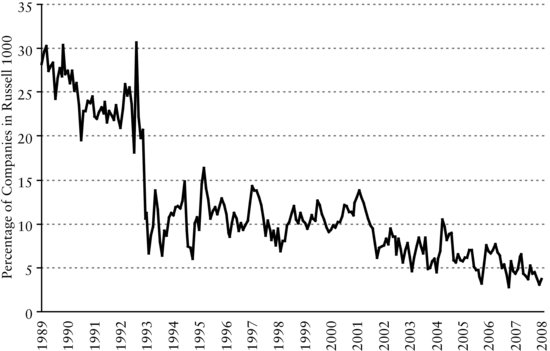
Figure 1 Percentage of Companies in Russell 1000 with Different Ranking According to the EBITDA/EV Factor
Data alignment is another concern when working with multiple databases. Many databases have different identifiers used to identify a firm. Some databases have vendor specific identifiers, others have common identifiers such as CUSIPs or ticker symbols. Unfortunately, CUSIPs and ticker symbols change over time and are often reused. This practice makes it difficult to link an individual security across multiple databases across time.
Example: The EBITDA/EV Factor
This example illustrates how the nuances of data handling can influence the results of a particular study. We use data from the Compustat Point-In-Time database and calculate the EBITDA/EV factor.11 This factor is defined as earnings before interest, taxes, depreciation, and amortization divided by enterprise value (EBITDA/EV). Our universe of stocks is the Russell 1000 from December 1989 to December 2008, excluding financial companies. We calculate EBITDA /EV by two equivalent but different approaches. Each approach differs by the data items used in calculating the numerator (EBITDA):
According to the Compustat manual, the following identity holds:
However, while this mathematical identity is true, this is not what we discover in the data. After we calculate the two factors, we form quintile portfolios of each factor and compare the individual holding rankings between the portfolio. Figure 1 displays the percentage differences in rankings for individual companies between the two portfolios. We observe that the results are not identical. As a matter of fact, there are large differences, particularly in the early period. In other words, the two mathematically equivalent approaches do not deliver the same empirical results.
Potential Biases from Data
There are numerous potential biases that may arise from data quality issues. It is important to recognize the direct effects of these data issues are not apparent a priori. We emphasize three important effects:12
Dealing with Common Data Issues
Most data sets are subject to some quality issues. To work effectively, we need to be familiar with data definitions and database design. We also need to use processes to reduce the potential impact of data problems as they could cause incorrect conclusions.
The first step is to become familiar with the data standardization process vendors use to collect and process data. For example, many vendors use different templates to store data. Specifically, the Compustat US database has one template for reporting income statement data, while the Worldscope Global database has four different templates depending on whether a firm is classified as a bank, insurance company, industrial company, or other financial company. Other questions related to standardization a user should be familiar with include:
- What are the sources of the data—publicly available financial statements, regulatory filings, newswire services, or other sources?
- Is there a uniform reporting template?
- What is the delay between publication of information and its availability in the database?
- Is the data adjusted for stock splits?
- Is history available for extinct or inactive companies?
- How is data handled for companies with multiple share classes?
- What is the process used to aggregate the data?
Understanding of the accounting principles underlying the data is critical. Here, two principles of importance are the valuation methodology and data disclosure or presentation. For the valuation, we should understand the type of cost basis used for the various accounting items. Specifically, are assets calculated using historical cost basis, fair value accounting, or another type? For accounting principles regarding disclosure and presentation, we need to know the definition of accounting terms, the format of the accounts, and the depth of detail provided.
Researchers creating factors that use financial statements should review the history of the underlying accounting principles. For example, the cash flow statement reported by companies has changed over the years. Effective for fiscal years ending July 15, 1988, Statement of Financial Accounting Standards No. 85 (SFAS No. 85) requires companies to report the Statement of Cash Flows. Prior to the adoption of that accounting standard, companies could report one of three statements: Working Capital Statement, Cash Statement by Source and Use of Funds, or Cash Statement by Activity. Historical analysis of any factor that uses cash flow items will require adjustments to the definition of the factor to account for the different statements used by companies.
Preferably, automated processes should be used to reduce the potential impact of data problems. We start by checking the data for consistency and accuracy. We can perform time series analysis on individual factors looking at outliers and for missing data. We can use magnitude tests to compare current data items with the same items for prior periods, looking for data that are larger than a predetermined variance. When suspicious cases are identified, the cause of the error should be researched and any necessary changes made.
Methods to Adjust Factors
At first, factors consist of raw data from a database combined in an economically meaningful way. After the initial setup, a factor may be adjusted using analytical or statistical techniques to be more useful for modeling. The following three adjustments are common.
Standardization
Standardization rescales a variable while preserving its order. Typically, we choose the standardized variable to have a mean of zero and a standard deviation of one by using the transformation
![]()
where xi is the stock’s factor score, ![]() is the universe average, and σx is the universe standard deviation. There are several reasons to scale a variable in this way. First, it allows one to determine a stock’s position relative to the universe average. Second, it allows better comparison across a set of factors since means and standard deviations are the same. Third, it can be useful in combining multiple variables.
is the universe average, and σx is the universe standard deviation. There are several reasons to scale a variable in this way. First, it allows one to determine a stock’s position relative to the universe average. Second, it allows better comparison across a set of factors since means and standard deviations are the same. Third, it can be useful in combining multiple variables.
Orthogonalization
Sometimes the performance of our factor might be related to another factor. Orthogonalizing a factor for other specified factor(s) removes this relationship. We can orthogonalize by using averages or running regressions.
To orthogonalize the factor using averages according to industries or sectors, we can proceed as follows. First, for each industry we calculate the industry scores
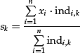
where xi is a factor and indi,k represent the weight of stock i in industry k. Next, we subtract the industry average of the industry scores, sk, from each stock. We compute
![]()
where xinew is the new industry neutral factor.
We can use linear regression to orthogonalize a factor. We first determine the coefficients in the equation
![]()
where fi is the factor to orthogonalize the factor xi by, b is the contribution of fi to xi, and εi is the component of the factor xi not related to fi. εi is orthogonal to fi (that is, εi is independent of fi) and represents the neutralized factor
![]()
In the same fashion, we can orthogonalize our variable relative to a set of factors by using the multivariate linear regression
![]()
and then setting xinew = εi.
Often portfolio managers use a risk model to forecast risk and an alpha model to forecast returns. The interaction between factors in a risk model and an alpha model often concerns portfolio managers. One possible approach to address this concern is to orthogonalize the factors or final scores from the alpha model against the factors used in the risk model. Later in the entry, we discuss this issue in more detail.
Transformation
It is common practice to apply transformations to data used in statistical and econometric models. In particular, factors are often transformed such that the resulting series is symmetric or close to being normally distributed. Frequently used transformations include natural logarithms, exponentials, and square roots. For example, a factor such as market capitalization has a large skew because a sample of large-cap stocks typically includes mega-capitalization stocks. To reduce the influence of mega-capitalization companies, we may instead use the natural logarithm of market capitalization in a linear regression model.
Outlier Detection and Management
Outliers are observations that seem to be inconsistent with the other values in a data set. Financial data contain outliers for a number of reasons including data errors, measurement errors, or unusual events. Interpretation of data containing outliers may therefore be misleading. For example, our estimates could be biased or distorted, resulting in incorrect conclusions.
Outliers can be detected by several methods. Graphs such as boxplots, scatter plots, or histograms can be useful to visually identify them. Alternatively, there are a number of numerical techniques available. One common method is to compute the interquartile-range and then identify outliers as those values that are some multiple of the range. The interquartile-range is a measure of dispersion and is calculated as the difference between the third and first quartiles of a sample. This measure represents the middle 50% of the data, removing the influence of outliers.
After outliers have been identified, we need to reduce their influence in our analysis. Trimming and winsorization are common procedures for this purpose. Trimming discards extreme values in the data set. This transformation requires the researcher to determine the direction (symmetric or asymmetric) and the amount of trimming to occur.
Winsorization is the process of transforming extreme values in the data. First, we calculate percentiles of the data. Next we define outliers by referencing a certain percentile ranking. For example, any data observation that is greater than the 97.5 percentile or less than the 2.5 percentile could be considered an outlier. Finally, we set all values greater or less than the reference percentile ranking to particular values. In our example, we may set all values greater than the 97.5 percentile to the 97.5 percentile value and all values less than 2.5 percentile set to the 2.5 percentile value. It is important to fully investigate the practical consequences of using either one of these procedures.
ANALYSIS OF FACTOR DATA
After constructing factors for all securities in the investable universe, each factor is analyzed individually. Presenting the time-series and cross-sectional averages of the mean, standard deviations, and key percentiles of the distribution provide useful information for understanding the behavior of the chosen factors.
Although we often rely on techniques that assume the underlying data generating process is normally distributed, or at least approximately, most financial data is not. The underlying data generating processes that embody aggregate investor behavior and characterize the financial markets are unknown and exhibit significant uncertainty. Investor behavior is uncertain because not all investors make rational decisions or have the same goals. Analyzing the properties of data may help us better understand how uncertainty affects our choice and calibration of a model.
Below we provide some examples of the cross-sectional characteristics of various factors. For ease of exposition we use histograms to evaluate the data rather than formal statistical tests. We let particular patterns or properties of the histograms guide us in the choice of the appropriate technique to model the factor. We recommend that an intuitive exploration should be followed by a more formal statistical testing procedure. Our approach here is to analyze the entire sample, all positive values, all negative values, and zero values. Although omitted here, a thorough analysis should also include separate subsample analysis.
Example 1: EBITDA/EV
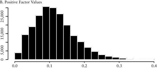
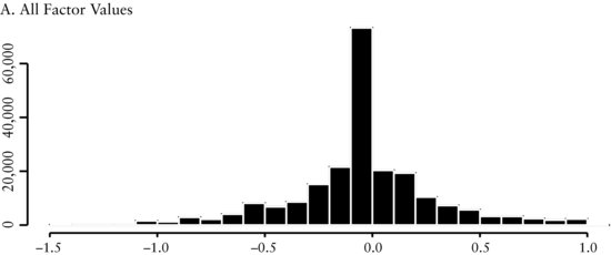
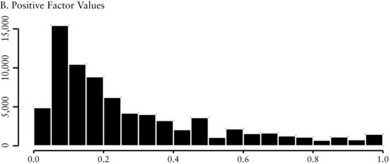
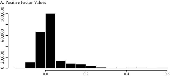
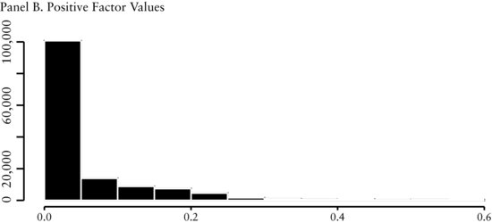
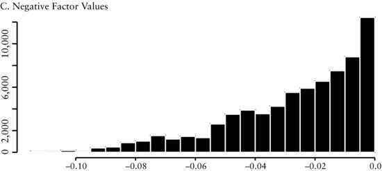
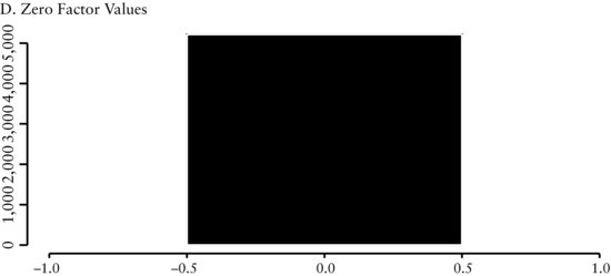
The first factor we discuss is the earnings before interest, taxes, and amortization to enterprise value (EBITDA/EV) factor. Enterprise value is calculated as the market value of the capital structure. This factor measures the price (enterprise value) investors pay to receive the cash flows (EBITDA) of a company. The economic intuition underlying this factor is that the valuation of a company’s cash flow determines the attractiveness of companies to an investor.
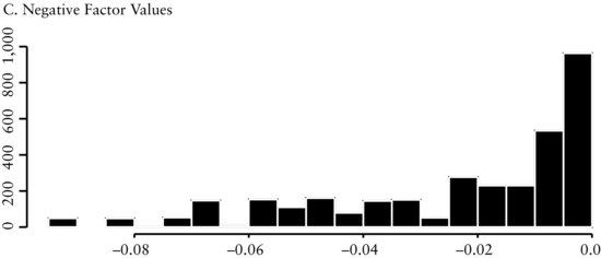
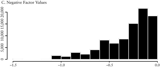
Figure 2(A) presents a histogram of all cross-sectional values of the EBITDA/EV factor throughout the entire history of the study. The distribution is close to normal, showing there is a fairly symmetric dispersion among the valuations companies receive. Figure 2(B) shows that the distribution of all the positive values of the factor is also almost normally distributed. On the other hand, Figure 2(C) shows that the distribution of the negative values is skewed to the left. However, because there are only a small number of negative values, it is likely that they will not greatly influence our model.
Example 2: Revisions
We evaluate the cross-sectional distribution of the earnings revisions factor.13 The revisions factor we use is derived from sell-side analyst earnings forecasts from the IBES database. The factor is calculated as the number of analysts who revise their earnings forecast upward minus the number of downward forecasts, divided by the total number of forecasts. The economic intuition underlying this factor is that there should be a positive relation to changes in forecasts of earnings and subsequent returns.
In Figure 3(A) we see that the distribution of revisions is symmetric and leptokurtic around a mean of about zero. This distribution ties with the economic intuition behind the revisions. Since business prospects of companies typically do not change from month-to-month, sell-side analysts will not revise their earnings forecast every month. Consequently, we expect and find the cross-sectional range to be peaked at zero. Figure 3(B) and (C), respectively, show there is a smaller number of both positive and negative earnings revisions and each one of these distributions are skewed.
Example 3: Share Repurchase
We evaluate the cross-sectional distribution of the shares repurchases factor. This factor is calculated as the difference of the current number of common shares outstanding and the number of shares outstanding 12 months ago, divided by the number of shares outstanding 12 months ago. The economic intuition underlying this factor is that share repurchase provides information to investors about future earnings and valuation of the company’s stock.14 We expect there to be a positive relationship between a reduction in shares outstanding and subsequent returns.
We see in Figure 4(A) that the distribution is leptokurtic. The positive values (see Fig-ure 4(B)) are skewed to the right and the negative values (see Figure 4(C)) are clustered in a small band. The economic intuition underlying share repurchases is the following. Firms with increasing share count indicate they require additional sources of cash. This need could be an early sign that the firm is experiencing higher operating risks or financial distress. We would expect these firms to have lower future returns. Firms with decreasing share count have excess cash and are returning value back to shareholders. Decreasing share count could result because management believes the shares are undervalued. As expected, we find the cross-sectional range to be peaked at zero (see Figure 4(D)) since not all firms issue or repurchase shares on a regular basis.

KEY POINTS
- A factor is a common characteristic among a group of assets. Factors should be founded on sound economic intuition, market insight, or an anomaly.
- Factors fall into three categories—macroeconomic, cross-sectional, and statistical factors.
- The main steps in the development of a factor-based trading strategy are (1) defining a trading idea or investment strategy, (2) developing factors, (3) acquiring and processing data, (4) analyzing the factors, (5) building the strategy, (6) evaluating the strategy, (7) backtesting the strategy, and (8) implementing the strategy.
- Most trading strategies are exposed to risk. The main sources of risk are fundamental risk, noise trader risk, horizon risk, model risk, implementation risk, and liquidity risk.
- Factors are often derived from company characteristics and metrics, and market data. Examples of company characteristics and metrics include valuation ratios, operating efficiency ratios, profitability ratios, and solvency ratios. Example of useful market data include analysts forecasts, prices and returns, and trading volume.
- High-quality data are critical to the success of a trading strategy. Model output is only as good as the data used to calibrate it.
- Some common data problems and biases are backfilling and restatements of data, missing data, inconsistently reported data, and survivorship and look-ahead biases.
- The ability to detect and adjust outliers is crucial to a quantitative investment process.
- Common methods used for adjusting data are standardization, orthogonalization, transformation, trimming, and winsorization.
- The statistical properties of factors need to be carefully analyzed. Basic statistical measures include the time-series and cross-sectional averages of the mean, standard deviations, and key percentiles.
NOTES
1. Graham and Dodd (1962).
2. Graham (1949).
3. See Bernstein (1992).
4. See Fama and French (1988).
5. See, for example, Menchero and Poduri (2008).
6. Thomson MarketQA, http://thomsonreuters.com/products_services/financial/financial_products/quantitative_analysis/quantitative_analytics.
7. Factset Research Systems, http://www.factset.com.
8. Compustat Xpressfeed, http://www.compustat.com.
9. See Barberis and Thaler (2003).
10. For a discussion of the sources of model misspecification and remedies, see Fabozzi, Focardi, and Kolm (2010).
11. The ability of EBITDA/EV to forecast future returns is discussed in, for example, Dechow, Kothari, and Watts (1988).
12. See Nagel (2001).
13. For a representative study see, for example, Bercel (1994).
14. See Grullon and Michaely (2004).
REFERENCES
Barberis, N., and Thaler, R. (2003). A survey of behavioral finance. In G. M. Constantinides, M. Harris, and R. M. Stulz (Eds.), Handbook of the Economics of Finance. Amsterdam: Elsevier Science.
Bercel, A. (1994). Consensus expectations and international equity returns. Financial Analysts Journal 50, 4: 76–80.
Bernstein, P. L. (1992). Capital Ideas: The Improbable Origins of Modern Wall Street. New York: The Free Press.
Bushee, B. J., and Raedy, J. S. (2006). Factors affecting the implementability of stock market trading strategies. Working paper, University of Pennsylvania and University of North Carolina.
Cerniglia, J. A., and Kolm, P. N. (2009). The information content of order in a tick-by-tick analysis of the equity market in August 2007. Working paper, Courant Institute, New York University.
Dechow, P. M., Kothari, S. P., and Watts, R. L. (1998). The relation between earnings and cash flows. Journal of Accounting and Economics 25, 2: 133–168.
Fabozzi, F. J., Focardi, S. M., and Kolm, P. N. (2010). Quantitative Equity Investing. Hoboken, NJ: John Wiley & Sons.
Fama, E. F., and French, K. R. (1988). Dividend yields and expected stock returns. Journal of Financial Economics 22, 1: 3–25.
Graham, B. (1973). The Intelligent Investor. New York: Harper & Row.
Graham, B., and Dodd, D. (1962). Security Analysis. New York: McGraw-Hill.
Grullon, G., and Michaely, R. (2004). The information content of share repurchase programs. Journal of Finance 59, 2: 651–680.
Khandani, A. E., and Lo, A. W. (2007). What happened to the quants in August 2007? Journal of Investment Management 5, 4: 5–54.
Kothari, S. P., Sabino, J. S., and Zach, T. (2005). Implications of survival and data trimming for tests of market efficiency. Journal of Accounting and Economics 39, 1: 129–161.
Menchero, J., and Poduri, V. (2008). Custom factor attribution. Financial Analysts Journal 62, 2: 81–92.
Nagel, S. (2001). Accounting information free of selection bias: A New UK database 1953–1999. Working paper, Stanford Graduate School of Business.