
Time Value of Money
In this entry, we introduce the mathematical process of translating a value today into a value at some future point in time, and then show how this process can be reversed to determine the value today of some future amount. We then show how to extend the time value of money mathematics to include multiple cash flows and the special cases of annuities and loan amortization. Finally, we demonstrate how these mathematics can be used to calculate the yield on an investment.1
IMPORTANCE OF THE TIME VALUE OF MONEY
The notion that money has a time value is one of the most basic concepts in investment analysis. Making decisions today regarding future cash flows requires understanding that the value of money does not remain the same throughout time.
A dollar today is worth less than a dollar some time in the future for two reasons:
One dollar one year from now is not as valuable as one dollar today. After all, you can invest a dollar today and earn interest so that the value it grows to next year is greater than the one dollar today. This means we have to take into account the time value of money to quantify the relation between cash flows at different points in time.
Expected cash flows may not materialize. Uncertainty stems from the nature of forecasts of the timing and/or the amount of cash flows. We do not know for certain when, whether, or how much cash flows will be in the future. This uncertainty regarding future cash flows must somehow be taken into account in assessing the value of an investment.
Translating a current value into its equivalent future value is referred to as compounding. Translating a future cash flow or value into its equivalent value in a prior period is referred to as discounting. This entry outlines the basic mathematical techniques used in compounding and discounting.
Suppose someone wants to borrow $100 today and promises to pay back the amount borrowed in one month. Would the repayment of only the $100 be fair? Probably not. There are two things to consider. First, if the lender didn’t lend the $100, what could he or she have done with it? Second, is there a chance that the borrower may not pay back the loan? So, when considering lending money, we must consider the opportunity cost (that is, what could have been earned or enjoyed), as well as the uncertainty associated with getting the money back as promised.
Let’s say that someone is willing to lend the money, but that they require repayment of the $100 plus some compensation for the opportunity cost and any uncertainty the loan will be repaid as promised. The amount of the loan, the $100, is the principal. The compensation required for allowing someone else to use the $100 is the interest.
Looking at this same situation from the perspective of time and value, the amount that you are willing to lend today is the loan’s present value. The amount that you require to be paid at the end of the loan period is the loan’s future value. Therefore, the future period’s value is comprised of two parts:
![]()
The interest is compensation for the use of funds for a specific period. It consists of (1) compensation for the length of time the money is borrowed and (2) compensation for the risk that the amount borrowed will not be repaid exactly as set forth in the loan agreement.
DETERMINING THE FUTURE VALUE
Suppose you deposit $1,000 into a savings account at the Surety Savings Bank and you are promised 10% interest per period. At the end of one period you would have $1,100. This $1,100 consists of the return of your principal amount of the investment (the $1,000) and the interest or return on your investment (the $100). Let’s label these values:
- $1,000 is the value today, the present value, PV.
- $1,100 is the value at the end of one period, the future value, FV.
- 10% is the rate interest is earned in one period, the interest rate, i.
To get to the future value from the present value:
This is equivalent to:
![]()
In terms of our example,
![]()
If the $100 interest is withdrawn at the end of the period, the principal is left to earn interest at the 10% rate. Whenever you do this, you earn simple interest. It is simple because it repeats itself in exactly the same way from one period to the next as long as you take out the interest at the end of each period and the principal remains the same. If, on the other hand, both the principal and the interest are left on deposit at the Surety Savings Bank, the balance earns interest on the previously paid interest, referred to as compound interest. Earning interest on interest is called compounding because the balance at any time is a combination of the principal, interest on principal, and interest on accumulated interest (or simply, interest on interest).
If you compound interest for one more period in our example, the original $1,000 grows to $1,210.00:
The present value of the investment is $1,000, the interest earned over two years is $210, and the future value of the investment after two years is $1,210.
The relation between the present value and the future value after two periods, breaking out the second period interest into interest on the principal and interest on interest, is:
or, collecting the PVs from each term and applying a bit of elementary algebra,
![]()
The balance in the account two years from now, $1,210, comprises three parts:
To determine the future value with compound interest for more than two periods, we follow along the same lines:
The value of N is the number of compounding periods, where a compounding period is the unit of time after which interest is paid at the rate i. A period may be any length of time: a minute, a day, a month, or a year. The important thing is to make sure the same compounding period is reflected throughout the problem being analyzed. The term “(1 + i)N” is referred to as the compound factor. It is the rate of exchange between present dollars and dollars N compounding periods into the future. Equation (1) is the basic valuation equation—the foundation of financial mathematics. It relates a value at one point in time to a value at another point in time, considering the compounding of interest.
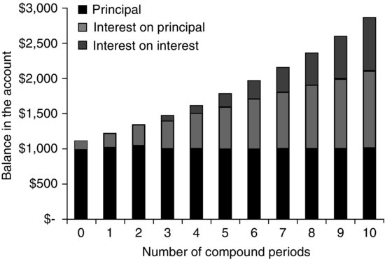
The relation between present and future values for a principal of $1,000 and interest of 10% per period through 10 compounding periods is shown graphically in Figure 1. For example, the value of $1,000, earning interest at 10% per period, is $2,593.70 ten periods into the future:
Figure 1 The Value of $1,000 Invested 10 Years in an Account That Pays 10% Compounded Interest per Year
![]()
As you can see in this figure the $2,593.70 balance in the account at the end of 10 periods is comprised of three parts:
We can express the change in the value of the savings balance (that is, the difference between the ending value and the beginning value) as a growth rate. A growth rate is the rate at which a value appreciates (a positive growth) or depreciates (a negative growth) over time. Our $1,000 grew at a rate of 10% per year over the 10-year period to $2,593.70. The average annual growth rate of our investment of $1,000 is 10%—the value of the savings account balance increased 10% per year.
We could also express the appreciation in our savings balance in terms of a return. A return is the income on an investment, generally stated as a change in the value of the investment over each period divided by the amount at the investment at the beginning of the period. We could also say that our investment of $1,000 provides an average annual return of 10% per year. The average annual return is not calculated by taking the change in value over the entire 10-year period ($2,593.70 − $1,000) and dividing it by $1,000. This would produce an arithmetic average return of 159.37% over the 10-year period, or 15.937% per year. But the arithmetic average ignores the process of compounding. The correct way of calculating the average annual return is to use a geometric average return:
which is a rearrangement of equation (1) Using the values from the example,
Therefore, the annual return on the invest-ment—sometimes referred to as the compound average annual return or the true return—is 10% per year.
Here is another example for calculating a future value. A common investment product of a life insurance company is a guaranteed investment contract (GIC). With this investment, an insurance company guarantees a specified interest rate for a period of years. Suppose that the life insurance company agrees to pay 6% annually for a five-year GIC and the amount invested by the policyholder is $10 million. The amount of the liability (that is, the amount this life insurance company has agreed to pay the GIC policyholder) is the future value of $10 million when invested at 6% interest for five years. In terms of equation (1), PV = $10,000,000, i = 6%, and N = 5, so that the future value is:
![]()
Compounding More Than One Time per Year
An investment may pay interest more than one time per year. For example, interest may be paid semiannually, quarterly, monthly, weekly, or daily, even though the stated rate is quoted on an annual basis. If the interest is stated as, say, 10% per year, compounded semiannually, the nominal rate—often referred to as the annual percentage rate (APR)—is 10%. The basic valuation equation handles situations in which there is compounding more frequently than once a year if we translate the nominal rate into a rate per compounding period. Therefore, an APR of 10% with compounding semiannually is 5% per period—where a period is six months—and the number of periods in one year is 2.
Consider a deposit of $50,000 in an account for five years that pays 8% interest, compounded quarterly. The interest rate per period, i, is 8%/4 = 2% and the number of compounding periods is 5 × 4 = 20. Therefore, the balance in the account at the end of five years is:
![]()
As shown in Figure 2, through 50 years with both annual and quarterly compounding, the investment’s value increases at a faster rate with the increased frequency of compounding.
Figure 2 Value of $50,000 Invested in the Account that Pays 8% Interest per Year: Quarterly versus Annual Compounding
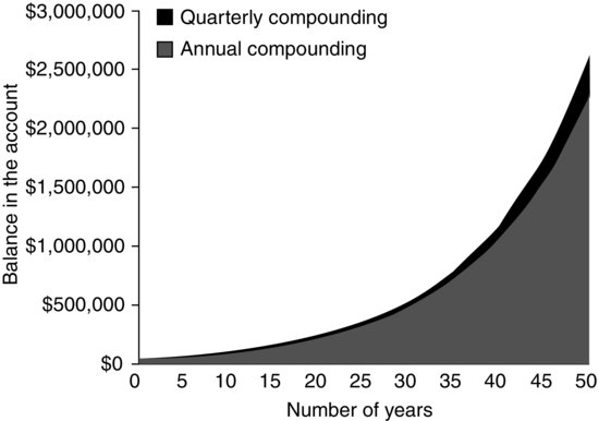
The last example illustrates the need to correctly identify the “period” because this dictates the interest rate per period and the number of compounding periods. Because interest rates are often quoted in terms of an APR, we need to be able to translate the APR into an interest rate per period and to adjust the number of periods. To see how this works, let’s use an example of a deposit of $1,000 in an account that pays interest at a rate of 12% per year, with interest compounded for different compounding frequencies. How much is in the account after, say, five years depends on the compounding frequency:
As you can see, both the rate per period, i, and the number of compounding periods, N, are adjusted and depend on the frequency of compounding. Interest can be compounded for any frequency, such as daily or hourly.
Let’s work through another example for compounding with compounding more than once a year. Suppose we invest $200,000 in an investment that pays 4% interest per year, compounded quarterly. What will be the future value of this investment at the end of 10 years?
The given information is i = 4%/4 = 1% and N = 10 × 4 = 40 quarters. Therefore,
![]()
Continuous Compounding
The extreme frequency of compounding is continuous compounding—interest is compounded instantaneously. The factor for compounding continuously for one year is eAPR, where e is 2.71828 … , the base of the natural logarithm. And the factor for compounding continuously for two years is eAPR eAPR or eAPR. The future value of an amount that is compounded continuously for N years is:
(3) ![]()
where APR is the annual percentage rate and eN(APR) is the compound factor.
If $1,000 is deposited in an account for five years with interest of 12% per year, compounded continuously,
![]()
Comparing this future value with that if interest is compounded annually at 12% per year for five years, $1,762.34, we see the effects of this extreme frequency of compounding.
Multiple Rates
In our discussion thus far, we have assumed that the investment will earn the same periodic interest rate, i. We can extend the calculation of a future value to allow for different interest rates or growth rates for different periods. Suppose an investment of $10,000 pays 9% during the first year and 10% during the second year. At the end of the first period, the value of the investment is $10,000 (1 + 0.09), or $10,900. During the second period, this $10,900 earns interest at 10%. Therefore, the future value of this $10,000 at the end of the second period is:
![]()
We can write this more generally as:
(4) ![]()
where iN is the interest rate for period N.
Consider a $50,000 investment in a one-year bank certificate of deposit (CD) today and rolled over annually for the next two years into one-year CDs. The future value of the $50,000 investment will depend on the one-year CD rate each time the funds are rolled over. Assuming that the one-year CD rate today is 5% and that it is expected that the one-year CD rate one year from now will be 6%, and the one-year CD rate two years from now will be 6.5%, then we know:
![]()
Continuing this example, what is the average annual interest rate over this period? We know that the future value is $59,267.25, the present value is $50,000, and N = 3:
![]()
which is also:
![]()
DETERMINING THE PRESENT VALUE
Now that we understand how to compute future values, let’s work the process in reverse. Suppose that for borrowing a specific amount of money today, the Yenom Company promises to pay lenders $5,000 two years from today. How much should the lenders be willing to lend Yenom in exchange for this promise? This dilemma is different than figuring out a future value. Here we are given the future value and have to figure out the present value. But we can use the same basic idea from the future value problems to solve present value problems.
If you can earn 10% on other investments that have the same amount of uncertainty as the $5,000 Yenom promises to pay, then:
- The future value, FV = $5,000.
- The number of compounding periods, N = 2.
- The interest rate, i = 10%.
We also know the basic relation between the present and future values:
![]()
Substituting the known values into this equation:
![]()
To determine how much you are willing to lend now, PV, to get $5,000 one year from now, FV, requires solving this equation for the unknown present value:
Therefore, you would be willing to lend $4,132.25 to receive $5,000 one year from today if your opportunity cost is 10%. We can check our work by reworking the problem from the reverse perspective. Suppose you invested $4,132.25 for two years and it earned 10% per year. What is the value of this investment at the end of the year?
We know: PV = $4,132.25, N = 10% or 0.10, and i = 2.
Therefore, the future value is:
![]()
Compounding translates a value in one point in time into a value at some future point in time. The opposite process translates future values into present values: Discounting translates a value back in time. From the basic valuation equation:
![]()
we divide both sides by (1 + i)N and exchange sides to get the present value,
(5) ![]()
![]()
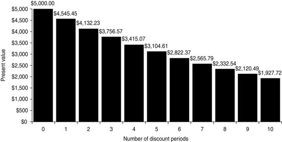
The term in brackets [ ] is referred to as the discount factor since it is used to translate a future value to its equivalent present value. The present value of $5,000 for discount periods ranging from 0 to 10 is shown in Figure 3.
Figure 3 Present Value of $5,000 Discounted at 10%
If the frequency of compounding is greater than once a year, we make adjustments to the rate per period and the number of periods as we did in compounding. For example, if the future value five years from today is $100,000 and the interest is 6% per year, compounded semiannually, i = 6%/2 = 3% and N = 5 × 2 = 10, and the present value is:
![]()
Here is an example of calculating a present value. Suppose that the goal is to have $75,000 in an account by the end of four years. And suppose that interest on this account is paid at a rate of 5% per year, compounded semiannually. How much must be deposited in the account today to reach this goal? We are given FV = $75,000, i = 5%/2 = 2.5% per six months, and N = 4 × 2 = 8 six-month periods. The amount of the required deposit is therefore:
![]()
DETERMINING THE UNKNOWN INTEREST RATE
As we saw earlier in our discussion of growth rates, we can rearrange the basic equation to solve for i:
![]()
As an example, suppose that the value of an investment today is $100 and the expected value of the investment in five years is expected to be $150. What is the annual rate of appreciation in value of this investment over the five-year period?
There are many applications in finance where it is necessary to determine the rate of change in values over a period of time. If values are increasing over time, we refer to the rate of change as the growth rate. To make comparisons easier, we usually specify the growth rate as a rate per year.
For example, if we wish to determine the rate of growth in these values, we solve for the unknown interest rate. Consider the growth rate of dividends for General Electric. General Electric pays dividends each year. In 1996, for example, General Electric paid dividends of $0.317 per share of its common stock, whereas in 2006 the company paid $1.03 in dividends per share. This represents a growth rate of 12.507%:
The 12.507% is the average annual rate of the growth during this 10-year span.
DETERMINING THE NUMBER OF COMPOUNDING PERIODS
Given the present and future values, calculating the number of periods when we know the interest rate is a bit more complex than calculating the interest rate when we know the number of periods. Nevertheless, we can develop an equation for determining the number of periods, beginning with the valuation formula given by equation (1) and rearranging to solve for N,
(6) ![]()
where ln indicates the natural logarithm, which is the log of the base e. (e is approximately equal to 2.718. The natural logarithm function can be found on most calculators, usually indicated by “ln”.)
Suppose that the present value of an investment is $100 and you wish to determine how long it will take for the investment to double in value if the investment earns 6% per year, compounded annually:
You’ll notice that we round off to the next whole period. To see why, consider this last example. After 11.8885 years, we have doubled our money if interest were paid 88.85% the way through the 12th year. But, we stated earlier that interest is paid at the and of each period—not part of the way through. At the end of the 11th year, our investment is worth $189.93, and at the end of the 12th year, our investment is worth $201.22. So, our investment’s value doubles by the 12th period—with a little extra, $1.22.
THE TIME VALUE OF A SERIES OF CASH FLOWS
Applications in finance may require the determination of the present or future value of a series of cash flows rather than simply a single cash flow. The principles of determining the future value or present value of a series of cash flows are the same as for a single cash flow, yet the math becomes a bit more cumbersome.
Suppose that the following deposits are made in a Thrifty Savings and Loan account paying 5% interest, compounded annually:
| Time When Deposit Is Made | Amount of Deposit |
| Today | $1,000 |
| At the end of the first year | 2,000 |
| At the end of the second year | 1,500 |
What is the balance in the savings account at the end of the second year if no withdrawals are made and interest is paid annually?
Let’s simplify any problem like this by referring to today as the end of period 0, and identifying the end of the first and each successive period as 1, 2, 3, and so on. Represent each end-of-period cash flow as “CF” with a subscript specifying the period to which it corresponds. Thus, CF0 is a cash flow today, CF10 is a cash flow at the end of period 10, and CF25 is a cash flow at the end of period 25, and so on.
Representing the information in our example using cash flow and period notation:
| Period | Cash Flow | End-of-Period Cash Flow |
| 0 | CF0 | $1,000 |
| 1 | CF1 | $2,000 |
| 2 | CF2 | $1,500 |
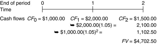
The future value of the series of cash flows at the end of the second period is calculated as follows:
The last cash flow, $1,500, was deposited at the very end of the second period—the point of time at which we wish to know the future value of the series. Therefore, this deposit earns no interest. In more formal terms, its future value is precisely equal to its present value.
Today, the end of period 0, the balance in the account is $1,000 since the first deposit is made but no interest has been earned. At the end of period 1, the balance in the account is $3,050, made up of three parts:
The balance in the account at the end of period 2 is $4,702.50, made up of five parts:
These cash flows can also be represented in a time line. A time line is used to help graphically depict and sort out each cash flow in a series. The time line for this example is shown in Figure 4. From this example, you can see that the future value of the entire series is the sum of each of the compounded cash flows comprising the series. In much the same way, we can determine the future value of a series comprising any number of cash flows. And if we need to, we can determine the future value of a number of cash flows before the end of the series.
Figure 4 Time Line for the Future Value of a Series of Uneven Cash Flows Deposited to Earn 5% Compounded Interest per Period
For example, suppose you are planning to deposit $1,000 today and at the end of each year for the next ten years in a savings account paying 5% interest annually. If you want to know the future value of this series after four years, you compound each cash flow for the number of years it takes to reach four years. That is, you compound the first cash flow over four years, the second cash flow over three years, the third over two years, the fourth over one year, and the fifth you don’t compound at all because you will have just deposited it in the bank at the end of the fourth year.
To determine the present value of a series of future cash flows, each cash flow is discounted back to the present, where the beginning of the first period, today, is designated as 0. As an example, consider the Thrifty Savings & Loan problem from a different angle. Instead of calculating what the deposits and the interest on these deposits will be worth in the future, let’s calculate the present value of the deposits. The present value is what these future deposits are worth today.
In the series of cash flows of $1,000 today, $2,000 at the end of period 1, and $1,500 at the end of period 2, each are discounted to the present, 0, as follows:
The present value of the series is the sum of the present value of these three cash flows, $4,265.30. For example, the $1,500 cash flow at the end of period 2 is worth $1,428.57 at the end of the first period and is worth $1,360.54 today.
The present value of a series of cash flows can be represented in notation form as:
For example, if there are cash flows today and at the end of periods 1 and 2, today’s cash flow is not discounted, the first period cash flow is discounted one period, and the second period cash flow is discounted two periods.
We can represent the present value of a series using summation notation as shown below:
(7) ![]()
This equation tells us that the present value of a series of cash flows is the sum of the products of each cash flow and its corresponding discount factor.
Shortcuts: Annuities
There are valuation problems that require us to evaluate a series of level cash flows—each cash flow is the same amount as the others—received at regular intervals. Let’s suppose you expect to deposit $2,000 at the end of each of the next four years in an account earning 8% compounded interest. How much will you have available at the end of the fourth year?
As we just did for the future value of a series of uneven cash flows, we can calculate the future value (as of the end of the fourth year) of each $2,000 deposit, compounding interest at 8%:
Figure 5 shows the contribution of each deposit and the accumulated interest at the end of each period.
Figure 5 Balance in an Account in Which Deposits of $2,000 Each Are Made Each Year (The Balance in the Account Earns 8%)
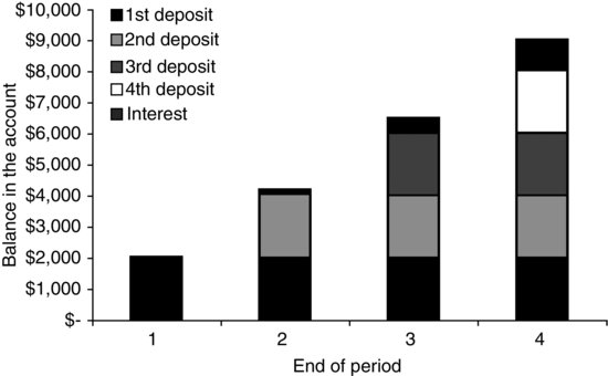
- At the end of the first year, there is $2,000.00 in the account because you have just made your first deposit.
- At the end of the second, there is $4,160.00 in the account: two deposits of $2,000 each, plus $160 interest (8% of $2,000).
- At the end of the third year, there is $6,492.80 in the account: three deposits of $2,000.00 each, plus accumulated interest of $492.80 [$160.00 + (0.08 × $4,000) + (0.08 × $160)].
- At the end of the fourth year, you would have $9,012.20 available: four deposits of $2,000 each, plus $1,012.20 accumulated interest [$160.00 + $492.80 + (0.08 × $6,000) + (0.08 × ($160.00 + 492.80)].
Notice that in our calculations, each deposit of $2,000 is multiplied by a factor that corresponds to an interest rate of 8% and the number of periods that the deposit has been in the savings account. Since the deposit of $2,000 is common to each multiplication, we can simplify the math a bit by multiplying the $2,000 by the sum of the factors to get the same answer:
A series of cash flows of equal amount occurring at even intervals is referred to as an annuity. Determining the value of an annuity, whether compounding or discounting, is simpler than valuing uneven cash flows. If each CFt is equal (that is, all the cash flows are the same value) and the first one occurs at the end of the first period (t = 1), we can express the future value of the series as:
![]()
N is last and t indicates the time period corresponding to a particular cash flow, starting at 1 for an ordinary annuity. Since CFt is shorthand for: CF1, CF2, CF3, … , CFN, and we know that CF1 = CF2 = CF3 = … CFN, let’s make things simple by using CF to indicate the same value for the periodic cash flows. Rearranging the future value equation we get:
This equation tells us that the future value of a level series of cash flows, occurring at regular intervals beginning one period from today (notice that t starts at 1), is equal to the amount of cash flow multiplied by the sum of the compound factors.
In a like manner, the equation for the present value of a series of level cash flows beginning after one period simplifies to:
![]()
or
This equation tells us that the present value of an annuity is equal to the amount of one cash flow multiplied by the sum of the discount factors.
Equations (8) and (9) are the valuation—future and present value—formulas for an ordinary annuity. An ordinary annuity is a special form of annuity, where the first cash flow occurs at the end of the first period.
To calculate the future value of an annuity we multiply the amount of the annuity (that is, the amount of one periodic cash flow) by the sum of the compound factors. The sum of these compounding factors for a given interest rate, i, and number of periods, N, is referred to as the future value annuity factor. Likewise, to calculate the present value of an annuity we multiply one cash flow of the annuity by the sum of the discount factors. The sum of the discounting factors for a given i and N is referred to as the present value annuity factor.
Suppose you wish to determine the future value of a series of deposits of $1,000, deposited each year in the No Fault Vault Bank for five years, with the first deposit made at the end of the first year. If the NFV Bank pays 5% interest on the balance in the account at the end of each year and no withdrawals are made, what is the balance in the account at the end of the five years?
Each $1,000 is deposited at a different time, so it contributes a different amount to the future value. For example, the first deposit accumulates interest for four periods, contributing $1,215.50 to the future value (at the end of period 5), whereas the last deposit contributes only $1,000 to the future value since it is deposited at exactly the point in time when we are determining the future value, hence there is no interest on this deposit.
The future value of an annuity is the sum of the future value of each deposit:
The future value of the series of $1,000 deposits, with interest compounded at 5%, is $5,525.60. Since we know the value of one of the level period flows is $1,000, and the future value of the annuity is $5,525.60, and looking at the sum of the individual compounding factors, 5.5256, we can see that there is an easier way to calculate the future value of an annuity. If the sum of the individual compounding factors for a specific interest rate and a specific number of periods were available, all we would have to do is multiply that sum by the value of one cash flow to get the future value of the entire annuity.
In this example, the shortcut is multiplying the amount of the annuity, $1,000, by the sum of the compounding factors, 5.5256:
![]()
For large numbers of periods, summing the individual factors can be a bit clumsy—with possibilities of errors along the way. An alternative formula for the sum of the compound factors—that is, the future value annuity factor—is:
(10) ![]()
In the last example, N = 5 and i = 5%:
Let’s use the long method to find the present value of the series of five deposits of $1,000 each, with the first deposit at the end of the first period. Then we’ll do it using the shortcut method. The calculations are similar to the future value of an ordinary annuity, except we are taking each deposit back in time, instead of forward:
The present value of this series of five deposits is $4,329.40.
This same value is obtained by multiplying the annuity amount of $1,000 by the sum of the discounting factors, 4.3294:
![]()
Another, more convenient way of solving for the present value of an annuity is to rewrite the factor as:
(11) 
If there are many discount periods, this formula is a bit easier to calculate. In our last example,
which is different from the sum of the factors, 4.3294, due to rounding.
We can turn this present value of an annuity problem around to look at it from another angle. Suppose you borrow $4,329.40 at an interest rate of 5% per period and are required to pay back this loan in five installments (N = 5): one payment per period for five periods, starting one period from now. The payments are determined by equating the present value with the product of the cash flow and the sum of the discount factors:
substituting the known present value,
![]()
and rearranging to solve for the payment:
![]()
We can convince ourselves that five installments of $1,000 each can pay off the loan of $4,329.40 by carefully stepping through the calculation of interest and the reduction of the principal:
For example, the first payment of $1,000 is used to: (1) pay interest on the loan at 5% ($4,329.40 × 0.05 = $216.47) and (2) pay down the principal or loan balance ($1,000.00 − $216.47 = $783.53 paid off). Each successive payment pays off a greater amount of the loan—as the principal amount of the loan is reduced, less of each payment goes to paying off interest and more goes to reducing the loan principal. This analysis of the repayment of a loan is referred to as loan amortization. Loan amortization is the repayment of a loan with equal payments, over a specified period of time. As we can see from the example of borrowing $4,329.40, each payment can be broken down into its interest and principal components.
VALUING CASH FLOWS WITH DIFFERENT TIME PATTERNS
Valuing a Perpetual Stream of Cash Flows
There are some circumstances where cash flows are expected to continue forever. For example, a corporation may promise to pay dividends on preferred stock forever, or, a company may issue a bond that pays interest every six months, forever. How do you value these cash flow streams? Recall that when we calculated the present value of an annuity, we took the amount of one cash flow and multiplied it by the sum of the discount factors that corresponded to the interest rate and number of payments. But what if the number of payments extends forever—into infinity?
A series of cash flows that occur at regular intervals, forever, is a perpetuity. Valuing a perpetual cash flow stream is just like valuing an ordinary annuity. It looks like this:
Simplifying, recognizing that the cash flows CFt are the same in each period, and using summation notation,
![]()
As the number of discounting periods approaches infinity, the summation approaches 1/i. To see why, consider the present value annuity factor for an interest rate of 10%, as the number of payments goes from 1 to 200:
| Number of Discounting | Present Value |
| Periods, N | Annuity Factor |
| 1 | 0.9091 |
| 10 | 6.1446 |
| 40 | 9.7791 |
| 100 | 9.9993 |
| 200 | 9.9999 |
For greater numbers of payments, the factor approaches 10, or 1/0.10. Therefore, the present value of a perpetual annuity is very close to:
(12) ![]()
Suppose you are considering an investment that promises to pay $100 each period forever, and the interest rate you can earn on alternative investments of similar risk is 5% per period. What are you willing to pay today for this investment?
![]()
Therefore, you would be willing to pay $2,000 today for this investment to receive, in return, the promise of $100 each period forever.
Let’s look at the value of a perpetuity another way. Suppose that you are given the opportunity to purchase an investment for $5,000 that promises to pay $50 at the end of every period forever. What is the periodic interest per period—the return—associated with this investment?
We know that the present value is PV = $5,000 and the periodic, perpetual payment is CF = $50. Inserting these values into the formula for the present value of a perpetuity:
![]()
Solving for i,
![]()
Therefore, an investment of $5,000 that generates $50 per period provides 1% compounded interest per period.
Valuing an Annuity Due
The ordinary annuity cash flow analysis assumes that cash flows occur at the end of each period. However, there is another fairly common cash flow pattern in which level cash flows occur at regular intervals, but the first cash flow occurs immediately. This pattern of cash flows is called an annuity due. For example, if you win the Florida Lottery Lotto grand prize, you will receive your winnings in 20 installments (after taxes, of course). The 20 installments are paid out annually, beginning immediately. The lottery winnings are therefore an annuity due.
Like the cash flows we have considered thus far, the future value of an annuity due can be determined by calculating the future value of each cash flow and summing them. And, the present value of an annuity due is determined in the same way as a present value of any stream of cash flows.
Let’s consider first an example of the future value of an annuity due, comparing the values of an ordinary annuity and an annuity due, each comprising three cash flows of $500, compounded at the interest rate of 4% per period. The calculation of the future value of both the ordinary annuity and the annuity due at the end of three periods is:
| Ordinary annuity | Annuity due |
The future value of each of the $500 payments in the annuity due calculation is compounded for one more period than for the ordinary annuity. For example, the first deposit of $500 earns interest for two periods in the ordinary annuity situation [$500 (1 + 0.04)2], whereas the first $500 in the annuity due case earns interest for three periods [$500 (1 + 0.04)3].
In general terms,
(13) ![]()
which is equal to the future value of an ordinary annuity multiplied by a factor of 1 + i:
![]()
The present value of the annuity due is calculated in a similar manner, adjusting the ordinary annuity formula for the different number of discount periods:
(14) ![]()
Since the cash flows in the annuity due situation are each discounted one less period than the corresponding cash flows in the ordinary annuity, the present value of the annuity due is greater than the present value of the ordinary annuity for an equivalent amount and number of cash flows. Like the future value an annuity due, we can specify the present value in terms of the ordinary annuity factor:
![]()
Valuing a Deterred Annuity
A deferred annuity has a stream of cash flows of equal amounts at regular periods starting at some time after the end of the first period. When we calculated the present value of an annuity, we brought a series of cash flows back to the beginning of the first period—or, equivalently the end of the period 0. With a deferred annuity, we determine the present value of the ordinary annuity and then discount this present value to an earlier period.
To illustrate the calculation of the present value of an annuity due, suppose you deposit $20,000 per year in an account for 10 years, starting today, for a total of 10 deposits. What will be the balance in the account at the end of 10 years if the balance in the account earns 5% per year? The future value of this annuity due is:
Suppose you want to deposit an amount today in an account such that you can withdraw $5,000 per year for four years, with the first withdrawal occurring five years from today. We can solve this problem in two steps:
The first step requires determining the present value of a four-cash-flow ordinary annuity of $5,000. This calculation provides the present value as of the end of the fourth year (one period prior to the first withdrawal):
This means that there must be a balance in the account of $18,149.48 at the end of the fourth period to satisfy the withdrawals of $5,000 per year for four years.
The second step requires discounting the $18,149.48—the savings goal—to the present, providing the deposit today that produces the goal:
![]()
The balance in the account throughout the entire eight-year period is shown in Figure 6 with the balance indicated both before and after the $5,000 withdrawals.
Figure 6 Balance in the Account that Requires a Deposit Today (Year 0) that Permits Withdrawals of $5,000 Each Starting at the End of Year 5

Let’s look at a more complex deferred annuity. Consider making a series of deposits, beginning today, to provide for a steady cash flow beginning at some future time period. If interest is earned at a rate of 4% compounded per year, what amount must be deposited in a savings account each year for four years, starting today, so that $1,000 may be withdrawn each year for five years, beginning five years from today? As with any deferred annuity, we need to perform this calculation in steps:
The present value of the annuity deferred to the end of the fourth period is
Therefore, there must be $4,451.80 in the account at the end of the fourth year to permit five $1,000 withdrawals at the end of each of the years 5, 6, 7, 8, and 9.
The present value of the annuity at the end of the fourth year, $4,451.80, is the future value of the annuity due of four payments of an unknown amount. Using the formula for the future value of an annuity due,
and rearranging,
![]()
Therefore, by depositing $1,008.02 today and the same amount on the same date each of the next three years, we will have a balance in the account of $4,451.80 at the end of the fourth period. With this period 4 balance, we will be able to withdraw $1,000 at the end of the following five periods.
LOAN AMORTIZATION
There are securities backed by various types of loans. These include asset-backed securities, residential mortgage-backed securities, and commercial mortgage-backed securities. Consequently, it is important to understand the mathematics associated with loan amortization.
If an amount is loaned and then repaid in installments, we say that the loan is amortized. Therefore, loan amortization is the process of calculating the loan payments that amortize the loaned amount. We can determine the amount of the loan payments once we know the frequency of payments, the interest rate, and the number of payments.
Consider a loan of $100,000. If the loan is repaid in 24 annual installments (at the end of each year) and the interest rate is 5% per year, we calculate the amount of the payments by applying the relationship:
We want to solve for the loan payment, that is, the amount of the annuity. Using a financial calculator or spreadsheet, the periodic loan payment is $7,247.09 (PV = $100,000; N = 24; i = 5%). Therefore, the monthly payments are $7,247.09 each. In other words, if payments of $7,247.09 are made each year for 24 years (at the end of each year), the $100,000 loan will be repaid and the lender earns a return that is equivalent to a 5% interest on this loan.
We can calculate the amount of interest and principal repayment associated with each loan payment using a loan amortization schedule, as shown in Table 1.
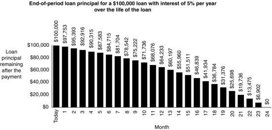
The loan payments are determined such that after the last payment is made there is no loan balance outstanding. Thus, the loan is referred to as a fully amortizing loan. Even though the loan payment each year is the same, the proportion of interest and principal differs with each payment: The interest is 5% of the principal amount of the loan that remains at the beginning of the period, whereas the principal repaid with each payment is the difference between the payment and the interest. As the payments are made, the remainder is applied to repayment of the principal; this is referred to as the scheduled principal repayment or the amortization. As the principal remaining on the loan declines, less interest is paid with each payment. We show the decline in the loan’s principal graphically in Figure 7. The decline in the remaining principal is not a linear, but is curvilinear due to the compounding of interest.
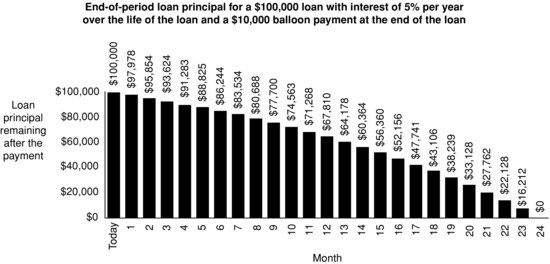
Loan amortization works the same whether this is a mortgage loan, a term loan, or any other loan in which the interest paid is determined on the basis of the remaining amount of the loan. The calculation of the loan amortization can be modified to suit different principal repayments, such as additional lump-sum payments, known as balloon payments. For example, if there is a $10,000 balloon payment at the end of the loan in the loan of $100,000 repaid over 24 years, the calculation of the payment is modified as:
Table 1 Loan Amortization on a $100,000 Loan for 24 Years and an Interest Rate of 5% per Year
Figure 7 Loan Amortization
The loan payment that solves this equation is $7,022.38 (PV = $100,000; N = 24; i = 5%; FV = $10,000). The last payment (that is, at the end of the 24th year) is the regular payment of $7,022.38, plus the balloon payment, for a total of $17,022.38. As you can see in Figure 8, the loan amortization is slower when compared to the loan without the balloon payment.
Figure 8 Loan Amortization with Balloon Payment
The same mathematics work with term loans. Term loans are usually repaid in installments either monthly, quarterly, semiannually, or annually. Let’s look at the typical repayment schedule for a term loan. Suppose that BigRock Corporation seeks a four-year term loan of $100 million. Let’s assume for now that the term loan carries a fixed interest rate of 8% and that level payments are made monthly. If the annual interest rate is 8%, the rate per month is 8% ÷ 12 = 0.6667% per month. In a typical term loan, the payments are structured such that the loan is fully amortizing.
For this four-year, $100 million term loan with an 8% interest rate, the monthly payment is $2,441,292.23 (PV = $100,000,000; N = 48; i = 06667%). This amount is determined by solving for the annuity payment that equates the present value of the payments with the amount of the loan, considering a discount rate of 0.6667%. In Table 2 we show for each month the beginning monthly balance, the interest payment for the month, the amount of the monthly, and the ending loan balance. Notice that in our illustration, the ending loan balance is zero. That is, it is a fully amortizing loan.
In the loan amortization examples so far, we have assumed that the interest rate is fixed throughout the loan. However, in many loans the interest rate may change during the loan, as in the case of a floating-rate loan. The new loan rate at the reset date is determined by a formula. The formula is typically composed of two parts. The first is the reference rate. For example, in a monthly pay loan, the loan rate might be one-month London Interbank Offered Rate (LIBOR). The second part is a spread that is added to the reference rate. This spread is referred to as the quoted margin and depends on the credit of the borrower.
A floating-rate loan requires a recalculation of the loan payment and payment schedule at each time the loan rate is reset. Suppose in the case of BigRock’s term loan that the rate remains constant for the first three years, but is reset to 9% in the fourth year. This requires BigRock to pay off the principal remaining at the end of three years, the $28,064,562.84, in the remaining 12 payments. The revised schedule of payments and payoff for the fourth year require a payment of $2,454,287.47 (PV = $27,064,562.84; N = 12; i = 0.09 ÷ 12 = 0.75%), as shown in Table 3.
Table 2 Term Loan Schedule: Fixed Rate, Fully Amortized
Table 3 Term Loan Schedule: Reset Rate, Fully Amortized
THE CALCULATION OF INTEREST RATES AND YIELDS
The calculation of the present or future value of a lump-sum or set of cash flows requires information on the timing of cash flows and the compound or discount rate. However, there are many applications in which we are presented with values and cash flows, and wish to calculate the yield or implied interest rate associated with these values and cash flows. By calculating the yield or implied interest rate, we can then compare investment or financing opportunities. We first look at how interest rates are stated and how the effective interest rate can be calculated based on this stated rate, and then we look at how to calculate the yield, or rate of return, on a set of cash flows.
Annual Percentage Rate versus Effective Annual Rate
A common problem in finance is comparing alternative financing or investment opportunities when the interest rates are specified in a way that makes it difficult to compare terms. The Truth in Savings Act requires institutions to provide the annual percentage yield for savings accounts. As a result of this law, consumers can compare the yields on different savings arrangements. But this law does not apply beyond savings accounts. One investment may pay 10% interest compounded semiannually, whereas another investment may pay 9% interest compounded daily. One financing arrangement may require interest compounding quarterly, whereas another may require interest compounding monthly. To compare investments or financing with different frequencies of compounding, we must first translate the stated interest rates into a common basis. There are two ways to convert interest rates stated over different time intervals so that they have a common basis: the annual percentage rate and the effective annual interest rate.
One obvious way to represent rates stated in various time intervals on a common basis is to express them in the same unit of time—so we annualize them. The annualized rate is the product of the stated rate of interest per compound period and the number of compounding periods in a year. Let i be the rate of interest per period and n be the number of compounding periods in a year. The annualized rate, also referred to as the nominal interest rate or the annual percentage rate (APR) is:
![]()
Consider the following example. Suppose the Lucky Break Loan Company has simple loan terms: Repay the amount borrowed, plus 50%, in six months. Suppose you borrow $10,000 from Lucky. After six months, you must pay back the $10,000 plus $5,000. The APR on financing with Lucky is the interest rate per period (50% for six months) multiplied by the number of compound periods in a year (two six-month periods in a year). For the Lucky Break financing arrangement:
![]()
But what if you cannot pay Lucky back after six months? Lucky will let you off this time, but you must pay back the following at the end of the next six months:
- The $10,000 borrowed.
- The $5,000 interest from the first six months.
- The 50% of interest on both the unpaid $10,000 and the unpaid $5,000 interest ($15,000 (0.50) = $7,500).
So, at the end of the year, knowing what is good for you, you pay off Lucky:
| Amount of the original loan | $10,000 |
| Interest from first six months | 5,000 |
| Interest on second six months | 7,500 |
| Total payment at end of the year | $22,500 |
Using the Lucky Break method of financing, you have to pay $12,500 interest to borrow $10,000 for one year’s time. Because you have to pay $12,500 interest to borrow $10,000 over one year’s time, you pay not 100% interest, but rather 125% interest per year ($12,500/$10,000 = 1.25 = 125%). What’s going on here? It looks like the APR in the Lucky Break example ignores the compounding (interest on interest) that takes place after the first six months. And that’s the way it is with all APRs. The APR ignores the effect of compounding. Therefore, this rate understates the true annual rate of interest if interest is compounded at any time prior to the end of the year. Nevertheless, APR is an acceptable method of disclosing interest on many lending arrangements, since it is easy to understand and simple to compute. However, because it ignores compounding, it is not the best way to convert interest rates to a common basis.
Another way of converting stated interest rates to a common basis is the effective rate of interest. The effective annual rate (EAR) is the true economic return for a given time period—it takes into account the compounding of interest—and is also referred to as the effective rate of interest.
Using our Lucky Break example, we see that we must pay $12,500 interest on the loan of $10,000 for one year. Effectively, we are paying 125% annual interest. Thus, 125% is the effective annual rate of interest. In this example, we can easily work through the calculation of interest and interest on interest. But for situations where interest is compounded more frequently, we need a direct way to calculate the effective annual rate. We can calculate it by resorting once again to our basic valuation equation:
![]()
Next, we consider that a return is the change in the value of an investment over a period and an annual return is the change in value over a year. Using our basic valuation equation, the relative change in value is the difference between the future value and the present value, divided by the present value:
![]()
Canceling PV from both the numerator and the denominator,
(15) ![]()
Let’s look how the EAR is affected by the compounding. Suppose that the Safe Savings and Loan promises to pay 6% interest on accounts, compounded annually. Since interest is paid once, at the end of the year, the effective annual return, EAR, is 6%. If the 6% interest is paid on a semiannual basis—3% every six months—the effective annual return is larger than 6% since interest is earned on the 3% interest earned at the end of the first six months. In this case, to calculate the EAR, the interest rate per compounding period—six months—is 0.03 (that is, 0.06/2) and the number of compounding periods in an annual period is 2:
![]()
Extending this example to the case of quarterly compounding with a nominal interest rate of 6%, we first calculate the interest rate per period, i, and the number of compounding periods in a year, n:
![]()
The EAR is:
![]()
As we saw earlier, the extreme frequency of compounding is continuous compounding. Continuous compounding is when interest is compounded at the smallest possible increment of time. In continuous compounding, the rate per period becomes extremely small:
![]()
And the number of compounding periods in a year, n, is infinite. The EAR is therefore:
(16) ![]()
where e is the natural logarithmic base.
For the stated 6% annual interest rate compounded continuously, the EAR is:
![]()
The relation between the frequency of compounding for a given stated rate and the effective annual rate of interest for this example indicates that the greater the frequency of compounding, the greater the EAR.
| Frequency of | Effective | |
| Compounding | Calculation | Annual Rate |
| Annual | (1 + 0.060)1 − 1 | 6.00% |
| Semiannual | (1 + 0.030)2 − 1 | 6.09% |
| Quarterly | (1 + 0.015)4 − 1 | 6.14% |
| Continuous | e0.06 − 1 | 6.18% |
Figuring out the effective annual rate is useful when comparing interest rates for different investments. It doesn’t make sense to compare the APRs for different investments having a different frequency of compounding within a year. But since many investments have returns stated in terms of APRs, we need to understand how to work with them.
To illustrate how to calculate effective annual rates, consider the rates offered by two banks, Bank A and Bank B. Bank A offers 9.2% compounded semiannually and Bank B other offers 9% compounded daily. We can compare these rates using the EARs. Which bank offers the highest interest rate? The effective annual rate for Bank A is (1 + 0.046)2 − 1 = 9.4%. The effective annual rate for Bank B is (1 + 0.000247)365 − 1 = 9.42%. Therefore, Bank B offers the higher interest rate.
Yields on Investments
Suppose an investment opportunity requires an investor to put up $1 million and offers cash inflows of $500,000 after one year and $600,000 after two years. The return on this investment, or yield, is the discount rate that equates the present values of the $500,000 and $600,000 cash inflows to equal the present value of the $1 million cash outflow. This yield is also referred to as the internal rate of return (IRR) and is calculated as the rate that solves the following:
![]()
Unfortunately, there is no direct mathematical solution (that is, closed-form solution) for the IRR, but rather we must use an iterative procedure. Fortunately, financial calculators and financial software ease our burden in this calculation. The IRR that solves this equation is 6.3941%:
![]()
In other words, if you invest $1 million today and receive $500,000 in one year and $600,000 in two years, the return on your investment is 6.3941%.
Another way of looking at this same yield is to consider that an investment’s IRR is the discount rate that makes the present value of all expected future cash flows—both the cash outflows for the investment and the subsequent inflows—equal to zero. We can represent the IRR as the rate that solves:
![]()
Consider another example. Suppose an investment of $1 million produces no cash flow in the first year but cash flows of $200,000, $300,000, and $900,000 two, three, and four years from now, respectively. The IRR for this investment is the discount rate that solves:
Using a calculator or a computer, we get the precise answer of 10.172% per year.
We can use this approach to calculate the yield on any type of investment, as long as we know the cash flows—both positive and negative—and the timing of these flows. Consider the case of the yield to maturity on a bond. Most bonds pay interest semiannually—that is, every six months. Therefore, when calculating the yield on a bond, we must consider the timing of the cash flows to be such that the discount period is six months.
Consider a bond that has a current price of 90; that is, if the par value of the bond is $1,000, the bond’s price is 90% of $1,000 or $900. And suppose that this bond has five years remaining to maturity and an 8% coupon rate. With five years remaining to maturity, the bond has 10 six-month periods remaining.With a coupon rate of 8%, this means that the cash flows for interest is $40 every six months. For a given bond, we therefore have the following information:
The six-month yield, rd, is the discount rate that solves the following:
![]()
Using a calculator or spreadsheet, the six-month yield is 5.315%. Bond yields are generally stated on the basis of an annualized yield, referred to as the yield to maturity (YTM) on a bond-equivalent basis. This YTM is analogous to the APR with semiannual compounding. Therefore, yield to maturity is 10.63%.
KEY POINTS
- A present value can be translated into a value in the future through compounding. The extreme frequency of compounding is continuous compounding.
- A future value can be converted into an equivalent value today through discounting.
- Applications in finance may require the determination of the present or future value of a series of cash flows rather than simply a single cash flow. The principles of determining the future value or present value of a series of cash flows are the same as for a single cash flow. That is, any number of cash flows can be translated into a present or future value.
- When faced with a series of cash flows, a financial modeler must value each cash flow individually, and then sum these individual values to arrive at the present value of the series.
- The tools of the time value of money can be used to value many different patterns of cash flows, including perpetuities, annuities due, and deferred annuities. Applying the tools to these different patterns of cash flows requires specifying the timing of the various cash flows.
- The interest on alternative investments is stated in different terms, so these interest rates must be placed on a common basis so that investment alternatives can be compared. Typically, an interest rate on an annual basis is specified, using either the annual percentage rate or the effective annual rate. The latter method is preferred since it takes into consideration the compounding of interest within a year.
- The yield on an investment (also referred to as internal rate of return) is the interest rate that makes the present value of the future cash flows equal to the cost of the investment.
NOTE
1. For a more detailed treatment of this topic, see Drake and Fabozzi (2009). The topic is covered in finite mathematics textbooks. See, for example, Barnett, Ziegler, and Byleen (2002), Mizrahi and Sullivan (1999), and Rolf (2007).
REFERENCES
Barnett, R.A., Ziegler, M.R., and Byleen, K.E. (2002). Finite Mathematics for Business, Economics, Life Sciences, and Social Sciences, 9th ed. Upper Saddle River, NJ: Prentice Hall.
Drake, P.P. and Fabozzi, F.J. (2009). Foundations and Applications of the Time Value of Money. Hoboken, NJ: John Wiley & Sons.
Mizrahi, A. and Sullivan, M. (2003). Finite Mathematics: An Applied Approach, 9th ed. New York: John Wiley & Sons.
Rolf, H.L. (2008). Finite Mathematics, 7th ed. Brooks Cole, Belmont, CA: Cengage Learning.