
Differential Equations
In nontechnical terms, differential equations are equations that express a relationship between a function and one or more derivatives (or differentials) of that function. The highest order of derivatives included in a differential equation is referred to as its order. In financial modeling, differential equations are used to specify the laws governing the evolution of price distributions, deriving solutions to simple and complex options, and estimating term structure models. In most applications in finance, only first- and second-order differential equations are found.
Differential equations are classified as ordinary differential equations and partial differential equations depending on the type of derivatives included in the differential equation. When there is only an ordinary derivative (i.e., a derivative of a mathematical function with only one independent variable), the differential equation is called an ordinary differential equation. For differential equations where there are partial derivatives (i.e., a derivative of a mathematical function with more than one independent variable), then the differential equation is called a partial differential equation. Typically in differential equations, one of the independent variables is time. A differential equation may have a derivative of a mathematical function where one or more of the independent variables is a random variable or a stochastic process. In such instances, the differential equation is referred to as a stochastic differential equation.
The solutions to a differential equation or system of differential equations can be as simple as explicit formulas. When an explicit formula is not possible to obtain, various numerical methods can be used to approximate a solution. Even in the absence of an exact solution, properties of solutions of a differential equation can be determined. A large number of properties of differential equations have been established over the last three centuries. This entry provides only a brief introduction to the concept of differential equations and their properties, limiting our discussion to the principal concepts. We do not cover stochastic differential equations.
DIFFERENTIAL EQUATIONS DEFINED
A differential equation is a condition expressed as a functional link between one or more functions and their derivatives. It is expressed as an equation (that is, as an equality between two terms).
A solution of a differential equation is a function that satisfies the given condition. For example, the condition
![]()
equates to zero a linear relationship between an unknown function Y(x), its first and second derivatives Y′(x),Y′′(x), and a known function b(x). (In some equations we will denote the first and second derivatives by a single and double prime, respectively.) The unknown function Y(x) is the solution of the equation that is to be determined.
There are two broad types of differential equations: ordinary differential equations and partial differential equations. Ordinary differential equations are equations or systems of equations involving only one independent variable. Another way of saying this is that ordinary differential equations involve only total derivatives. In contrast, partial differential equations are differential equations or systems of equations involving partial derivatives. That is, there is more than one independent variable.
ORDINARY DIFFERENTIAL EQUATIONS
In full generality, an ordinary differential equation (ODE) can be expressed as the following relationship:
![]()
where Y(m)(x) denotes the m-th derivative of an unknown function Y(x). If the equation can be solved for the n-th derivative, it can be put in the form:
![]()
Order and Degree of an ODE
A differential equation is classified in terms of its order and its degree. The order of a differential equation is the order of the highest derivative in the equation. For example, the above differential equation is of order n since the highest order derivative is Y(n)(x). The degree of a differential equation is determined by looking at the highest derivative in the differential equation. The degree is the power to which that derivative is raised.
For example, the following ordinary differential equations are first-degree differential equations of different orders:
![]()
![]()
The following ordinary differential equations are of order 3 and fifth degree:
When an ordinary differential equation is of the first degree, it is said to be a linear ordinary differential equation.
Solution to an ODE
Let’s return to the general ODE. A solution of this equation is any function y(x) such that:
![]()
In general there will be not one but an infinite family of solutions. For example, the equation
![]()
admits, as a solution, all the functions of the form
![]()
To identify one specific solution among the possible infinite solutions that satisfy a differential equation, additional restrictions must be imposed. Restrictions that uniquely identify a solution to a differential equation can be of various types. For instance, one could impose that a solution of an n-th order differential equation passes through n given points. A common type of restriction—called an initial condition—is obtained by imposing that the solution and some of its derivatives assume given initial values at some initial point.
Given an ODE of order n, to ensure the uniqueness of solutions it will generally be necessary to specify a starting point and the initial value of n–1 derivatives. It can be demonstrated, given the differential equation
![]()
that if the function F is continuous and all of its partial derivatives up to order n are continuous in some region containing the values y0, … , y(n−1)0, then there is a unique solution y(x) of the equation in some interval I = (M ≤ x ≤ L) such that y0 = Y(x0), … , y(n−1)0= Y(n−1)(x0).1 Note that this theorem states that there is an interval in which the solution exists. Existence and uniqueness of solutions in a given interval is a more delicate matter and must be examined for different classes of equations.
The general solution of a differential equation of order n is a function of the form
![]()
that satisfies the following two conditions:
- Condition 1. The function
 satisfies the differential equation for any n-tuple of values (C1, … , Cn).
 - Condition 2. Given a set of initial conditions y(x0) = y0, … , y(n−1)(x0) = y(n−1)0 that belong to the region where solutions of the equation exist, it is possible to determine n constants in such a way that the function
 satisfies these conditions.
The coupling of differential equations with initial conditions embodies the notion of universal determinism of classical physics. Given initial conditions, the future evolution of a system that obeys those equations is completely determined. This notion was forcefully expressed by Pierre-Simon Laplace in the eighteenth century: A supernatural mind who knows the laws of physics and the initial conditions of each atom could perfectly predict the future evolution of the universe with unlimited precision.
In the twentieth century, the notion of universal determinism was challenged twice in the physical sciences. First in the 1920s the development of quantum mechanics introduced the so-called indeterminacy principle which established explicit bounds to the precision of measurements. Later, in the 1970s, the development of nonlinear dynamics and chaos theory showed how arbitrarily small initial differences might become arbitrarily large: The flapping of a butterfly’s wings in the southern hemisphere might cause a tornado in the northern hemisphere.
SYSTEMS OF ORDINARY DIFFERENTIAL EQUATIONS
Differential equations can be combined to form systems of differential equations. These are sets of differential conditions that must be satisfied simultaneously. A first-order system of differential equations is a system of the following type:
Solving this system means finding a set of functions y1, … ,yn that satisfy the system as well as the initial conditions:
![]()
Systems of orders higher than one can be reduced to first-order systems in a straightforward way by adding new variables defined as the derivatives of existing variables. As a consequence, an n-th order differential equation can be transformed into a first-order system of n equations. Conversely, a system of first-order differential equations is equivalent to a single n-th order equation.
To illustrate this point, let’s differentiate the first equation to obtain
![]()
Replacing the derivatives
![]()
with their expressions f1, … ,fn from the system’s equations, we obtain
![]()
If we now reiterate this process, we arrive at the n-th order equation:
![]()
We can thus write the following system:

We can express y2, … ,yn as functions of x, y1, y′1, … , y(n−1)1 by solving, if possible, the system formed with the first n−1 equations:
Substituting these expressions into the n-th equation of the previous system, we arrive at the single equation:
![]()
Solving, if possible, this equation, we find the general solution
![]()
Substituting this expression for y1 into the previous system, y2, … ,yn can be computed.
CLOSED-FORM SOLUTIONS OF ORDINARY DIFFERENTIAL EQUATIONS
Let’s now consider the methods for solving two types of common differential equations: equations with separable variables and equations of linear type. Let’s start with equations with separable variables. Consider the equation
![]()
This equation is said to have separable variables because it can be written as an equality between two sides, each depending on only y or only x. We can rewrite our equation in the following way:
![]()
This equation can be regarded as an equality between two differentials in y and x respectively. Their indefinite integrals can differ only by a constant. Integrating the left side with respect to y and the right side with respect to x, we obtain the general solution of the equation:
![]()
For example, if g(y) ≡ y, the previous equation becomes
![]()
whose solution is
where A = exp(C).
A differential equation of this type describes the continuous compounding of time-varying interest rates. Consider, for example, the growth of capital C deposited in a bank account that earns the variable but deterministic rate r = f(t). When interest rates Ri are constant for discrete periods of time Δti, compounding is obtained by purely algebraic formulas as follows:
![]()
Solving for C(ti):
![]()
By recursive substitution we obtain
![]()
However, market interest rates are subject to rapid change. In the limit of very short time intervals, the instantaneous rate r(t) would be defined as the limit, if it exists, of the discrete interest rate:
![]()
The above expression can be rewritten as a simple first-order differential equation in C:
![]()
In a simple intuitive way, the above equation can be obtained considering that in the elementary time dt the bank account increments by the amount dC = C(t)r(t)dt. In this equation, variables are separable. It admits the family of solutions:
![]()
where A is the initial capital.
Linear Differential Equation
Linear differential equations are equations of the following type:
![]()
If the function b is identically zero, the equation is said to be homogeneous.
In cases where the coefficients a’s are constant, Laplace transforms provide a powerful method for solving linear differential equations. (Laplace transforms are one of two popular integral transforms—the other being Fourier transforms—used in financial modeling. Integral transforms are operations that take any function into another function of a different variable through an improper integral.) Consider, without loss of generality, the following linear equation with constant coefficients:
![]()
together with the initial conditions: y(0) = y0, … ,y(n−1)(0) = y(n−1)0. In cases in which the initial point is not the origin, by a variable transformation we can shift the origin.
Laplace Transform
For one-sided Laplace transforms the following formulas hold:
Suppose that a function y = y(x) satisfies the previous linear equation with constant coefficients and that it admits a Laplace transform. Apply one-sided Laplace transform to both sides of the equation. If Y(s) = ![]() , the following relationships hold:
, the following relationships hold:
Solving this equation for Y(s), that is, Y(s) = g[s,y(t)(0), … ,y(n–1)(0)] the inverse Laplace transform y(t) = ![]() −1[Y(s)] uniquely determines the solution of the equation.
−1[Y(s)] uniquely determines the solution of the equation.
Because inverse Laplace transforms are integrals, with this method, when applicable, the solution of a differential equation is reduced to the determination of integrals. Laplace transforms and inverse Laplace transforms are known for large classes of functions. Because of the important role that Laplace transforms play in solving ordinary differential equations in engineering problems, there are published reference tables. Laplace transform methods also yield closed-form solutions of many ordinary differential equations of interest in economics and finance.
NUMERICAL SOLUTIONS OF ORDINARY DIFFERENTIAL EQUATIONS
Closed-form solutions are solutions that can be expressed in terms of known functions such as polynomials or exponential functions. Before the advent of fast digital computers, the search for closed-form solutions of differential equations was an important task. Today, thanks to the availability of high-performance computing, most problems are solved numerically. This section looks at methods for solving ordinary differential equations numerically.
The Finite Difference Method
Among the methods used to numerically solve ordinary differential equations subject to initial conditions, the most common is the finite difference method. The finite difference method is based on replacing derivatives with difference equations; differential equations are thereby transformed into recursive difference equations.
Key to this method of numerical solution is the fact that ODEs subject to initial conditions describe phenomena that evolve from some starting point. In this case, the differential equation can be approximated with a system of difference equations that compute the next point based on previous points. This would not be possible should we impose boundary conditions instead of initial conditions. In this latter case, we have to solve a system of linear equations.
To illustrate the finite difference method, consider the following simple ordinary differential equation and its solution in a finite interval:
As shown, the closed-form solution of the equation is obtained by separation of variables, that is, by transforming the original equation into another equation where the function f appears only on the left side and the variable x only on the right side.
Figure 1 Numerical Solutions of the Equation f′ = f with the Euler Approximation for Different Step Sizes
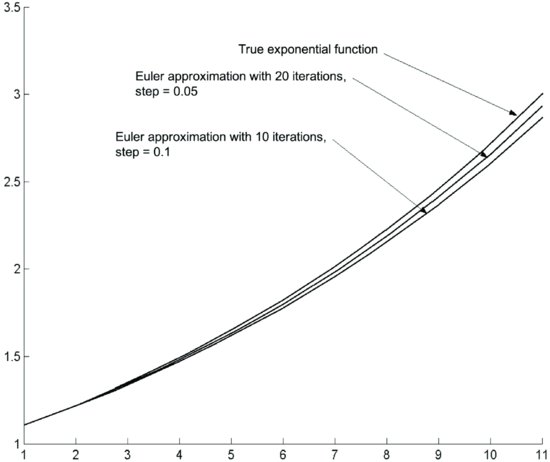
Suppose that we replace the derivative with its forward finite difference approximation and solve
If we assume that the step size is constant for all i:
![]()
The replacement of derivatives with finite differences is often called the Euler approximation. The differential equation is replaced by a recursive formula based on approximating the derivative with a finite difference. The i-th value of the solution is computed from the i−1-th value. Given the initial value of the function f, the solution of the differential equation can be arbitrarily approximated by choosing a sufficiently small interval. Figure 1 illustrates this computation for different values of Δx.
In the previous example of a first-order linear equation, only one initial condition was involved. Let’s now consider a second-order equation:
![]()
This equation describes oscillatory motion, such as the elongation of a pendulum or the displacement of a spring.
Figure 2 Numerical Solution of the Equation f ′′ + f = 0 with the Euler Approximation
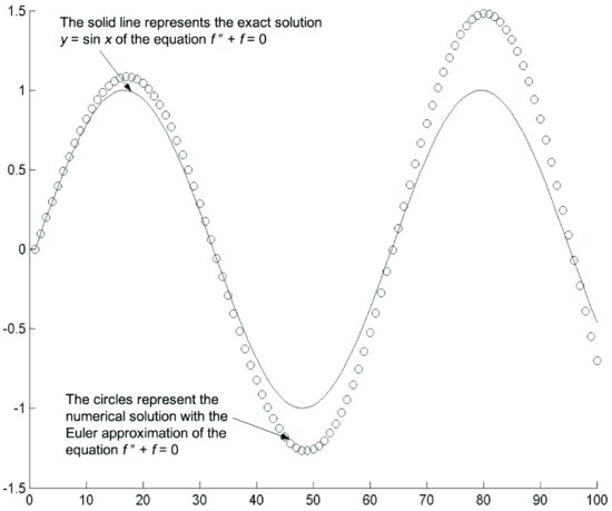
To approximate this equation we must approximate the second derivative. This could be done, for example, by combining difference quotients as follows:

With this approximation, the original equation becomes
We can thus write the approximation scheme:
![]()
Given the increment Δx and the initial values f(0), f′(0), using the above formulas we can recursively compute f(0 + Δx), f(0 + 2Δx), and so on. Figure 2 illustrates this computation.
Figure 3 Numerical Solution of the Equation f′ = f with the Runge-Kutta Method After 10 Steps
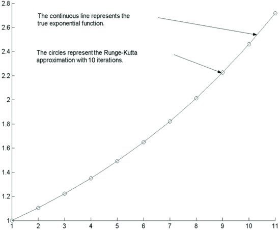
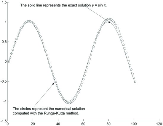
In practice, the Euler approximation scheme is often not sufficiently precise and more sophisticated approximation schemes are used. For example, a widely used approximation scheme is the Runge-Kutta method. We give an example of the Runge-Kutta method in the case of the equation f′′ + f = 0 which is equivalent to the linear system:
![]()
In this case the Runge-Kutta approximation scheme is the following:
Figures 3 and 4 illustrate the results of this method in the two cases f′ = f and f′′ + f = 0.
Figure 4 Numerical Solution of the Equation f′′ + f = 0 with the Runge-Kutta Method
As mentioned above, this numerical method depends critically on our having as givens (1) the initial values of the solution, and (2) its first derivative. Suppose that instead of initial values two boundary values were given, for instance the initial value of the solution and its value 1,000 steps ahead, that is, f(0) = f0, f(0 + 1,000Δx) = f1000. Conditions like these are rarely used in the study of dynamical systems as they imply foresight, that is, knowledge of the future position of a system. However, they often appear in static systems and when trying to determine what initial conditions should be imposed to reach a given goal at a given date.
In the case of boundary conditions, one cannot write a direct recursive scheme; it’s necessary to solve a system of equations. For instance, we could introduce the derivative f′(x) = δ as an unknown quantity. The difference quotient that approximates the derivative becomes an unknown. We can now write a system of linear equations in the following way:
This is a system of 1,000 equations in 1,000 unknowns. Solving the system we compute the entire solution. In this system two equations, the first and the last, are linked to boundary values; all other equations are transfer equations that express the dynamics (or the law) of the system. This is a general feature of boundary value problems. We will encounter it again when discussing numerical solutions of partial differential equations.
In the above example, we chose a forward scheme where the derivative is approximated with the forward difference quotient. One might use a different approximation scheme, computing the derivative in intervals centered around the point x. When derivatives of higher orders are involved, the choice of the approximation scheme becomes critical. Recall that when we approximated first and second derivatives using forward differences, we were required to evaluate the function at two points (i, i + 1) and three points (i,i + 1,i + 2) ahead respectively. If purely forward schemes are employed, computing higher-order derivatives requires many steps ahead. This fact might affect the precision and stability of numerical computations.
We saw in the examples that the accuracy of a finite difference scheme depends on the discretization interval. In general, a finite difference scheme works, that is, it is consistent and stable, if the numerical solution converges uniformly to the exact solution when the length of the discretization interval tends to zero. Suppose that the precision of an approximation scheme depends on the length of the discretization interval Δx. Consider the difference ![]() between the approximate and the exact solutions. We say that δf → 0 uniformly in the interval [a,b] when Δx→ 0 if, given any ε arbitrarily small, it is possible to find a Δx such that
between the approximate and the exact solutions. We say that δf → 0 uniformly in the interval [a,b] when Δx→ 0 if, given any ε arbitrarily small, it is possible to find a Δx such that ![]() .
.
NONLINEAR DYNAMICS AND CHAOS
Systems of differential equations describe dynamical systems that evolve starting from initial conditions. A fundamental concept in the theory of dynamical systems is that of the stability of solutions. This topic has become of paramount importance with the development of nonlinear dynamics and with the discovery of chaotic phenomena. We can only give a brief introductory account of this subject whose role in economics is still the subject of debate.
Intuitively, a dynamical system is considered stable if its solutions do not change much when the system is only slightly perturbed. There are different ways to perturb a system: changing parameters in its equations, changing the known functions of the system by a small amount, or changing the initial conditions.
Consider an equilibrium solution of a dynamical system, that is, a solution that is time invariant. If a stable system is perturbed when it is in a position of equilibrium, it tends to return to the equilibrium position or, in any case, not to diverge indefinitely from its equilibrium position. For example, a damped pendulum—if perturbed from a position of equilibrium—will tend to go back to an equilibrium position. If the pendulum is not damped it will continue to oscillate forever.
Consider a system of n equations of first order. (As noted above, systems of higher orders can always be reduced to first-order systems by enlarging the set of variables.) Suppose that we can write the system explicitly in the first derivatives as follows:
If the equations are all linear, a complete theory of stability has been developed. Essentially, linear dynamical systems are stable except possibly at singular points where solutions might diverge. In particular, a characteristic of linear systems is that they incur only small changes in the solution as a result of small changes in the initial conditions.
However, during the 1970s, it was discovered that nonlinear systems have a different behavior. Suppose that a nonlinear system has at least three degrees of freedom (that is, it has three independent nonlinear equations). The dynamics of such a system can then become chaotic in the sense that arbitrarily small changes in initial conditions might diverge. This sensitivity to initial conditions is one of the signatures of chaos. Note that while discrete systems such as discrete maps can exhibit chaos in one dimension, continuous systems require at least three degrees of freedom (that is, three equations).
Sensitive dependence from initial conditions was first observed in 1960 by the meteorologist Edward Lorenz of the Massachusetts Institute of Technology. Lorenz remarked that computer simulations of weather forecasts starting, apparently, from the same meteorological data could yield very different results. He argued that the numerical solutions of extremely sensitive differential equations such as those he was using produced diverging results due to rounding-off errors made by the computer system. His discovery was published in a meteorological journal where it remained unnoticed for many years.
Fractals
While in principle deterministic chaotic systems are unpredictable because of their sensitivity to initial conditions, the statistics of their behavior can be studied. Consider, for example, the chaos laws that describe the evolution of weather: While the weather is basically unpredictable over long periods of time, long-run simulations are used to predict the statistics of weather.
It was discovered that probability distributions originating from chaotic systems exhibit fat tails in the sense that very large, extreme events have nonnegligible probabilities. (See Brock, Hsieh, and LeBaron [1991] and Hsieh [1991].) It was also discovered that chaotic systems exhibit complex unexpected behavior. The motion of chaotic systems is often associated with self-similarity and fractal shapes.
Fractals were introduced in the 1960s by Benoit Mandelbrot, a mathematician working at the IBM research center in Yorktown Heights, New York. Starting from the empirical observation that cotton price time-series are similar at different time scales, Mandelbrot developed a powerful theory of fractal geometrical objects. Fractals are geometrical objects that are geometrically similar to part of themselves. Stock prices exhibit this property insofar as price time-series look the same at different time scales.
Chaotic systems are also sensitive to changes in their parameters. In a chaotic system, only some regions of the parameter space exhibit chaotic behavior. The change in behavior is ab-rupt and, in general, it cannot be predicted ana-lytically. In addition, chaotic behavior appears in systems that are apparently very simple.
While the intuition that chaotic systems might exist is not new, the systematic exploration of chaotic systems started only in the 1970s. The discovery of the existence of nonlinear chaotic systems marked a conceptual crisis in the physical sciences: It challenges the very notion of the applicability of mathematics to the description of reality. Chaos laws are not testable on a large scale; their applicability cannot be predicted analytically. Nevertheless, the statistics of chaos theory might still prove to be meaningful.
The economy being a complex system, the expectation was that its apparently random behavior could be explained as a deterministic chaotic system of low dimensionality. Despite the fact that tests to detect low-dimensional chaos in the economy have produced a substantially negative response, it is easy to make macroeconomic and financial econometric models exhibit chaos. (See Brock, Dechert, Scheinkman, and LeBaron [1996] and Brock and Hommes [1997].) As a matter of fact, most macroeconomic models are nonlinear. Though chaos has not been detected in economic time-series, most economic dynamic models are nonlinear in more than three dimensions and thus potentially chaotic. At this stage of the research, we might conclude that if chaos exists in economics it is not of the low-dimensional type.
PARTIAL DIFFERENTIAL EQUATIONS
To illustrate the notion of a partial differential equation (PDE), let’s start with equations in two dimensions. An n-order PDE in two dimensions x,y is an equation of the form
A solution of the previous equation will be any function that satisfies the equation.
In the case of PDEs, the notion of initial conditions must be replaced with the notion of boundary conditions or initial plus boundary conditions. Solutions will be defined in a multidimensional domain. To identify a solution uniquely, the value of the solution on some subdomain must be specified. In general, this subdomain will coincide with the boundary (or some portion of the boundary) of the domain.
Diffusion Equation
Different equations will require and admit different types of boundary and initial conditions. The question of the existence and uniqueness of solutions of PDEs is a delicate mathematical problem. We can only give a brief account by way of an example.
Let’s consider the diffusion equation. This equation describes the propagation of the probability density of stock prices under the random-walk hypothesis:
![]()
The Black-Scholes equation, which describes the evolution of option prices, can be reduced to the diffusion equation.
The diffusion equation describes propagating phenomena. Call f(t,x) the probability density that prices have value x at time t. In finance theory, the diffusion equation describes the time-evolution of the probability density function f(t,x) of stock prices that follow a random walk.2 It is therefore natural to impose initial and boundary conditions on the distribution of prices.
In general, we distinguish two different problems related to the diffusion equation: the first boundary value problem and the Cauchy initial value problem, named after the French mathematician Augustin Cauchy who first formulated it. The two problems refer to the same diffusion equation but consider different domains and different initial and boundary conditions. It can be demonstrated that both problems admit a unique solution.
The first boundary value problem seeks to find in the rectangle 0 ≤ x ≤ l, 0 ≤ t ≤ T a continuous function f(t,x) that satisfies the diffusion equation in the interior Q of the rectangle plus the following initial condition,
![]()
and boundary conditions,
![]()
The functions f1, f2 are assumed to be continuous and f1(0) = ϕ(0), f2(0) = ϕ(l).
The Cauchy problem is related to an infinite half plane instead of a finite rectangle. It is formulated as follows. The objective is to find for any x and for t ≥ 0 a continuous and bounded function f(t,x) that satisfies the diffusion equation and which, for t = 0, is equal to a continuous and bounded function ![]() .
.
Solution of the Diffusion Equation
The first boundary value problem of the diffusion equation can be solved exactly. We illustrate here a widely used method based on the separation of variables, which is applicable if the boundary conditions on the vertical sides vanish (that is, if f1(t) = f2(t) = 0). The method involves looking for a tentative solution in the form of a product of two functions, one that depends only on t and the other that depends only on x: f(t,x) = h(t)g(x).
If we substitute the previous tentative solution in the diffusion equation
![]()
we obtain an equation where the left side depends only on t while the right side depends only on x:
This condition can be satisfied only if the two sides are equal to a constant. The original diffusion equation is therefore transformed into two ordinary differential equations:
with boundary conditions g(0) = g(l) = 0. From the above equations and boundary conditions, it can be seen that b can assume only the negative values,
![]()
while the functions g can only be of the form
![]()
Substituting for h, we obtain
![]()
Therefore, we can see that there are denumerably infinite solutions of the diffusion equation of the form
![]()
All these solutions satisfy the boundary conditions f(t,0) = f(t,l) = 0. By linearity, we know that the infinite sum
will satisfy the diffusion equation. Clearly f(t,x) satisfies the boundary conditions f(t,0) = f(t,l) = 0. In order to satisfy the initial condition, given that ϕ(x) is bounded and continuous and that ϕ(0) = ϕ(l) = 0, it can be demonstrated that the coefficients Cs can be uniquely determined through the following integrals, which are called the Fourier integrals:
Figure 5 Solution of the Cauchy Problem by the Finite Difference Method
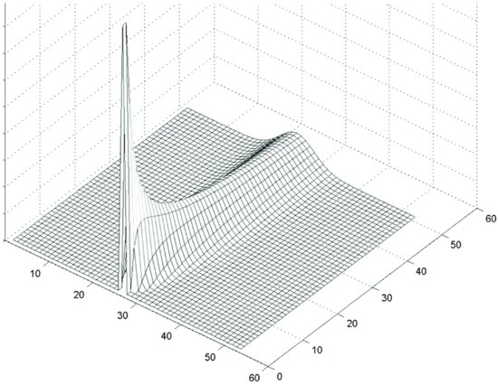
The previous method applies to the first boundary value problem but cannot be applied to the Cauchy problem, which admits only an initial condition. It can be demonstrated that the solution of the Cauchy problem can be expressed in terms of a convolution with a Green’s function. In particular, it can be demonstrated that the solution of the Cauchy problem can be written in closed form as follows:
for t > 0 and f(0,x) = ϕ(x). It can be demonstrated that the Black-Scholes equation, which is an equation of the form
![]()
can be reduced through transformation of variables to the standard diffusion equation to be solved with the Green’s function approach.
Numerical Solution of PDEs
There are different methods for the numerical solution of PDEs. We illustrate the finite difference methods, which are based on approximating derivatives with finite differences. Other discretization schemes such as finite elements and spectral methods are possible but, being more complex, they go beyond the scope of this book.
Finite difference methods result in a set of recursive equations when applied to initial conditions. When finite difference methods are applied to boundary problems, they require the solution of systems of simultaneous linear equations. PDEs might exhibit boundary conditions, initial conditions, or a mix of the two.
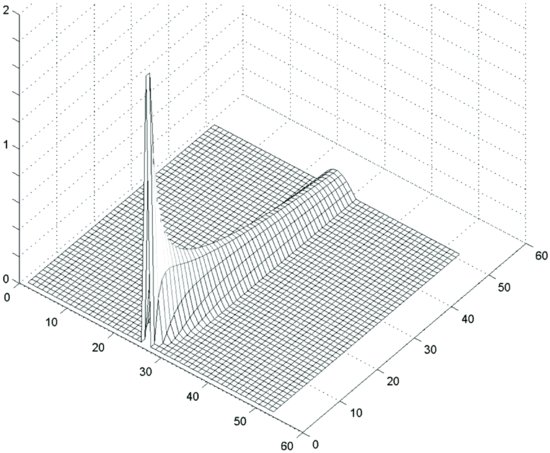
Figure 6 Solution of the First Boundary Problem by the Finite Difference Method
The Cauchy problem of the diffusion equation is an example of initial conditions. The simplest discretization scheme for the diffusion equation replaces derivatives with their difference quotients. As for ordinary differential equations, the discretization scheme can be written as follows:
In the case of the Cauchy problem, this approximation scheme defines the forward recursive algorithm. It can be proved that the algorithm is stable only if the Courant-Friedrichs-Lewy (CFL) conditions
![]()
are satisfied.
Different approximation schemes can be used. In particular, the forward approximation to the derivative used above could be replaced by centered approximations. Figure 5 illustrates the solution of a Cauchy problem for initial conditions that vanish outside of a finite interval. The simulation shows that solutions diffuse in the entire half space.
Applying the same discretization to a first boundary problem would require the solution of a system of linear equations at every step. Figure 6 illustrates this case.
KEY POINTS
- Basically, differential equations are equations that express a relationship between a function and one or more derivatives (or differentials) of that function.
- The two classifications of differential equations are ordinary differential equations and partial differential equations. The classification depends on the type of derivatives included in the differential equation: ordinary differential equation when there is only an ordinary derivative and partial differential equation where there are partial derivatives.
- Typically in differential equations, one of the independent variables is time.
- The term stochastic differential equation refers to a differential equation in which a derivative of one or more of the independent variables is a random variable or a stochastic process.
- Differential equations are conditions that must be satisfied by their solutions. Differential equations generally admit infinite solutions. Initial or boundary conditions are needed to identify solutions uniquely.
- Differential equations are the key mathematical tools for the development of modern science; in finance they are used in arbitrage pricing, to define stochastic processes, and to compute the time evolution of averages.
- Differential equations can be solved in closed form or with numerical methods. Finite difference methods approximate derivatives with difference quotients. Initial conditions yield recursive algorithms.
- Boundary conditions require the solution of linear equations.
NOTES
1. The condition of existence and continuity of derivatives is stronger than necessary. The Lipschitz condition, which requires that the incremental ratio be uniformly bounded in a given interval, would suffice.
2. In physics, the diffusion equation describes phenomena such as the diffusion of particles suspended in some fluid. In this case, the diffusion equation describes the density of particles at a given moment at a given point.
REFERENCES
Brock, W., Dechert, W. D., Scheinkman, J. A., and LeBaron, B. (1996). A test for independence based on the correlation dimension. Econometric Reviews 15, 3: 197–235.
Brock, W., and Hommes, C. (1997). A rational route to randomness. Econometrica 65, 5: 1059–1095.
Brock, W., Hsieh, D., and LeBaron, B. (1991). Nonlinear Dynamics, Chaos, and Instability. Cambridge, MA: MIT Press.
Hsieh, D. (1991). Chaos and nonlinear dynamics: Application to financial markets. Journal of Finance 46, 5: 1839–1877.
King, A. C., Billingham, J., and Otto, S. R. (2003). Differential Equations: Linear, Nonlinear, Ordinary, Partial. New York: Cambridge University Press.