
Important Functions and Their Features
In this entry, we review the functions that are used in financial modeling: continuous functions, the indicator function, the derivative of a function, monotonic functions, and the integral. Moreover, as special functions, we get to know the factorial, the gamma, beta, and Bessel functions as well as the characteristic function of random variables. (For a more detailed discussion of these functions, see Khuri [2003], MacCluer [2009], and Richardson [2008].)
CONTINUOUS FUNCTION
In this section, we introduce general continuous functions.
Figure 1 Continuous Function f(x)
Note: For x ∈ [0,1), f(x) = x2 and for x ∈ [1,2), f(x) = 1 + ln(x).
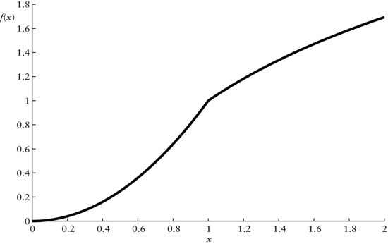
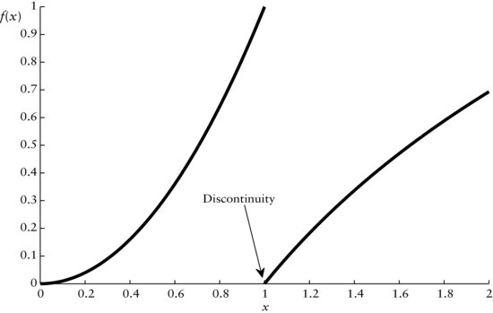
Figure 2 Discontinuous Function f(x)
Note: For x ∈ [0,1), f(x) = x2 and for x ∈ [1,2), f(x) = ln(x).
General Idea
Let f(x) be a continuous function for some real-valued variable x. The general idea behind continuity is that the graph of f(x) does not exhibit gaps. In other words, f(x) can be thought of as being seamless. We illustrate this in Figure 1. For increasing x, from x = 0 to x = 2, we can move along the graph of f(x) without ever having to jump. In the figure, the graph is generated by the two functions f(x) = x2 for x ∈ [0,1), and f(x) = ln(x) + 1 for x ∈ [1, 2).
Note that the function f(x) = ln (x) is the natural logarithm. It is the inverse function to the exponential function g(x) = ex where e = 2.7183 is the Euler constant. The inverse has the effect that f(g(x)) = ln(ex) = x, that is, ln and e cancel each other out.
A function f(x) is discontinuous if we have to jump when we move along the graph of the function. For example, consider the graph in Figure 2. Approaching x = 1 from the left, we have to jump from f(x) = 1 to f(1) = 0. Thus, the function f is discontinuous at x = 1. Here, f is given by f(x) = x2 for x ∈ [0,1), and f(x) = ln(x) for x ∈ [1,2).
Formal Derivation
For a formal treatment of continuity, we first concentrate on the behavior of f at a particular value x*.
We say that that a function f(x) is continuous at x* if, for any positive distance δ, we obtain a related distance ε(δ) such that
![]()
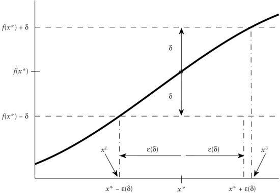
What does that mean? We use Figure 3 to illustrate. (The function is f(x) = sin(x) with x* = 0.2.) At x*, we have the value f(x*). Now, we select a neighborhood around f(x*) of some arbitrary distance δ as indicated by the dashed horizontal lines through f(x*) − δ and f(x*) + δ, respectively. From the intersections of these horizontal lines and the function graph (solid line), we extend two vertical dash-dotted lines down to the x-axis so that we obtain the two values xL and xU, respectively. Now, we measure the distance between xL and x* and also the distance between xU and x*. The smaller of the two yields the distance ε(δ). With this distance ε(δ) on the x-axis, we obtain the environment (x* − ε(δ), x* + ε(δ)) about x*. (Note that xL = x* − εδ, since the distance between xL and x* is the shorter one.) The environment is indicated by the dashed lines extending vertically above x* − ε(δ) and x* + ε(δ), respectively. We require that all x that lie in (x* − ε(δ), x* + ε(δ)) yield values f(x) inside of the environment [f(x*)−δ, f(x*) + δ]. We can see by Figure 3 that this is satisfied.
Let us repeat this procedure for a smaller distance δ. We obtain new environments [f(x*) − δ, f(x*) + δ] and (x* − ε(δ), x* + ε(δ)). If, for all x in (x* − ε(δ), x*+ ε(δ)), the f(x) are inside of [f(x*) − δ, f(x*) + δ], again, then we can take an even smaller δ. We continue this for successively smaller values of δ just short of becoming 0 or until the condition on the f(x) is no longer satisfied. As we can easily see in Figure 3, we could go on forever and the condition on the f(x) would always be satisfied. Hence, the graph of f is seamless or continuous at x.
Finally, we say that the function f is continuous if it is continuous at all x for which f is defined, that is, in the domain of f. Note that only the domain of f is of interest. For example, the square root function f(x) = ![]() is only defined for x ≥ 0. Thus, we do not care about whether f is continuous for any x other than x ≥ 0.
is only defined for x ≥ 0. Thus, we do not care about whether f is continuous for any x other than x ≥ 0.
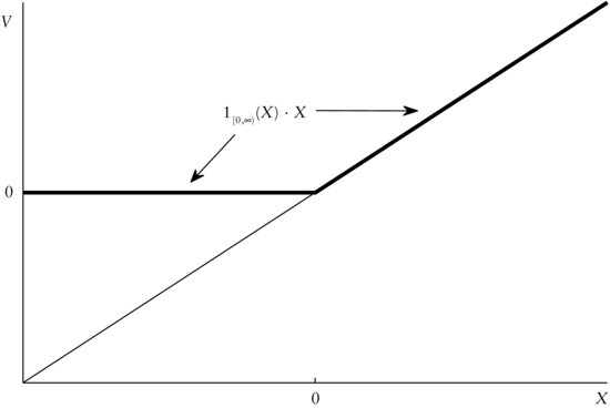
Figure 4 The Company Value V as a Function of the Random Variable X Using the Indicator Function 1[0,∞)(X) · X
INDICATOR FUNCTION
The indicator function acts like a switch. Often, it is denoted by 1A(X) where A is the event of interest and X is a random variable. So, 1A(X) is 1 if the event A is true, that is, if X assumes a value in A. Otherwise, 1A(X) is 0. Formally, this is expressed as
![]()
Usually, indicator functions are applied if we are interested in whether a certain event has occurred or not. For example, in a simple way, the value V of a company may be described by a real numbered random variable X on Ω = R with a particular probability distribution P. Now, the value V of the company may be equal to X as long as X is greater than 0. In the case where X assumes a negative value or 0, then V is automatically 0, that is, the company is bankrupt. So, the event of interest is A = [0, ∞), that is, we want to know whether X is still positive. Using the indicator function this can be expressed as
![]()
Finally, the company value can be given as
![]()
The company value V as a function is depicted in Figure 4. We can clearly detect the kink at x = 0 where the indicator function becomes 1 and, hence, V = X.
Figure 5 Function f (solid) with Derivatives f′(x) at x, for 0 < x < 0.5 (dashed), x = 1 (dash-dotted), and x = 1.571 (dotted)
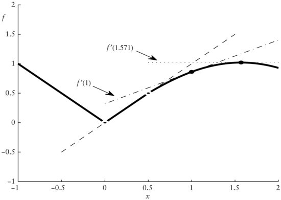
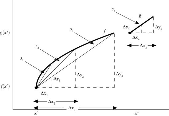
Figure 6 Functions f and g with Slopes Measured at the Points (x*, f(x*)) and (x+, g(x+)) Indicated by the • Symbol
DERIVATIVES
Suppose we have some continuous function f with the graph given by the solid line in Figure 5. We now might be interested in the growth rate of f at some position x. That is, we might want to know by how much f increases or decreases when we move from some x by a step of a given size, say Δx, to the right. This difference in f we denote by Δf. This Δ symbol is called delta.
Let us next have a look at the graphs given by the solid lines in Figure 6. These represent the graphs of f and g. The important difference between f and g is that, while g is linear, f is not, as can be seen by f′s curvature.
We begin the analysis of the graphs’ slopes with function g on the top right of the figure. Let us focus on the point (x+, g(x+)) given by the solid circle at the lower end of graph g. Now, when we move to the right by Δx4 along the horizontal dashed line, the corresponding increase in g is given by Δy4, as indicated by the vertical dashed line. If, on the other hand, we moved to the right by the longer distance, Δx5, the according increment of g would be given by Δy5. (This vertical increment Δy5 is also indicated by a vertical dashed line.) Since g is linear, it has constant slope everywhere and, hence, also at the point (x+, f(x+)). We denote that slope by s4. This implies that the ratios representing the relative increments (i.e., the slopes) have to be equal. That is,
![]()
Next, we focus on the graph of f on the lower left of Figure 6. Suppose we measured the slope of f at the point (x*, f(x*)). If we extended a step along the dashed line to the right by Δx1, the corresponding increment in f would be Δy1, as indicated by the leftmost vertical dashed line. If we moved, instead, by the longer Δx2 to the right, the corresponding increment in f would be Δy2. And a horizontal increment of Δx3 would result in an increase of f by Δy3.
In contrast to the graph of g, the graph of f does not exhibit the property of a constant increment Δy in f per unit step Δx to the right. That is, there is no constant slope of f, which results in the fact that the three ratios of the relative increase of f are different. To be precise, we have
![]()
as can be seen in Figure 6. So, the shorter our step Δx to the right, the steeper the slopes of the thin solid lines through (x*, f(x*)) and the corresponding points on the curve, (x*+Δx1, f(x*+Δx1)), (x*+Δx2, f(x*+Δx2)), and (x*+Δx2, f(x*+Δx2)), respectively. That means that, the smaller the increment Δx, the higher the relative increment Δy of f. So, finally, if we moved only a minuscule step to the right from (x*, f(x*)), we would obtain the steepest thin line and, consequently, the highest relative increase in f given by
By letting Δx approach 0, we obtain the marginal increment, in case the limit of (1) exists (i.e., if the ratio has a finite limit). Formally,
![]()
This marginal increment s(x) is different, at any point on the graph of f, while we have seen that it is constant for all points on the graph of g.
Construction of the Derivative
The limit analysis of marginal increments now brings us to the notion of a derivative that we discuss next. Earlier we introduced the limit growth rate of some continuous function at some point (x0, f(x0)). To represent the slope of the line through (x0, f(x0)) and (x0 + Δx, f(x0 + Δx)), we define the difference quotient
If we let Δx → 0, we obtain the limit of the difference quotient (2). If this limit is not finite, then we say that it does not exist. Suppose we were not only interested in the behavior of f when moving Δx to the right but also wanted to analyze the reaction by f to a step Δx to the left. We would then obtain two limits of (2). The first with Δx+ > 0 (i.e., a step to the right) would be the upper limit LU
![]()
and the second with Δx− < 0 (i.e., a step to the left), would be the lower limit LL
![]()
If LU and LL are equal, LU = LL = L, then f is said to be differentiable at x0. The limit L is the derivative of f. We commonly write the derivative in the fashion
On the right side of (3), we have replaced f(x) by the variable y as we will often do, for convenience. If the derivative (3) exists for all x, then f is said to be differentiable.
Let us now return to Figure 5. Recall that the graph of the continuous function fis given by the solid line. We start at x = −1. Since f is not continuous at x = −1, we omit this end point (1,1) from our analysis. For −1 < x < 0, we have that f is constant with slope s = −1. Consequently, the derivative f ′(x) = −1, for these x.
At x = 0, we observe that f is linear to the left with f′(x) = −1 and that it is also linear to the right, however, with f′(x) = 1, for 0 < x < 0.5. So, at x = 0, LU = 1 while LL = −1. Since here LU ≠ LL, the derivative of f does not exist at x = 0.
For 0 < x < 0.5, we have the constant derivative f′(x) = 1. The corresponding slope of 1 through (0,0) and (0.5,0.5) is indicated by the dashed line. At x = 0.5, the left side limit LL = 1 while the right side limit LU = 0.8776. (This value of cos(0.5) = 0.8776 is a result from calculus.) Hence, the two limits are not equal and, consequently, f is not differentiable at x = 0.5.
Without formal proof, we state that f is differentiable for all 0.5 < x < 2. For example, at x = 1, LL = LU = 0.5403 and, thus, the derivative f′(1) = 0.5403. The dash-dotted line indicating this derivative is called the tangent of f at x = 1. In Figure 5, the arrow indexed f′(1) points at this tangent. As another example, we select x = 1.571 where f assumes its maximum value. Here, the derivative f′(1.571) = 0 and, hence, the tangent at x = 1.571 is flat as indicated by the horizontal dotted line. In Figure 5, the arrow indexed f′ (1.571) points at this tangent.
MONOTONIC FUNCTION
Suppose we have some function f(x) for real-valued x. For example, the graph of f may look like that in Figure 7. We see that on the interval [0,1], the graph is increasing from f(0) = 0 to f(1) = 1. For 1 ≤ x ≤ 2, the graph remains at the level f(1) = 1 like a platform. And, finally, between x = 2 and x = 3, the graph is increasing, again, from f(2) = 1 to f(3) = 2.
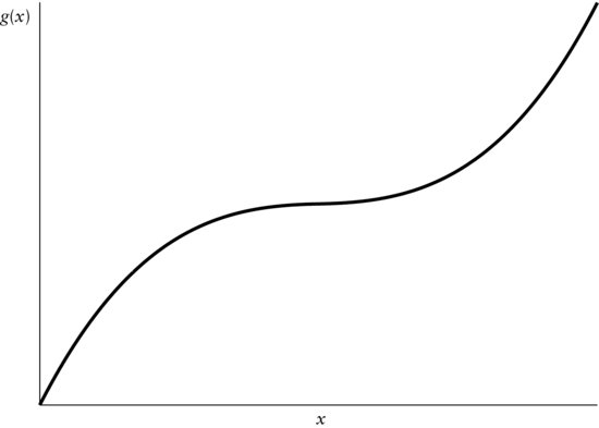
In contrast, we may have another function, g(x). Its graph is given by Figure 8. It looks somewhat similar to the graph in Figure 7, however, without the platform. The graph of g never remains at a level, but increases constantly. Even for the smallest increments from one value of x, say x1, to the next higher, say x2, there is always an upward slope in the graph.
Both functions, f and g, never decrease. The distinction is that f is monotonically increasing since the graph can remain at some level, while g is strictly monotonic increasing since its graph never remains at any level. If we can differentiate f and g, we can express this in terms of the derivatives of f and g. Let f′ be the derivative of f and g′ the derivative of g. Then, we have the following definitions of continuity for continuous functions with existing derivatives:
Monotonically increasing functions: A continuous function f with derivative f ′ is monotonically increasing if its derivative f ′ ≥ 0.
Strictly monotonic increasing functions: A continuous function g with derivative g′ is strictly monotonic increasing if its derivative g′ > 0.
Analogously, a function f(x) is monotonically decreasing if it behaves in the opposite manner. That is, f never increases when moving from some x to any higher value x1 > x. When f is continuous with derivative f′, then we say that f is monotonically decreasing if f′(x) ≤ 0 and that it is strictly monotonic increasing if f′(x) < 0 for all x. For these two cases, illustrations are given by mirroring the graphs in Figures 7 and 8 against their vertical axes, respectively.
Figure 7 Monotonically Increasing Function f
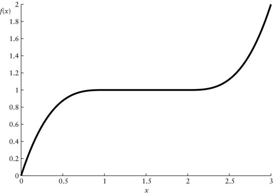
Figure 8 Strictly Monotonic Increasing Function g
INTEGRAL
Here we derive the concept of integration necessary to understand the probability density and continuous distribution function. The integral of some function over some set of values represents the area between the function values and the horizontal axis. To sketch the idea, we start with an intuitive graphical illustration.
We begin by analyzing the area A between the graph (solid line) of the function f(t) and the horizontal axis between t = 0 and t = T in Figure 9. Looking at the graph, it appears quite complicated to compute this area A in comparison to, for example, the area of a rectangle where we would only need to know its width and length. However, we can approximate this area by rectangles as will be done next.
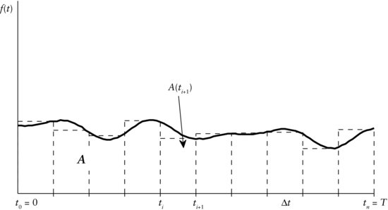
Figure 9 Approximation of the Area A between Graph of f(t) and the Horizontal Axis, for 0 ≤ t ≤ T
Approximation of the Area through Rectangles
Let’s approximate the area A under the function graph in Figure 9 as follows. As a first step, we dissect the interval between 0 and T into n equidistant intervals of length Δt = ti+1 − ti for i = 0, 1, … , n − 1. For each such interval, we consider the function value f(ti+1) at the rightmost point, ti+1. To obtain an estimate of the area under the graph for the respective interval, we multiply the value f(ti+1) at ti+1 by the interval width Δt yielding A (ti+1) = Δt · f (ti+1), which equals the area of the rectangle above interval i + 1 as displayed in Figure 9. Finally, we add up the areas A(t1), A(t2), … , A(T) of all rectangles resulting in the desired estimate of the area A
We repeat the just described procedure for decreasing interval widths Δt.
Integral as the Limiting Area
To derive the perfect approximation of the area under the curve in Figure 9, we let the interval width Δt gradually vanish until it almost equals 0, proceeding as before. We denote this infinitesimally small width by the step rate dt. Now, the difference between the function values at either end, that is, f(ti) and f(ti+1), of the interval i + 1 will be nearly indistinguishable since ti and ti+1 almost coincide. Hence, the corresponding rectangle with area A(ti+1) will turn into a dash with infinitesimally small base dt.
Summation as in equation (4) of the areas of the dashes becomes infeasible. For this purpose, the integral has been introduced as the limit of (4) as Δt → 0. (Conditions under which these limits exist are omitted here.) It is denoted by

where the limits 0 and T indicate which interval the integration is performed on. In our case, the integration variable is t while the function f(t) is called the integrand. In words, equation (5) is the integral of the function f(t) over t from 0 to T. It is immaterial how we denote the integration variable. The same result as in equation (5) would result if we wrote

instead. The important factors are the integrand and the integral limits.
Note that instead of using the function values of the right boundaries of the intervals f(ti+1) in equation (4), referred to as the right-point rule, we might as well have taken the function values of the left boundaries f(ti), referred to as the left-point rule, which would have led to the same integral. Moreover, we might have taken the function f(0.5·(ti+1 + ti)) values evaluated at the mid-points of the intervals and still obtained the same interval. This latter procedure is called the mid-point rule.
If we keep 0 as the lower limit of the integral in equation (5) and vary T, then equation (5) becomes a function of the variable T. We may denote this function by
Relationship Between Integral and Derivative
In equation (6) the relationship between f(t) and F(T) is as follows. Suppose we compute the derivative of F(T) with respect to T and assume that F(T) is differentiable, for T > 0. The result is
Hence, from equation (7) we see that the marginal increment of the integral at any point (i.e., its derivative) is exactly equal to the integrand evaluated at the according value. This need not generally be true. But in most cases, particularly in financial modeling, this statement is valid.
The implication of this discussion for probability theory is as follows. Let P be a continuous probability measure with probability distribution function F and (probability) density function f. There is the unique link between f and P given through
Formally, the integration of f over x is always from −∞ to ∞, even if the support is not on the entire real line. This is no problem, however, since the density is zero outside the support and, hence, integration over those parts yields 0 contribution to the integral. For example, suppose that some density function were
where h(x) is just some function such that f satisfies the requirements for a density function. That is, the support is only on the positive part of the real line. Substituting the function from equation (9) into equation (8) yields the equality
(10) 
SOME FUNCTIONS
Here we introduce some functions needed in probability theory to describe probability distributions of random variables: factorials, gamma function, beta function, Bessel function of the third kind, and characteristic function. While the first four are functions of very special shape, the characteristic function is of a more general structure. It is the function characterizing the probability distribution of some random variable and, hence, is of unique form for each random variable.
Factorial
Let k ∈ N (i.e., k = 1, 2, …). Then the factorial of this natural number k, denoted by the symbol !, is given by
A factorial is the product of this number and all natural numbers smaller than k including 1. By definition, the factorial of zero is one (i.e., 0! ≡ 1). For example, the factorial of 3 is 3! = 3 · 2 · 1 = 6.
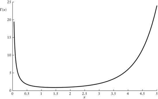
Figure 10 Gamma Function Γ(x)
Gamma Function
The gamma function for nonnegative values x is defined by
The gamma function has the following properties. If the x correspond with a natural number n ∈ N (i.e., n = 1, 2, …), then we have that equation (12) equals the factorial given by equation (11) of n − 1. Formally, this is
![]()
Furthermore, for any x ≥ 0, it holds that Γ(x +1) = xΓ(x).
In Figure 10, we have displayed part of the gamma function for x values between 0.1 and 5. Note that, for either x → 0 or x → ∞, Γ(x) goes to infinity.
Beta Function
The beta function with parameters c and d is defined as
where Γ is the gamma function from equation (12).
Bessel Function of the Third Kind
The Bessel function of the third kind is defined as
This function is often a component of other, more complex functions such as the density function of the NIG distribution.
Characteristic Function
Before advancing to introduce the characteristic function, we briefly explain complex numbers.
Suppose we were to take the square root of the number −1, that is, ![]() . So far, our calculus has no solution for this since the square root of negative numbers has not yet been introduced. However, by introducing the imaginary number i, which is defined as
. So far, our calculus has no solution for this since the square root of negative numbers has not yet been introduced. However, by introducing the imaginary number i, which is defined as
Figure 11 Graphical Representation of the Complex Number z = 0.8 + 0.9i

![]()
we can solve square roots of any real number. Now, we can represent any number as the combination of a real (Re) part a plus some units b of i, which we refer to as the imaginary (Im) part. Then, any number z will look like
The number given by equation (13) is a complex number. The set of complex numbers is symbolized by C. This set contains the real numbers that are those complex numbers with b = 0. Graphically, we can represent the complex numbers on a two-dimensional space as given in Figure 11.
Now, we can introduce the characteristic function as some function ![]() mapping real numbers into the complex numbers. Formally, we write this as
mapping real numbers into the complex numbers. Formally, we write this as ![]() : R → C. Suppose we have some random variable X with density function f. The characteristic function is then defined as
: R → C. Suppose we have some random variable X with density function f. The characteristic function is then defined as
which transforms the density f into some complex number at any real position t. Equation (14) is commonly referred to as the Fourier transformation of the density.
The relationship between the characteristic function φ and the density function f of some random variable is unique. So, when we state either one, the probability distribution of the corresponding random variable is unmistakably determined.
KEY POINTS
- Continuous functions are an integral component of mathematical analysis. They are useful whenever jumps in the function values are undesirable. This is often the case when financial asset returns are modeled; that is, one assumes that, in particular logarithmic returns, they may assume any value on the real line such that the related probability distribution is continuous with continuous probability density.
- The indicator function is defined as a function yielding one for certain specified argument values and zero in any other case. It is helpful in expressing so-called exclusive either-or behavior of random variables (i.e., when random variables can only assume exactly one of two values). For example, when one models call option prices where, at maturity, the value of the option is equal to either zero or the difference between the market value of the underlying and the strike price, one resorts to the indicator function.
- The derivative of some function expresses the function’s rate of growth at some point for infinitesimally small increments. In words, it expresses by how much the function changes if one takes a very small step. In probability theory, a derivative is used in the context of a continuous probability distribution to express by how much the distribution function increases at a certain value (i.e., the marginal rate of probability at a certain value).
- The integral is the continuous analogue of the sum of discrete values. In probability theory, the probability of individual outcomes is always zero when the distribution is continuous. In order to express the probability of at most a certain value, we cannot sum the individual probabilities of all values less than or equal to the critical value. Instead, at each value, we have the density function which we integrate up to the critical value, yielding the requested probability.
- The characteristic function is the unique representation of a probability distribution. For certain distributions, the probability density function or the distribution function are unknown. Instead, it is necessary to resort to the characteristic function. Technically, the characteristic function is a function involving complex numbers (i.e., numbers including the square root of minus one) to express the behavior of some function at certain frequencies. It is closely linked to the Fourier transform used in engineering.
REFERENCES
Khuri, A. (2003). Advanced Calculus with Applications in Statistics, 2nd ed. Hoboken, NJ: John Wiley & Sons.
MacCluer, B. D. (2009). Elementary Functional Analysis. New York: Springer.
Richardson, L. F. (2008). Advanced Calculus: An Introduction to Linear Analysis. Hoboken, NJ: John Wiley & Sons.