
Nonlinearity and Nonlinear Econometric Models in Finance
In this entry, we study nonlinearity in financial data, discuss various nonlinear models available in the literature, and demonstrate application of nonlinear models in finance with real examples. The models discussed include bilinear models, threshold autoregressive models, smooth threshold autoregressive models, Markov switching models, and nonlinear additive autoregressive models. We also consider nonparametric methods and neural networks, and apply nonparametric methods to estimate interest models. To detect nonlinearity in financial data, we introduce various nonlinearity tests available in the literature and apply the tests to some financial series. Finally, we analyze the monthly U.S. unemployment rate and compare out-of-sample prediction of nonlinear models with linear ones via several criteria.
STUDY OF NONLINEARITY IN ECONOMETRICS AND STATISTICS
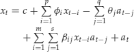
Assume, for simplicity, a univariate time series xt is observed at equally spaced time points. We denote the observations by {xt|t = 1, … , T}, where T is the sample size. A purely stochastic time series xt is said to be linear if it can be written as
where μ is a constant, ψi are real numbers with ψ0 = 1, and {at} is a sequence of independent and identically distributed (IID) random variables with a well-defined distribution function. We assume that the distribution of at is continuous and E(at) = 0. In many cases, we further assume that Var(at) = σ2a or, even stronger, that at is Gaussian. If ![]() , then Xt is weakly stationary (i.e., the first two moments of xt are time-invariant). The well-known autoregressive moving-average (ARMA) process of Box et al. (2008) is linear because it has an moving-average (MA) representation in equation (1). Any stochastic process that does not satisfy the condition of equation (1) is said to be nonlinear. The prior definition of nonlinearity is for purely stochastic time series. One may extend the definition by allowing the mean of xt to be a linear function of some exogenous variables, including the time index and some periodic functions. But such a mean function can be handled easily by using a regression model with time series errors discussed in Tsay (2010, Chapter 2), and we shall not consider the extension here. Mathematically, a purely stochastic time series model for xt is a function of an IID sequence consisting of the current and past shocks—that is,
, then Xt is weakly stationary (i.e., the first two moments of xt are time-invariant). The well-known autoregressive moving-average (ARMA) process of Box et al. (2008) is linear because it has an moving-average (MA) representation in equation (1). Any stochastic process that does not satisfy the condition of equation (1) is said to be nonlinear. The prior definition of nonlinearity is for purely stochastic time series. One may extend the definition by allowing the mean of xt to be a linear function of some exogenous variables, including the time index and some periodic functions. But such a mean function can be handled easily by using a regression model with time series errors discussed in Tsay (2010, Chapter 2), and we shall not consider the extension here. Mathematically, a purely stochastic time series model for xt is a function of an IID sequence consisting of the current and past shocks—that is,
The linear model in equation (1) says that f(.) is a linear function of its arguments. Any nonlinearity in f(.) results in a nonlinear model. The general nonlinear model in equation (2) is too vague to be useful in practice. Further assumptions are needed to make the model applicable.
To put nonlinear models available in the literature in a proper perspective, we write the model of xt in terms of its conditional moments. Let Ft−1 be the σ-field generated by available information at time t − 1 (inclusive). Typically, Ft−1 denotes the collection of linear combinations of elements in {xt−1, xt−2, …} and {at−1, at−2, …}. The conditional mean and variance of xt given Ft−1 are
where g(.) and h(.) are well-defined functions with h(.) > 0. Thus, we restrict the model to
![]()
where et = at/σt is a standardized shock (or innovation). For the linear series xt in equation (1), g(.) is a linear function of elements of Ft−1 and h(.) = σ2a. The development of nonlinear models involves making extensions of the two equations in equation (3). If g(.) is nonlinear, xt is said to be nonlinear in mean. If h(.) is time-variant, then xt is nonlinear in variance. The conditional heteroscedastic models, for example, the GARCH model of Bollerslev (1986), are nonlinear in variance because their conditional variances σ2t evolve over time. Based on the well-known Wold decomposition, a weakly stationary and purely stochastic time series can be expressed as a linear function of uncorrelated shocks. For stationary volatility series, these shocks are uncorrelated, but dependent. The models discussed in this entry represent another extension to nonlinearity derived from modifying the conditional mean equation in equation (3).
Many nonlinear time series models have been proposed in the statistical literature, such as the bilinear models of Granger and Andersen (1978), the threshold autoregressive (TAR) model of Tong (1978), the state-dependent model of Priestley (1980), and the Markov switching model of Hamilton (1989). The basic idea underlying these nonlinear models is to let the conditional mean μt evolve over time according to some simple parametric nonlinear function. Recently, a number of nonlinear models have been proposed by making use of advances in computing facilities and computational methods. Examples of such extensions include the nonlinear state-space modeling of Carlin, Polson, and Stoffer (1992), the functional-coefficient autoregressive model of Chen and Tsay (1993a), the nonlinear additive autoregressive model of Chen and Tsay (1993b), the multivariate adaptive regression spline of Lewis and Stevens (1991), and the generalized autoregressive score (GAS) model of Creal et al. (2010). The basic idea of these extensions is either using simulation methods to describe the evolution of the conditional distribution of xt or using data-driven methods to explore the nonlinear characteristics of a series. Finally, nonparametric and semiparametric methods such as kernel regression and artificial neural networks have also been applied to explore the nonlinearity in a time series. We discuss some nonlinear models in this entry that are applicable to financial time series. The discussion includes some nonparametric and semiparametric methods.
Apart from the development of various nonlinear models, there is substantial interest in studying test statistics that can discriminate linear series from nonlinear ones. Both parametric and nonparametric tests are available. Most parametric tests employ either the Lagrange multiplier or likelihood ratio statistics. Nonparametric tests depend on either higher order spectra of xt or the concept of dimension correlation developed for chaotic time series. We review some nonlinearity tests, discuss modeling and forecasting of nonlinear models, and provide an application of nonlinear models.
NONLINEAR MODELS
Most nonlinear models developed in the statistical literature focus on the conditional mean equation in equation (3); see Priestley (1988) and Tong (1990) for summaries of nonlinear models. Our goal here is to introduce some nonlinear models that are useful in finance.
Bilinear Model
The linear model in equation (1) is simply the first-order Taylor series expansion of the f(.) function in equation (2). As such, a natural extension to nonlinearity is to employ the second-order terms in the expansion to improve the approximation. This is the basic idea of bilinear models, which can be defined as
where p, q, m, and s are nonnegative integers. This model was introduced by Granger and Andersen (1978) and has been widely investigated. Subba Rao and Gabr (1984) discuss some properties and applications of the model, and Liu and Brockwell (1988) study general bilinear models. Properties of bilinear models such as stationarity conditions are often derived by (a) putting the model in a state-space form and (b) using the state transition equation to express the state as a product of past innovations and random coefficient vectors. A special generalization of the bilinear model in equation (4) has conditional heteroscedasticity. For example, consider the model
(5) ![]()
where {at} is a white noise series. The first two conditional moments of xt are

which confirm that the model has time-varying volatility.
Example 1. Consider the monthly simple returns of the CRSP equal-weighted index from January 1926 to December 2008 for 996 observations. Denote the series by Rt. The sample partial autocorrelation function (PACF) of Rt shows significant serial correlations at lags 1 and 3 so that an AR(3) model is used for the mean equation. The squared series of the AR(3) residuals suggests that the conditional heteroscedasticity might depend on lags 1, 3 and 8 of the residuals. Therefore, we employ the special bilinear model
![]()
for the series, where at = β0![]() with
with ![]() being an IID series with mean zero and variance 1. Note that lag 8 is omitted for simplicity. Assuming that the conditional distribution of at is normal, we use the conditional maximum likelihood method and obtain the fitted model
being an IID series with mean zero and variance 1. Note that lag 8 is omitted for simplicity. Assuming that the conditional distribution of at is normal, we use the conditional maximum likelihood method and obtain the fitted model
where the standard errors of the parameters are, in the order of appearance, 0.0023, 0.032, 0.027, 0.002, 0.147, and 0.136, respectively. All estimates are significantly different from zero at the 5% level. Define
![]()
where ![]() =0 for t ≤ 3 as the standardized residual series of the model. The sample autocorrelation function (ACF) of
=0 for t ≤ 3 as the standardized residual series of the model. The sample autocorrelation function (ACF) of ![]() shows no significant serial correlations, but the series is not independent because the squared series
shows no significant serial correlations, but the series is not independent because the squared series ![]() 2 has significant serial correlations. The validity of model (6) deserves further investigation. For comparison, we also consider an AR(3)-ARCH(3) model for the series and obtain
2 has significant serial correlations. The validity of model (6) deserves further investigation. For comparison, we also consider an AR(3)-ARCH(3) model for the series and obtain
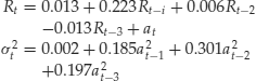
where all estimates but the coefficients of Rt−2 and Rt−3 are highly significant. The standardized residual series of the model shows no serial correlations, but the squared residuals show Q(10) = 19.78 with a p-value of 0.031. Models (6) and (7) appear to be similar, but the latter seems to fit the data better. Further study shows that an AR(1)-GARCH(1,1) model fits the data well.
Threshold Autoregressive (TAR) Model
This model is motivated by several nonlinear characteristics commonly observed in practice such as asymmetry in declining and rising patterns of a process. It uses piecewise linear models to obtain a better approximation of the conditional mean equation. However, in contrast to the traditional piecewise linear model that allows for model changes to occur in the “time” space, the TAR model uses threshold space to improve linear approximation. Let us start with a simple 2-regime AR(1) model
where the at are IID N(0,1). Here the threshold variable is xt−1 and the threshold is 0.
Figure 1 shows the time plot of a simulated series of xt with 200 observations. A horizontal line of zero is added to the plot, which illustrates several characteristics of TAR models. First, despite the coefficient −1.5 in the first regime, the process xt is geometrically ergodic and stationary. In fact, the necessary and sufficient condition for model (8) to be geometrically ergodic is ![]() < 1,
< 1, ![]() < 1 and
< 1 and ![]()
![]() <1, where
<1, where ![]() is the AR coefficient of regime i; see Petruccelli and Woolford (1984) and Chen and Tsay (1991).
is the AR coefficient of regime i; see Petruccelli and Woolford (1984) and Chen and Tsay (1991).
Figure 1 Time Plot of a Simulated 2-Regime TAR(1) Series
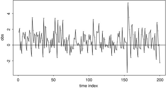
Ergodicity is an important concept in time series analysis. For example, the statistical theory showing that the sample mean![]() of xt converges to the mean of xt is referred to as the ergodic theorem, which can be regarded as the counterpart of the central limit theory for the IID case. Second, the series exhibits an asymmetric increasing and decreasing pattern. If xt−1 is negative, then xt tends to switch to a positive value due to the negative and explosive coefficient −1.5. Yet when xt−1 is positive, it tends to take multiple time periods for xt to reduce to a negative value. Consequently, the time plot of xt shows that regime 2 has more observations than regime 1, and the series contains large upward jumps when it becomes negative. The series is therefore not time-reversible. Third, the model contains no constant terms, but E(xt) is not zero. The sample mean of the particular realization is 0.61 with a standard deviation of 0.07. In general, E(xt) is a weighted average of the conditional means of the two regimes, which are nonzero. The weight for each regime is simply the probability that xt is in that regime under its stationary distribution. It is also clear from the discussion that, for a TAR model to have zero mean, nonzero constant terms in some of the regimes are needed. This is very different from a stationary linear model for which a nonzero constant implies that the mean of xt is not zero.
of xt converges to the mean of xt is referred to as the ergodic theorem, which can be regarded as the counterpart of the central limit theory for the IID case. Second, the series exhibits an asymmetric increasing and decreasing pattern. If xt−1 is negative, then xt tends to switch to a positive value due to the negative and explosive coefficient −1.5. Yet when xt−1 is positive, it tends to take multiple time periods for xt to reduce to a negative value. Consequently, the time plot of xt shows that regime 2 has more observations than regime 1, and the series contains large upward jumps when it becomes negative. The series is therefore not time-reversible. Third, the model contains no constant terms, but E(xt) is not zero. The sample mean of the particular realization is 0.61 with a standard deviation of 0.07. In general, E(xt) is a weighted average of the conditional means of the two regimes, which are nonzero. The weight for each regime is simply the probability that xt is in that regime under its stationary distribution. It is also clear from the discussion that, for a TAR model to have zero mean, nonzero constant terms in some of the regimes are needed. This is very different from a stationary linear model for which a nonzero constant implies that the mean of xt is not zero.
A time series xt is said to follow a k-regime self-exciting TAR (SETAR) model with threshold variable xt−d if it satisfies
where k and d are positive integers, j = 1, … , k, γi are real numbers such that -∞ = γ0 < γ1 < ... < γk-1 < γk = ∞, the superscript (j) is used to signify the regime, and {a(j)t} are IID sequences with mean 0 and variance σ2j and are mutually independent for different j. The parameter d is referred to as the delay parameter and γj are the thresholds. Here it is understood that the AR models are different for different regimes; otherwise, the number of regimes can be reduced. Equation (9) says that a SETAR model is a piecewise linear AR model in the threshold space. It is similar in spirit to the usual piecewise linear models in regression analysis, where model changes occur in the order in which observations are taken. The SETAR model is nonlinear provided that k > 1.
Properties of general SETAR models are hard to obtain, but some of them can be found in Tong (1990), Chan (1993), Chan and Tsay (1998), and the references therein. In recent years, there is increasing interest in TAR models and their applications; see, for instance, Hansen (1997), Tsay (1998), and Montgomery et al. (1998). Tsay (1989) proposed a testing and modeling procedure for univariate SETAR models. The model in equation (9) can be generalized by using a threshold variable zt that is measurable with respect to Ft−1 (i.e., a function of elements of Ft−1). The main requirements are that zt is stationary with a continuous distribution function over a compact subset of the real line and that zt−d is known at time t. Such a generalized model is referred to as an open-loop TAR model.
Example 2. To demonstrate the application of TAR models, consider the U.S. monthly civilian unemployment rate, seasonally adjusted and measured in percentage, from January 1948 to March 2009 for 735 observations. The data are obtained from the Bureau of Labor Statistics, Department of Labor, and are shown in Figure 2. The plot shows two main characteristics of the data. First, there appears to be a slow but upward trend in the overall unemployment rate. Second, the unemployment rate tends to increase rapidly and decrease slowly. Thus, the series is not time-reversible and may not be unit-root stationary, either.
Figure 2 Time Plot of Monthly U.S. Civilian Unemployment Rate, Seasonally Adjusted, from January 1948 to March 2009

Because the sample autocorrelation function decays slowly, we employ the first differenced series yt = (1−B)ut in the analysis, where ut is the monthly unemployment rate. Using univariate ARIMA models, we obtain the model
where ![]() = 0.187 and all estimates but the AR(2) coefficient are statistically significant at the 5% level. The t-ratio of the estimate of AR(2) coefficient is −1.66. The residuals of model (10) give Q(12) = 12.3 and Q(24) = 25.5, respectively. The corresponding p-values are 0.056 and 0.11, respectively, based on χ2 distributions with 6 and 18 degrees of freedom. Thus, the fitted model adequately describes the serial dependence of the data. Note that the seasonal AR and MA coefficients are highly significant with standard error 0.049 and 0.035, respectively, even though the data were seasonally adjusted. The adequacy of seasonal adjustment deserves further study. Using model (10), we obtain the 1-step ahead forecast of 8.8 for the April 2009 unemployment rate, which is close to the actual data of 8.9.
= 0.187 and all estimates but the AR(2) coefficient are statistically significant at the 5% level. The t-ratio of the estimate of AR(2) coefficient is −1.66. The residuals of model (10) give Q(12) = 12.3 and Q(24) = 25.5, respectively. The corresponding p-values are 0.056 and 0.11, respectively, based on χ2 distributions with 6 and 18 degrees of freedom. Thus, the fitted model adequately describes the serial dependence of the data. Note that the seasonal AR and MA coefficients are highly significant with standard error 0.049 and 0.035, respectively, even though the data were seasonally adjusted. The adequacy of seasonal adjustment deserves further study. Using model (10), we obtain the 1-step ahead forecast of 8.8 for the April 2009 unemployment rate, which is close to the actual data of 8.9.
To model nonlinearity in the data, we employ TAR models and obtain the model
where the standard errors of ait are 0.180 and 0.217, respectively, the standard errors of the AR parameters in regime 1 are 0.046, 0.043, 0.042, and 0.037 whereas those of the AR parameters in regime 2 are 0.054, 0.057, and 0.075, respectively. The number of data points in regimes 1 and 2 are 460 and 262, respectively. The standardized residuals of model (11) only shows some minor serial correlation at lag 12. Based on the fitted TAR model, the dynamic dependence in the data appears to be stronger when the change in monthly unemployent rate is greater than 0.1%. This is understandable because a substantial increase in the unemployment rate is indicative of weakening in the U.S. economy, and policy makers might be more inclined to take action to help the economy, which in turn may affect the dynamics of the unemployment rate series. Consequently, model (11) is capable of describing the time-varying dynamics of the U.S. unemployment rate.
The MA representation of model (10) is
![]()
It is then not surprising to see that no yt−1 term appears in model (11).
Threshold models can be used in finance to handle the leverage effect, that is, volatility responds differently to prior positive and negative returns. The models can also be used to study arbitrage trading in index futures and cash prices. See Tsay (2010, chap. 8) for discussions and demonstration. Here we focus on volatility modeling and introduce an alternative approach to parameterization of threshold GARCH (TGARCH) models. In some applications, this new general TGARCH model fares better than the model of Glosten et al. (1993).
Example 3. Consider the daily log returns, in percentages and including dividends, of IBM stock from January 2, 2001 to December 31, 2009 for 2,263 observations. Figure 3 shows the time plot of the series. The volatility seems to be larger at the beginning and end of the data span. If GARCH models are entertained, we obtain the following GARCH(1,1) model for the series:
Figure 3 Time Plot of the Daily Log Returns, in Percentages, for IBM Stock from January 2, 2001 to December 31, 2009
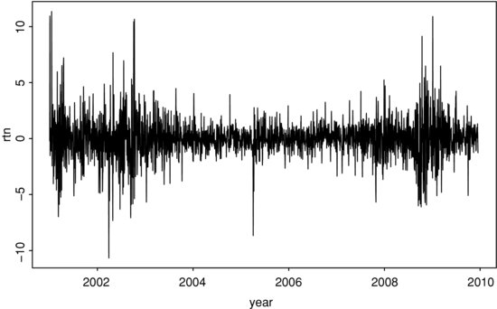
where rt is the log return, {et} is a Gaussian white noise sequence with mean zero and variance 1.0, the standard error of the constant term in the mean equation is 0.026, and those of the volatility equation are 0.012, 0.020, and 0.021, respectively. All estimates are statistically significant at the 5% level. The Ljung-Box statistics of the standardized residuals, ![]() give Q(10) = 10.08(0.43) and Q(20) = 23.24(0.28), where the number in parentheses denotes p-value obtained using the asymptotic X2m distribution. For the squared standardized residuals, we obtain Q(10) = 7.38(0.69) and Q(20) = 15.43(0.75). The model is adequate in modeling the serial dependence and conditional heteroscedasticity of the data. But the unconditional mean for rt of model (12) is 0.058, which is substantially larger than the sample mean 0.024, indicating that the model might be misspecified.
give Q(10) = 10.08(0.43) and Q(20) = 23.24(0.28), where the number in parentheses denotes p-value obtained using the asymptotic X2m distribution. For the squared standardized residuals, we obtain Q(10) = 7.38(0.69) and Q(20) = 15.43(0.75). The model is adequate in modeling the serial dependence and conditional heteroscedasticity of the data. But the unconditional mean for rt of model (12) is 0.058, which is substantially larger than the sample mean 0.024, indicating that the model might be misspecified.
Next, we employ the TGARCH model of Glosten et al. (1993) and obtain
where Nt−1 is the indicator for negative at−1 such that Nt−1 = 1 if at−1 < 0 and = 0 otherwise, the standard error of the parameter in the mean equation is 0.026, and those of the volatility equation are 0.005, 0.005, 0.006, and 0.008, respectively. All estimates except the constant term of the mean equation are highly significant. Let ![]() be the standardized residuals of model (13). We have Q(10) = 9.81(0.46) and Q(20) = 22.17(0.33) for the {
be the standardized residuals of model (13). We have Q(10) = 9.81(0.46) and Q(20) = 22.17(0.33) for the {![]() } series and Q(10) = 22.12(0.01) and Q(20) = 31.15(0.05) for {
} series and Q(10) = 22.12(0.01) and Q(20) = 31.15(0.05) for {![]() 2}. The model fails to describe the conditional heteroscedasticity of the data at the 5% level.
2}. The model fails to describe the conditional heteroscedasticity of the data at the 5% level.
The idea of TAR models can be used to refine the prior TGARCH model by allowing for increased flexibility in modeling the asymmetric response in volatility. More specifically, we consider a TAR–GARCH(1,1) model for the series and use the constrained optimization method L-BFGS-B to perform estimation. The resulting model is
where all estimates are significant at the 5% level and Nt−1 is defined in equation (13). The estimate −0.114 is only marginally significant because its standard error is 0.055. The coefficient of σ2t-1 is greater than 1 when at−1 < 0, but it is not significantly different from 1 in view of its standard error.
Let ![]() be the standardized residuals of model (14). We obtain Q(10) = 9.10(0.52) and Q(20) = 21.82(0.35) for {
be the standardized residuals of model (14). We obtain Q(10) = 9.10(0.52) and Q(20) = 21.82(0.35) for {![]() } and Q(10) = 19.80(0.03) and Q(20) = 27.41(0.12) for {
} and Q(10) = 19.80(0.03) and Q(20) = 27.41(0.12) for {![]() 2}. Thus, model (14) is adequate in modeling the serial correlation and conditional heteroscedasticity of the daily log returns of IBM stock considered. The unconditional mean return of model (14) is 0.023, which is much closer to the sample mean 0.024 than those implied by models (12) and (13). Comparing the fitted TAR-GARCH and TGARCH models, we see that the asymmetric behavior in daily IBM stock volatility is much stronger than what is allowed in a TGARCH model. Specifically, the coefficient of σ2t - 1 also depends on the sign of at - 1.
2}. Thus, model (14) is adequate in modeling the serial correlation and conditional heteroscedasticity of the daily log returns of IBM stock considered. The unconditional mean return of model (14) is 0.023, which is much closer to the sample mean 0.024 than those implied by models (12) and (13). Comparing the fitted TAR-GARCH and TGARCH models, we see that the asymmetric behavior in daily IBM stock volatility is much stronger than what is allowed in a TGARCH model. Specifically, the coefficient of σ2t - 1 also depends on the sign of at - 1.
Smooth Transition AR (STAR) Model
A criticism of the SETAR model is that its conditional mean equation is not continuous. The thresholds {γj} are the discontinuity points of the conditional mean function μt. In response to this criticism, smooth TAR models have been proposed; see Chan and Tong (1986) and Teräsvirta (1994) and the references therein. A time series xt follows a 2-regime STAR(p) model if it satisfies
where d is the delay parameter, Δ and s are parameters representing the location and scale of model transition, and F(.) is a smooth transition function. In practice, F(.) often assumes one of three forms—namely, logistic, exponential, or a cumulative distribution function. From equation (15) and with 0 ≤ F(.) ≤ 1, the conditional mean of a STAR model is a weighted linear combination between the following two equations:
The weights are determined in a continuous manner by F((xt−d − Δ)/s). The prior two equations also determine properties of a STAR model. For instance, a prerequisite for the stationarity of a STAR model is that all zeros of both AR polynomials are outside the unit circle. An advantage of the STAR model over the TAR model is that the conditional mean function is differentiable. However, experience shows that the transition parameters Δ and s of a STAR model are hard to estimate. In particular, most empirical studies show that standard errors of the estimates of Δ and s are often quite large, resulting in t-ratios about 1.0; see Teräsvirta (1994). This uncertainty leads to various complications in interpreting an estimated STAR model.
Example 4. To illustrate the application of STAR models in financial time series analysis, we consider the monthly simple stock returns for Minnesota Mining and Manufacturing (3M) Company from February 1946 to December 2008. If ARCH models are entertained, we obtain the following ARCH(2) model
(16) ![]()
where standard errors of the estimates are 0.002, 0.0003, 0.047, and 0.050, respectively. As discussed before, such an ARCH model fails to show the asymmetric responses of stock volatility to positive and negative prior shocks. The STAR model provides a simple alternative that may overcome this difficulty Applying STAR models to the monthly returns of 3M stock, we obtain the model
(17) 
where the standard error of the constant term in the mean equation is 0.002 and the standard errors of the estimates in the volatility equation are 0.0002, 0.074, 0.043, 0.0004, and 0.080, respectively. The scale parameter 1000 of the logistic transition function is fixed a priori to simplify the estimation. This STAR model provides some support for asymmetric responses to positive and negative prior shocks. For a large negative at−1, the volatility model approaches the ARCH(2) model
![]()
Yet for a large positive at−1, the volatility process behaves like the ARCH(2) model
![]()
The negative coefficient of a2t-1 in the prior model is counterintuitive, but the magnitude is small. As a matter of fact, for a large positive shock at-1, the ARCH effects appear to be weak even though the parameter estimates remain statistically significant.
Markov Switching Model
The idea of using probability switching in nonlinear time series analysis is discussed in Tong (1983). Using a similar idea, but emphasizing aperiodic transition between various states of an economy, Hamilton (1989) considers the Markov switching autoregressive (MSA) model. Here the transition is driven by a hidden two-state Markov chain. A time series xt follows an MSA model if it satisfies
where st assumes values in {1,2} and is a first-order Markov chain with transition probabilities
![]()
The innovational series {a1t} and {a2t} are sequences of IID random variables with mean zero and finite variance and are independent of one another. A small wi means that the model tends to stay longer in state i. In fact, 1/wi is the expected duration of the process to stay in state i. From the definition, an MSA model uses a hidden Markov chain to govern the transition from one conditional mean function to another. This is different from that of a SETAR model for which the transition is determined by a particular lagged variable. Consequently, a SETAR model uses a deterministic scheme to govern the model transition whereas an MSA model uses a stochastic scheme.
In practice, the stochastic nature of the states implies that one is never certain about which state xt belongs to in an MSA model. When the sample size is large, one can use some filtering techniques to draw inference on the state of xt. Yet as long as xt−d is observed, the regime of xt is known in a SETAR model. This difference has important practical implications in forecasting. For instance, forecasts of an MSA model are always a linear combination of forecasts produced by submodels of individual states. But those of a SETAR model only come from a single regime provided that xt−d is observed. Forecasts of a SETAR model also become a linear combination of those produced by models of individual regimes when the forecast horizon exceeds the delay d. It is much harder to estimate an MSA model than other models because the states are not directly observable. Hamilton (1990) uses the EM algorithm, which is a statistical method iterating between taking expectation and maximization. McCulloch and Tsay (1994) consider a Markov chain Monte Carlo (MCMC) method to estimate general MSA models. For applications of MCMC methods in finance, see Tsay (2010, Chapter 12).
McCulloch and Tsay (1993) generalize the MSA model in equation (18) by letting the transition probabilitiesw1 and w2 be logistic, or probit, functions of some explanatory variables available at time t − 1. Chen, McCulloch, and Tsay (1997) use the idea of Markov switching as a tool to perform model comparison and selection between nonnested nonlinear time series models (e.g., comparing bilinear and SETAR models). Each competing model is represented by a state. This approach to select a model is a generalization of the odds ratio commonly used in Bayesian analysis. Finally, the MSA model can easily be generalized to the case of more than two states. The computational intensity involved increases rapidly, however. For more discussions of Markov switching models in econometrics, see Hamilton (1994, Chapter 22).
Example 5. Consider the growth rate, in percentages, of the U.S. quarterly real gross national product (GNP) from the second quarter of 1947 to the first quarter of 1991. The data are seasonally adjusted and shown in Figure 4, where a horizontal line of zero growth is also given. It is reassuring to see that a majority of the growth rates are positive. This series has been widely used in nonlinear analysis of economic time series. Tiao and Tsay (1994) and Potter (1995) use TAR models, whereas Hamilton (1989) and McCulloch and Tsay (1994) employ Markov switching models.
Figure 4 Time Plot of the Growth Rate of the U.S. Quarterly Real GNP from 1947.II to 1991.I
Note: The data are seasonally adjusted and in percentages.
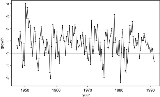
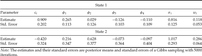
Employing the MSA model in equation (18) with p = 4 and using a Markov chain Monte Carlo method, McCulloch and Tsay (1994) obtain the estimates shown in Table 1. The results have several interesting findings. First, the mean growth rate of the marginal model for state 1 is 0.909/(1 − 0.265 − 0.029 + 0.126 + 0.11) = 0.965 and that of state 2 is −0.42/(1 − 0.216 − 0.628 + 0.073 + 0.097) = −1.288. Thus, state 1 corresponds to quarters with positive growth, or expansion periods, whereas state 2 consists of quarters with negative growth, or a contraction period. Second, the relatively large posterior standard deviations of the parameters in state 2 reflect that there are few observations in that state. This is expected as Figure 4 shows few quarters with negative growth. Third, the transition probabilities appear to be different for different states. The estimates indicate that it is more likely for the U.S. GNP to get out of a contraction period than to jump into one −0.286 versus 0.118. Fourth, treating 1/wi as the expected duration for the process to stay in state i, we see that the expected durations for a contraction period and an expansion period are approximately 3.69 and 11.31 quarters. Thus, on average, a contraction in the U.S. economy lasts about a year, whereas an expansion can last for 3 years. Finally, the estimated AR coefficients of xt−2 differ substantially between the two states, indicating that the dynamics of the U.S. economy are different between expansion and contraction periods.
Table 1 Estimation Results of a Markov Switching Model with p = 4 for the Growth Rate of U.S. Quarterly Real GNP, Seasonally Adjusted
Nonparametric Methods
In some financial applications, we may not have sufficient knowledge to prespecify the nonlinear structure between two variables Y and X. In other applications, we may wish to take advantage of the advances in computing facilities and computational methods to explore the functional relationship between Y and X. These considerations lead to the use of nonparametric methods and techniques. Nonparametric methods, however, are not without cost. They are highly data dependent and can easily result in overfitting. Our goal here is to introduce some nonparametric methods for financial applications and some nonlinear models that make use of nonparametric methods and techniques. The nonparametric methods discussed include kernel regression, local least squares estimation, and neural network.
The essence of nonparametric methods is smoothing. Consider two financial variables Y and X, which are related by
where m(.) is an arbitrary, smooth, but unknown function and {at} is a white noise sequence. We wish to estimate the nonlinear function m(.) from the data. For simplicity, consider the problem of estimating m(.) at a particular date for which X = x. That is, we are interested in estimating m(x). Suppose that at X = x we have repeated independent observations y1, … ,yT. Then the data become
![]()
Taking the average of the data, we have
![]()
By the law of large numbers, the average of the shocks converges to zero as T increases. Therefore, the average ![]() is a consistent estimate of m(x). That the average
is a consistent estimate of m(x). That the average ![]() provides a consistent estimate of m(x) or, alternatively, that the average of shocks converges to zero shows the power of smoothing.
provides a consistent estimate of m(x) or, alternatively, that the average of shocks converges to zero shows the power of smoothing.
In financial time series, we do not have repeated observations available at X = x. What we observed are {(yt, xt)} for t = 1, … , T. But if the function m(.) is sufficiently smooth, then the value of Yt for which Xt ![]() x continues to provide accurate approximation of m(x). The value of Yt for which Xt is far away from x provides less accurate approximation for m(x). As a compromise, one can use a weighted average of yt instead of the simple average to estimate m(x). The weight should be larger for those Yt with Xt close to x and smaller for those Yt with Xt far away from x. Mathematically, the estimate of m(x) for a given x can be written as
x continues to provide accurate approximation of m(x). The value of Yt for which Xt is far away from x provides less accurate approximation for m(x). As a compromise, one can use a weighted average of yt instead of the simple average to estimate m(x). The weight should be larger for those Yt with Xt close to x and smaller for those Yt with Xt far away from x. Mathematically, the estimate of m(x) for a given x can be written as
where the weights wt(x) are larger for those yt with xt close to x and smaller for those yt with xt far away from x. In equation (20), we assume that the weights sum to T. One can treat 1/T as part of the weights and make the weights sum to one.
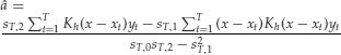
From equation (20), the estimate ![]() (x) is simply a local weighted average with weights determined by two factors. The first factor is the distance measure (i.e., the distance between xt and x). The second factor is the assignment of weight for a given distance. Different ways to determine the distance between xt and x and to assign the weight using the distance give rise to different nonparametric methods. In what follows, we discuss the commonly used kernel regression and local linear regression methods.
(x) is simply a local weighted average with weights determined by two factors. The first factor is the distance measure (i.e., the distance between xt and x). The second factor is the assignment of weight for a given distance. Different ways to determine the distance between xt and x and to assign the weight using the distance give rise to different nonparametric methods. In what follows, we discuss the commonly used kernel regression and local linear regression methods.
Kernel Regression
Kernel regression is perhaps the most commonly used nonparametric method in smoothing. The weights here are determined by a kernel, which is typically a probability density function, is denoted by K(x), and satisfies
![]()
However, to increase the flexibility in distance measure, one often rescales the kernel using a variable h > 0, which is referred to as the bandwidth. The rescaled kernel becomes
The weight function can now be defined as
where the denominator is a normalization constant that makes the smoother adaptive to the local intensity of the X variable and ensures the weights sum to one. Plugging equation (22) into the smoothing formula (20), we have the well-known Nadaraya-Watson kernel estimator
(23) ![]()
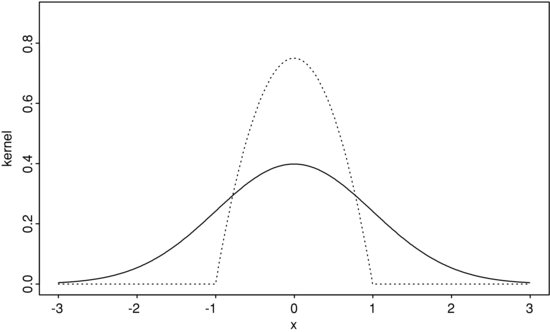
see Nadaraya (1964) and Watson (1964). In practice, many choices are available for the kernel K(x). However, theoretical and practical considerations lead to a few choices, including the Gaussian kernel
![]()
and the Epanechnikov kernel (Epanechnikov, 1969)
![]()
where 1(A) is an indicator such that 1(A) = 1 if A holds and 1(A) = 0 otherwise. Figure 5 shows the Gaussian and Epanechnikov kernels for h = 1.
Figure 5 Standard Normal Kernel (Solid Line) and Epanechnikov Kernel (Dashed Line) with Bandwidth h = 1
To gain insight into the bandwidth h, we evaluate the Nadaraya-Watson estimator with the Epanechnikov kernel at the observed values {xt} and consider two extremes. First, if h → 0, then
![]()
indicating that small bandwidths reproduce the data. Second, if h →∞, then
![]()
suggesting that large bandwidths lead to an oversmoothed curve—the sample mean. In general, the bandwidth function h acts as follows. If h is very small, then the weights focus on a few observations that are in the neighborhood around each xt. If h is very large, then the weights will spread over a larger neighborhood of xt. Consequently, the choice of h plays an important role in kernel regression. This is the well-known problem of bandwidth selection in kernel regression.
Bandwidth Selection
There are several approaches for bandwidth selection; see Härdle (1990) and Fan and Yao (2003). The first approach is the plug-in method, which is based on the asymptotic expansion of the mean integrated squared error (MISE) for kernel smoothers
![]()
where m(.) is the true function. The quantity ![]() of the MISE is a pointwise measure of the mean squared error (MSE) of
of the MISE is a pointwise measure of the mean squared error (MSE) of ![]() (x) evaluated at x.
(x) evaluated at x.
Under some regularity conditions, one can derive the optimal bandwidth that minimizes the MISE. The optimal bandwidth typically depends on several unknown quantities that must be estimated from the data with some preliminary smoothing. Several iterations are often needed to obtain a reasonable estimate of the optimal bandwidth. In practice, the choice of preliminary smoothing can become a problem. Fan and Yao (2003) give a normal reference bandwidth selector as
![]()
where s is the sample standard error of the indepenent variable, which is assumed to be stationary.
The second approach to bandwidth selection is the leave-one-out cross-validation. First, one observation (xj, yj) is left out. The remaining T − 1 data points are used to obtain the following smoother at xj:
![]()
which is an estimate of yj, where the weights wt(xj) sum to T−1. Second, perform step-1 for j = 1, … , T and define the function
![]()
where w(.) is a nonnegative weight function satisfying ![]() , that can be used to down-weight the boundary points if necessary. Decreasing the weights assigned to data points close to the boundary is needed because those points often have fewer neighboring observations. The function CV(h) is called the cross-validation function because it validates the ability of the smoother to predict {yt}Tt=1. One chooses the bandwidth h that minimizes the CV(.) function.
, that can be used to down-weight the boundary points if necessary. Decreasing the weights assigned to data points close to the boundary is needed because those points often have fewer neighboring observations. The function CV(h) is called the cross-validation function because it validates the ability of the smoother to predict {yt}Tt=1. One chooses the bandwidth h that minimizes the CV(.) function.
Local Linear Regression Method
Assume that the second derivative of m(.) in model (19) exists and is continuous at x, where x is a given point in the support of m(.). Denote the data available by ![]() . The local linear regression method to nonparametric regression is to find a and b that minimize
. The local linear regression method to nonparametric regression is to find a and b that minimize
where Kh(.) is a kernel function defined in equation (21) and h is a bandwidth. Denote the resulting value of a by ![]() . The estimate of m(x) is then defined as
. The estimate of m(x) is then defined as ![]() . In practice, x assumes an observed value of the independent variable. The estimate
. In practice, x assumes an observed value of the independent variable. The estimate ![]() can be used as an estimate of the first derivative of m(.) evaluated at x.
can be used as an estimate of the first derivative of m(.) evaluated at x.
Under the least squares theory, equation (24) is a weighted least squares problem and one can derive a closed-form solution for a. Specifically, taking the partial derivatives of L(a, b) with respect to both a and b and equating the derivatives to zero, we have a system of two equations with two unknowns:
Define
![]()
The prior system of equations becomes
Consequently, we have
The numerator and denominator of the prior fraction can be further simplified as

In summary, we have
(25) ![]()
where wt is defined as
![]()
In practice, to avoid possible zero in the denominator, we use ![]() (x) next to estimate m(x):
(x) next to estimate m(x):
Notice that a nice feature of equation (26) is that the weight wt satisfies
![]()
Also, if one assumes that m(.) of equation (19) has the first derivative and finds the minimizer of
![]()
then the resulting estimator is the Nadaraya-Watson estimator mentioned earlier. In general, if one assumes that m(x) has a bounded kth derivative, then one can replace the linear polynomial in equation (24) by a (k − 1)-order polynomial. We refer to the estimator in equation (26) as the local linear regression smoother. Fan (1993) shows that, under some regularity conditions, the local linear regression estimator has some important sampling properties. The selection of bandwidth can be carried out via the same methods as before.
Financial Time Series Application
In time series analysis, the explanatory variables are often the lagged values of the series. Consider the simple case of a single explanatory variable. Here model (19) becomes
![]()
and the kernel regression and local linear regression method discussed before are directly applicable. When multiple explanatory variables exist, some modifications are needed to implement the nonparametric methods. For the kernel regression, one can use a multivariate kernel such as a multivariate normal density function with a prespecified covariance matrix:
![]()
where p is the number of explanatory variables and Σ is a prespecified positive-definite matrix. Alternatively, one can use the product of univariate kernel functions as a multivariate kernel—for example,
![]()
This latter approach is simple, but it overlooks the relationship between the explanatory variables.
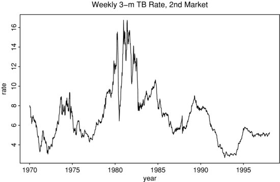
Example 6. To illustrate the application of nonparametric methods in finance, consider the weekly 3-month Treasury bill secondary market rate from 1970 to 1997 for 1,461 observations. The data are obtained from the Federal Reserve Bank of St. Louis and are shown in Figure 6. This series has been used in the literature as an example of estimating stochastic diffusion equations using discretely observed data. Here we consider a simple model
![]()
where xt is the 3-month Treasury bill rate, yt = xt − xt−1, wt is a standard Brownian motion, and μ(.) and σ(.) are smooth functions of xt−1, and apply the local smoothing function lowess of R or S-Plus to obtain nonparametric estimates of μ(.) and σ(.); see Cleveland (1979). For simplicity, we use |yt| as a proxy of the volatility of xt.
Figure 6 Time Plot of U.S. Weekly 3-Month Treasury Bill Rate in the Seconday Market from 1970 to 1997
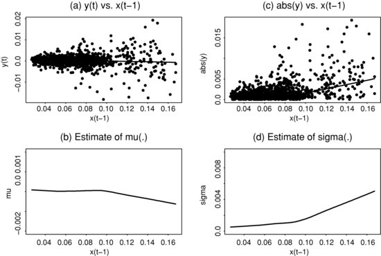
For the simple model considered, μ(xt−1) is the conditional mean of yt given xt−1, that is, μ(xt−1) = E(yt|xt−1). Figure 7(a) shows the scatterplot of y(t) versus xt−1. The plot also contains the local smooth estimate of μ(xt−1) obtained by the method of lowess in the statistical package R. The estimate is essentially zero. However, to better understand the estimate, Figure 7(b) shows the estimate ![]() on a finer scale. It is interesting to see that
on a finer scale. It is interesting to see that ![]() is positive when xt−1 is small, but becomes negative when xt−1 is large. This is in agreement with the common sense that when the interest rate is high, it is expected to come down, and when the rate is low, it is expected to increase. Figure 7(c) shows the scatterplot of |y(t)| versus xt−1 and the estimate of
is positive when xt−1 is small, but becomes negative when xt−1 is large. This is in agreement with the common sense that when the interest rate is high, it is expected to come down, and when the rate is low, it is expected to increase. Figure 7(c) shows the scatterplot of |y(t)| versus xt−1 and the estimate of ![]() (xt−1) via lowess. The plot confirms that the higher the interest rate, the larger the volatility. Figure 7(d) shows the estimate
(xt−1) via lowess. The plot confirms that the higher the interest rate, the larger the volatility. Figure 7(d) shows the estimate ![]() (xt−1) on a finer scale. Clearly the volatility is an increasing function of xt−1 and the slope seems to accelerate when xt−1 is approaching 10%. This example demonstrates that simple non-parametric methods can be helpful in understanding the dynamic structure of a financial time series.
(xt−1) on a finer scale. Clearly the volatility is an increasing function of xt−1 and the slope seems to accelerate when xt−1 is approaching 10%. This example demonstrates that simple non-parametric methods can be helpful in understanding the dynamic structure of a financial time series.
Figure 7 Estimation of Conditional Mean and Volatility of Weekly 3-Month Treasury Bill Rate via a Local Smoothing Method: (a) yt versus xt−1, where yt = xt−xt−1 and xt is the interest rate; (b) estimate of μ(xt−1); (c) |yt| versus xt−1; and (d) estimate of σ(xt−1)
The following nonlinear models are derived with the help of nonparametric methods.
Functional Coefficient AR Model
Recent advances in nonparametric techniques enable researchers to relax parametric constraints in proposing nonlinear models. In some cases, nonparametric methods are used in a preliminary study to help select a parametric nonlinear model. This is the approach taken by Chen and Tsay (1993a) in proposing the functional-coefficient autoregressive (FAR) model that can be written as
where Xt−1 = (xt−1, … , Xt−k)′ is a vector of lagged values of xt. If necessary xt−1 may also include other explanatory variables available at time t−1. The functions fi(.) of equation (27) are assumed to be continuous, even twice differentiable, almost surely with respect to their arguments. Most of the nonlinear models discussed before are special cases of the FAR model. In application, one can use nonparametric methods such as kernel regression or local linear regression to estimate the functional coefficients fi(.), especially when the dimension of Xt−1 is low (e.g., Xt−1 is a scalar). Recently, Cai, Fan, and Yao (2000) applied the local linear regression method to estimate fi(.) and showed that substantial improvements in 1-step ahead forecasts can be achieved by using FAR models.
Nonlinear Additive AR Model
A major difficulty in applying nonparametric methods to nonlinear time series analysis is the “curse of dimensionality.” Consider a general nonlinear AR(p) process xt = f(xt−1, … , xt−p) + at. A direct application of nonparametric methods to estimate f(.) would require p-dimensional smoothing, which is hard to do when p is large, especially if the number of data points is not large. A simple, yet effective way to overcome this difficulty is to entertain an additive model that only requires lower dimensional smoothing. A time series xt follows a nonlinear additive AR (NAAR) model if
(28) ![]()
where the fi(.) are continuous functions almost surely. Because each function fi(.) has a single argument, it can be estimated nonparametrically using one-dimensional smoothing techniques and hence avoids the curse of dimensionality. In application, an iterative estimation method that estimates fi(.) nonparametrically conditioned on estimates of fj(.) for all j ≠ i is used to estimate a NAAR model; see Chen and Tsay (1993b) for further details and examples of NAAR models.
The additivity assumption is rather restrictive and needs to be examined carefully in application. Chen, Liu, and Tsay (1995) consider test statistics for checking the additivity assumption.
Nonlinear State-Space Model
Making using of recent advances in MCMC methods (Gelfand and Smith, 1990), Carlin, Polson, and Stoffer (1992) propose a Monte Carlo approach for nonlinear state-space modeling. The model considered is
where St is the state vector, ft(.) and gt(.) are known functions depending on some unknown parameters, {ut} is a sequence of IID multivariate random vectors with zero mean and nonnegative definite covariance matrix Σu, {vt} is a sequence of IID random variables with mean zero and variance ![]() , and {ut} is independent of {vt}.
, and {ut} is independent of {vt}.
Monte Carlo techniques are employed to handle the nonlinear evolution of the state transition equation because the whole conditional distribution function of St given St−1 is needed for a nonlinear system. Other numerical smoothing methods for nonlinear time series analysis have been considered by Kitagawa (1998) and the references therein. MCMC methods (or computing-intensive numerical methods) are powerful tools for nonlinear time series analysis. Their potential has not been fully explored. However, the assumption of knowing ft(.) and gt(.) in model (29) may hinder practical use of the proposed method. A possible solution to overcome this limitation is to use nonparametric methods such as the analyses considered in FAR and NAAR models to specify ft(.) and gt(.) before using nonlinear state-space models.
Neural Networks
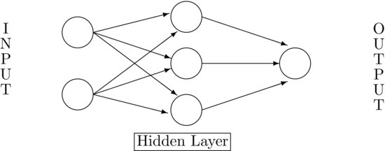
A popular topic in modern data analysis is neural network, which can be classified as a semiparametric method. The literature on neural network is enormous, and its application spreads over many scientific areas with varying degrees of success; see Ripley (1993, Sections 2 and 10). Cheng and Titterington (1994) provide information on neural networks from a statistical viewpoint. In this subsection, we focus solely on the feed-forward neural networks in which inputs are connected to one or more neurons, or nodes, in the input layer, and these nodes are connected forward to further layers until they reach the output layer. Figure 8 shows an example of a simple feed-forward network for univariate time series analysis with one hidden layer. The input layer has two nodes, and the hidden layer has three. The input nodes are connected forward to each and every node in the hidden layer, and these hidden nodes are connected to the single node in the output layer. We call the network a 2-3-1 feed-forward network. More complicated neural networks, including those with feedback connections, have been proposed in the literature, but the feed-forward networks are most relevant to our study.
Figure 8 A Feed-Forward Neural Network with One Hidden Layer for Univariate Time Series Analysis
Feed-Forward Neural Networks
A neural network processes information from one layer to the next by an “activation function.” Consider a feed-forward network with one hidden layer. The jth node in the hidden layer is defined as
(30) ![]()
where xi is the value of the ith input node, fj(.) is an activation function typically taken to be the logistic function
![]()
α0j is called the bias, the summation i → j means summing over all input nodes feeding to j, and wij are the weights. For illustration, the jth node of the hidden layer of the 2-3-1 feed-forward network in Figure 8 is
For the output layer, the node is defined as
(32) ![]()
where the activation function fo(.) is either linear or a Heaviside function. If fo(.) is linear, then
![]()
where k is the number of nodes in the hidden layer. By a Heaviside function, we mean fo(z) = 1 if z > 0 and fo(z) = 0 otherwise. A neuron with a Heaviside function is called a threshold neuron, with “1” denoting that the neuron fires its message. For example, the output of the 2-3-1 network in Figure 8 is
![]()
if the activation function is linear; it is
![]()
if fo(.) is a Heaviside function.
Combining the layers, the output of a feed-forward neural network can be written as
If one also allows for direct connections from the input layer to the output layer, then the network becomes
where the first summation is summing over the input nodes. When the activation function of the output layer is linear, the direct connections from the input nodes to the output node represent a linear function between the inputs and output. Consequently, in this particular case model (34) is a generalization of linear models. For the 2-3-1 network in Figure 8, if the output activation function is linear, then equation (33) becomes
![]()
where hj is given in equation (31). The network thus has 13 parameters. If equation (34) is used, then the network becomes
![]()
where again hj is given in equation (31). The number of parameters of the network increases to 15.
We refer to the function in equation (33) or (34) as a semiparametric function because its functional form is known, but the number of nodes and their biases and weights are unknown. The direct connections from the input layer to the output layer in equation (34) mean that the network can skip the hidden layer. We refer to such a network as a skip-layer feed-forward network.
Feed-forward networks are known as multilayer percetrons in the neural network literature. They can approximate any continuous function uniformly on compact sets by increasing the number of nodes in the hidden layer; see Hornik, Stinchcombe, and White (1989), Hornik (1993), and Chen and Chen (1995). This property of neural networks is the universal approximation property of the multilayer percetrons. In short, feed-forward neural networks with a hidden layer can be seen as a way to parameterize a general continuous nonlinear function.
Training and Forecasting
Application of neural networks involves two steps. The first step is to train the network (i.e., to build a network, including determining the number of nodes and estimating their biases and weights). The second step is inference, especially forecasting. The data are often divided into two nonoverlapping subsamples in the training stage. The first subsample is used to estimate the parameters of a given feed-forward neural network. The network so built is then used in the second subsample to perform forecasting and compute its forecasting accuracy. By comparing the forecasting performance, one selects the network that outperforms the others as the “best” network for making inference. This is the idea of cross-validation widely used in statistical model selection. Other model selection methods are also available.
In a time series application, let {(rt, xt)|t = 1, … , T} be the available data for network training, where xt denotes the vector of inputs and rt is the series of interest (e.g., log returns of an asset). For a given network, let ot be the output of the network with input xt; see equation (34). Training a neural network amounts to choosing its biases and weights to minimize some fitting criterion—for example, the least squares
![]()
This is a nonlinear estimation problem that can be solved by several iterative methods. To ensure the smoothness of the fitted function, some additional constraints can be added to the prior minimization problem. In the neural network literature, the back propagation (BP) learning algorithm is a popular method for network training. The BP method, introduced by Bryson and Ho (1969), works backward starting with the output layer and uses a gradient rule to modify the biases and weights iteratively. (Appendix 2A of Ripley, 1993, provides a derivation of back propagation.) Once a feed-forward neural network is built, it can be used to compute forecasts in the forecasting subsample.
Example 7. To illustrate applications of the neural network in finance, we consider the monthly log returns, in percentages and including dividends, for IBM stock from January 1926 to December 1999. We divide the data into two subsamples. The first subsample consisting of returns from January 1926 to December 1997 for 864 observations is used for modeling. Using model (34) with three inputs and two nodes in the hidden layer, we obtain a 3-2-1 network for the series. The three inputs are rt−1, rt−2, and rt−3 and the biases and weights are given next:
where rt−1 = (rt−1, rt−2, rt−3) and the two logistic functions are
The standard error of the residuals for the prior model is 6.56. For comparison, we also built an AR model for the data and obtained
The residual standard error is slightly greater than that of the feed-forward model in equation (35).
Forecast Comparison
The monthly returns of IBM stock in 1998 and 1999 form the second subsample and are used to evaluate the out-of-sample forecasting performance of neural networks. As a benchmark for comparison, we use the sample mean of rt in the first subsample as the 1-step ahead forecast for all the monthly returns in the second subsample. This corresponds to assuming that the log monthly price of IBM stock follows a random walk with drift. The mean squared forecast error (MSFE) of this benchmark model is 91.85. For the AR(1) model in equation (36), the MSFE of 1-step ahead forecasts is 91.70. Thus, the AR(1) model slightly outperforms the benchmark. For the 3-2-1 feed-forward network in equation (35), the MSFE is 91.74, which is essentially the same as that of the AR(1) model.
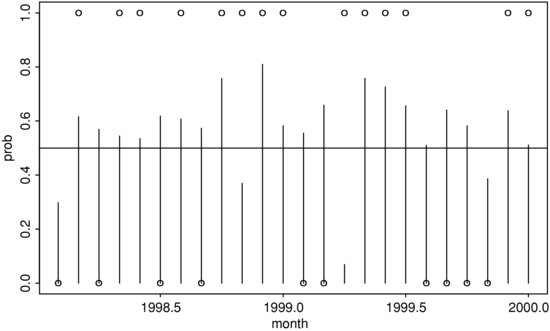
Example 8. Nice features of the feed-forward network include its flexibility and wide applicability. For illustration, we use the network with a Heaviside activation function for the output layer to forecast the direction of price movement for IBM stock considered in Example 7. Define a direction variable as
![]()
We use eight input nodes consisting of the first four lagged values of both rt and dt and four nodes in the hidden layer to build an 8-4-1 feed-forward network for dt in the first subsample. The resulting network is then used to compute the 1-step ahead probability of an “upward movement” (i.e., a positive return) for the following month in the second subsample.
Figure 9 shows a typical output of probability forecasts and the actual directions in the second subsample with the latter denoted by circles. A horizontal line of 0.5 is added to the plot. If we take a rigid approach by letting ![]() = 1 if the probability forecast is greater than or equal to 0.5 and
= 1 if the probability forecast is greater than or equal to 0.5 and ![]() = 0 otherwise, then the neural network has a successful rate of 0.58. The success rate of the network varies substantially from one estimation to another, and the network uses 49 parameters.
= 0 otherwise, then the neural network has a successful rate of 0.58. The success rate of the network varies substantially from one estimation to another, and the network uses 49 parameters.
Figure 9 One-Step Ahead Probability Forecasts for a Positive Monthly Return for IBM Stock Using an 8-4-1 Feed-Forward Neural Network
Note: The forecasting period is from January 1998 to December 1999.
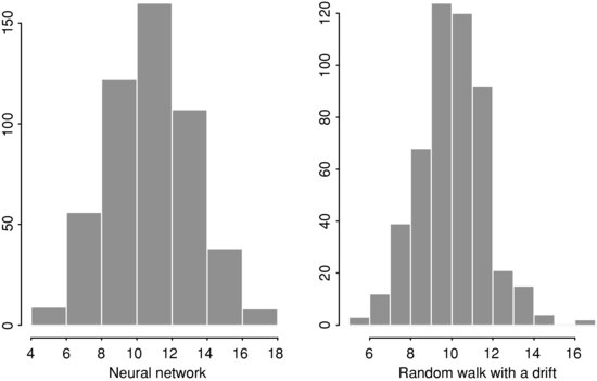
To gain more insight, we did a simulation study of running the 8-4-1 feed-forward network 500 times and computed the number of errors in predicting the upward and downward movement using the same method as before. The mean and median of errors over the 500 runs are 11.28 and 11, respectively, whereas the maximum and minimum number of errors are 18 and 4. For comparison, we also did a simulation with 500 runs using a random walk with drift—that is,
![]()
where 1.19 is the average monthly log return for IBM stock from January 1926 to December 1997 and {![]() t} is a sequence of IID N(0,1) random variables. The mean and median of the number of forecast errors become 10.53 and 11, whereas the maximum and minimum number of errors are 17 and 5, respectively. Figure 10 shows the histograms of the number of forecast errors for the two simulations. The results show that the 8-4-1 feed-forward neural network does not outperform the simple model that assumes a random walk with drift for the monthly log price of IBM stock.
t} is a sequence of IID N(0,1) random variables. The mean and median of the number of forecast errors become 10.53 and 11, whereas the maximum and minimum number of errors are 17 and 5, respectively. Figure 10 shows the histograms of the number of forecast errors for the two simulations. The results show that the 8-4-1 feed-forward neural network does not outperform the simple model that assumes a random walk with drift for the monthly log price of IBM stock.
Figure 10 Histograms of the Number of Forecasting Errors for the Directional Movements of Monthly Log Returns of IBM Stock
Note: The forecasting period is from January 1998 to December 1999.
NONLINEARITY TESTS
In this section, we discuss some nonlinearity tests available in the literature that have decent power against the nonlinear models considered earlier in this entry. The tests discussed include both parametric and nonparametric statistics. The Ljung-Box statistics of squared residuals, the bispectral test, and the Brock, Dechert, and Scheinkman (BDS) test are nonparametric methods. The RESET test (Ramsey, 1969), the F tests of Tsay (1986, 1989), and other Lagrange multiplier and likelihood ratio tests depend on specific parametric functions. Because nonlinearity may occur in many ways, there exists no single test that dominates the others in detecting nonlinearity.
Nonparametric Tests
Under the null hypothesis of linearity, residuals of a properly specified linear model should be independent. Any violation of independence in the residuals indicates inadequacy of the entertained model, including the linearity assumption. This is the basic idea behind various nonlinearity tests. In particular, some of the nonlinearity tests are designed to check for possible violation in quadratic forms of the underlying time series.
Q-Statistic of Squared Residuals
McLeod and Li (1983) apply the Ljung-Box statistics to the squared residuals of an ARMA(p, q) model to check for model inadequacy. The test statistic is
![]()
where T is the sample size, m is a properly chosen number of autocorrelations used in the test, at denotes the residual series, and ![]() is the lag-i ACF of a2t. If the entertained linear model is adequate, Q(m) is asymptotically a chi-squared random variable with m—p—q degrees of freedom. The prior Q-statistic is useful in detecting conditional heteroscedasticity of at and is asymptotically equivalent to the Lagrange multiplier test statistic of Engle (1982) for ARCH models. The null hypothesis of the statistics is Ho : β1 = … = βm = 0, where βi is the coefficient of a2t-i in the linear regression
is the lag-i ACF of a2t. If the entertained linear model is adequate, Q(m) is asymptotically a chi-squared random variable with m—p—q degrees of freedom. The prior Q-statistic is useful in detecting conditional heteroscedasticity of at and is asymptotically equivalent to the Lagrange multiplier test statistic of Engle (1982) for ARCH models. The null hypothesis of the statistics is Ho : β1 = … = βm = 0, where βi is the coefficient of a2t-i in the linear regression
![]()
for t = m + 1, … ,T. Because the statistic is computed from residuals (not directly from the observed returns), the number of degrees of freedom is m—p—q.
Bispectral Test
This test can be used to test for linearity and Gaussianity. It depends on the result that a properly normalized bispectrum of a linear time series is constant over all frequencies and that the constant is zero under normality. The bispectrum of a time series is the Fourier transform of its third-order moments. For a stationary time series xt in equation (1), the third-order moment is defined as
where u and v are integers, ![]() , ψ0 = 1, and ψk = 0 for k < 0. Taking Fourier transforms of equation (37), we have
, ψ0 = 1, and ψk = 0 for k < 0. Taking Fourier transforms of equation (37), we have
(38) ![]()
where ![]() exp(−iwu) with i =
exp(−iwu) with i = ![]() , and wi are frequencies. Yet the spectral density function of xt is given by
, and wi are frequencies. Yet the spectral density function of xt is given by
![]()
where w denotes the frequency. Consequently, the function

The bispectrum test makes use of the property in equation (39). Basically, it estimates the function b(w1, w2) in equation (39) over a suitably chosen grid of points and applies a test statistic similar to Hotelling’s T2 statistic to check the constancy of b(w1, w2). For a linear Gaussian series, ![]() so that the bispectrum is zero for all frequencies (w1, w2). For further details of the bispectral test, see Priestley (1988), Subba Rao and Gabr (1984), and Hinich (1982). Limited experience shows that the test has decent power when the sample size is large.
so that the bispectrum is zero for all frequencies (w1, w2). For further details of the bispectral test, see Priestley (1988), Subba Rao and Gabr (1984), and Hinich (1982). Limited experience shows that the test has decent power when the sample size is large.
BDS Statistic
Brock, Dechert, and Scheinkman (1987) propose a test statistic, commonly referred to as the BDS test, to detect the IID assumption of a time series. The statistic is, therefore, different from other test statistics discussed because the latter mainly focus on either the second- or third-order properties of xt. The basic idea of the BDS test is to make use of a “correlation integral” popular in chaotic time series analysis. Given a k-dimensional time series Xt and observations ![]() , define the correlation integral as
, define the correlation integral as
(40) ![]()
where Iδ(u, v) is an indicator variable that equals one if ||u—v|| < δ, and zero otherwise, where ||.|| is the supnorm. The correlation integral measures the fraction of data pairs of {Xt} that are within a distance of δ from each other.
Consider next a time series xt. Construct k-dimensional vectors ![]() which are called k-histories. The idea of the BDS test is as follows. Treat a k-history as a point in the k-dimensional space. If
which are called k-histories. The idea of the BDS test is as follows. Treat a k-history as a point in the k-dimensional space. If ![]() are indeed IID random variables, then the k-histories
are indeed IID random variables, then the k-histories ![]() should show no pattern in the k-dimensional space. Consequently, the correlation integrals should satisfy the relation
should show no pattern in the k-dimensional space. Consequently, the correlation integrals should satisfy the relation ![]() . Any departure from the prior relation suggests that xt are not IID. As a simple but informative example, consider a sequence of IID random variables from the uniform distribution over [0, 1]. Let [a, b] be a subinterval of [0, 1] and consider the “2-history” (xt, xt+1), which represents a point in the two-dimensional space. Under the IID assumption, the expected number of 2-histories in the subspace [a, b] × [a, b] should equal the square of the expected number of xt in [a, b].
. Any departure from the prior relation suggests that xt are not IID. As a simple but informative example, consider a sequence of IID random variables from the uniform distribution over [0, 1]. Let [a, b] be a subinterval of [0, 1] and consider the “2-history” (xt, xt+1), which represents a point in the two-dimensional space. Under the IID assumption, the expected number of 2-histories in the subspace [a, b] × [a, b] should equal the square of the expected number of xt in [a, b].
This idea can be formally examined by using sample counterparts of correlation integrals. Define
![]()
where ![]() and X*i = xi if l = 1 and X*i = Xki if l = k. Under the null hypothesis that {xt} are IID with a nondegenerated distribution function F(.), Brock, Dechert, and Scheinkman (1987) show that
and X*i = xi if l = 1 and X*i = Xki if l = k. Under the null hypothesis that {xt} are IID with a nondegenerated distribution function F(.), Brock, Dechert, and Scheinkman (1987) show that
![]()
for any fixed k and δ. Furthermore, the statistic ![]() is asymptotically distributed as normal with mean zero and variance
is asymptotically distributed as normal with mean zero and variance
where ![]() and
and ![]() . Note that C1{δ, T) is a consistent estimate of C, and N can be consistently estimated by
. Note that C1{δ, T) is a consistent estimate of C, and N can be consistently estimated by
The BDS test statistic is then defined as
(41) ![]()
where σk(δ, T) is obtained from σk(δ) when C and N are replaced by C1(δ, T) and N(δ, T), respectively. This test statistic has a standard normal limiting distribution. For further discussion and examples of applying the BDS test, see Hsieh (1989) and Brock, Hsieh, and LeBaron (1991). In application, one should remove linear dependence, if any, from the data before applying the BDS test. The test may be sensitive to the choices of δ and k, especially when k is large.
Parametric Tests
Turning to parametric tests, we consider the RESET test of Ramsey (1969) and its generalizations. We also discuss some test statistics for detecting threshold nonlinearity.
The RESET Test
Ramsey (1969) proposes a specification test for linear least squares regression analysis. The test is referred to as a RESET test and is readily applicable to linear AR models. Consider the linear AR(p) model
where Xt−1 = (1, xt−1, … , xt−p)′ and ![]() = (
= (![]() 0,
0, ![]() 1, … ,
1, … , ![]() p)’. The first step of the RESET test is to obtain the least squares estimate
p)’. The first step of the RESET test is to obtain the least squares estimate ![]() of equation (42) and compute the fit
of equation (42) and compute the fit ![]() , the residual
, the residual ![]() , and the sum of squared residuals
, and the sum of squared residuals ![]() , where T is the sample size. In the second step, consider the linear regression
, where T is the sample size. In the second step, consider the linear regression
where ![]() for some s ≥ 1, and compute the least squares residuals
for some s ≥ 1, and compute the least squares residuals
![]()
and the sum of squared residuals SSR1![]() of the regression. The basic idea of the RESET test is that if the linear AR(p) model in equation (42) is adequate, then α1 and α2 of equation (43) should be zero. This can be tested by the usual F statistic of equation (43) given by
of the regression. The basic idea of the RESET test is that if the linear AR(p) model in equation (42) is adequate, then α1 and α2 of equation (43) should be zero. This can be tested by the usual F statistic of equation (43) given by
(44) ![]()
which, under the linearity and normality assumption, has an F distribution with degrees of freedom g and T − p − g.
Because ![]() for k = 2, … , s + 1 tend to be highly correlated with Xt−1 and among themselves, principal components of Mt−1 that are not colinear with Xt−1 are often used in fitting equation (43).
for k = 2, … , s + 1 tend to be highly correlated with Xt−1 and among themselves, principal components of Mt−1 that are not colinear with Xt−1 are often used in fitting equation (43).
Keenan (1985) proposes a nonlinearity test for time series that uses ![]() only and modifies the second step of the RESET test to avoid multicollinearity between
only and modifies the second step of the RESET test to avoid multicollinearity between ![]() and Xt−1. Specifically the linear regression (43) is divided into two steps. In step 2(a), one removes linear dependence of
and Xt−1. Specifically the linear regression (43) is divided into two steps. In step 2(a), one removes linear dependence of ![]() on Xt−1 by fitting the regression
on Xt−1 by fitting the regression
![]()
and obtaining the residual ![]() . In step 2(b), consider the linear regression
. In step 2(b), consider the linear regression
![]()
and obtain the sum of squared residuals SSR1 = ![]() to test the null hypothesis α = 0.
to test the null hypothesis α = 0.
The F Test
To improve the power of Keenan’s test and the RESET test, Tsay (1986) uses a different choice of the regressor Mt−1. Specifically, he suggests using Mt−1 = vech![]() , where vech(A) denotes the half-stacking vector of the matrix A using elements on and below the diagonal only. For example, if p = 2, then Mt−1 =
, where vech(A) denotes the half-stacking vector of the matrix A using elements on and below the diagonal only. For example, if p = 2, then Mt−1 = ![]() . The dimension of Mt−1 is p(p + 1)/2 for an AR(p) model. In practice, the test is simply the usual partial F statistic for testing α = 0 in the linear least squares regression
. The dimension of Mt−1 is p(p + 1)/2 for an AR(p) model. In practice, the test is simply the usual partial F statistic for testing α = 0 in the linear least squares regression
![]()
where et denotes the error term. Under the assumption that xt is a linear AR(p) process, the partial F statistic follows an F distribution with degrees of freedom g and T − p − g − 1, where g = p(p + 1)/2. We refer to this F test as the Ori-F test. Luukkonen, Saikkonen, and Teräsvirta (1988) further extend the test by augmenting Mt−1 with cubic terms ![]() for i = 1, … , p.
for i = 1, … , p.
Threshold Test
When the alternative model under study is a SETAR model, one can derive specific test statistics to increase the power of the test. One of the specific tests is the likelihood ratio statistic. This test, however, encounters the difficulty of undefined parameters under the null hypothesis of linearity because the threshold is undefined for a linear AR process. Another specific test seeks to transform testing threshold nonlinearity into detecting model changes. It is then interesting to discuss the differences between these two specific tests for threshold nonlinearity.
To simplify the discussion, let us consider the simple case that the alternative model is a 2-regime SETAR model with threshold variable xt−d. The null hypothesis Ho: xt follows the linear AR(p) model
(45) ![]()
whereas the alternative hypothesis Ha : xt follows the SETAR model
where r1 is the threshold. For a given realization ![]() and assuming normality let
and assuming normality let ![]() be the log likelihood function evaluated at the maximum likelihood estimates of
be the log likelihood function evaluated at the maximum likelihood estimates of ![]() = (
= (![]() 0, … ,
0, … ,![]() p)′ and
p)′ and ![]() This is easy to compute. The likelihood function under the alternative is also easy to compute if the threshold r1 is given. Let
This is easy to compute. The likelihood function under the alternative is also easy to compute if the threshold r1 is given. Let ![]() be the log likelihood function evaluated at the maximum likelihood estimates of
be the log likelihood function evaluated at the maximum likelihood estimates of ![]() and
and ![]() conditioned on knowing the threshold r1. The log likelihood ratio l(r1) defined as
conditioned on knowing the threshold r1. The log likelihood ratio l(r1) defined as
![]()
is then a function of the threshold r1, which is unknown. Yet under the null hypothesis, there is no threshold and r1 is not defined. The parameter r1 is referred to as a nuisance parameter under the null hypothesis. Consequently, the asymptotic distribution of the likelihood ratio is very different from that of the conventional likelihood ratio statistics. (See Chan, 1991, for further details and critical values of the test.) A common approach is to use lmax = supv < r1 < u l(r1) as the test statistic, where v and u are prespecifled lower and upper bounds of the threshold. Davis (1987) and Andrews and Ploberger (1994) provide further discussion on hypothesis testing involving nuisance parameters under the null hypothesis. Simulation is often used to obtain empirical critical values of the test statistic lmax, which depends on the choices of v and u. The average of l(r1) over r1 ![]() [v, u] is also considered by Andrews and Ploberger as a test statistic.
[v, u] is also considered by Andrews and Ploberger as a test statistic.
Tsay (1989) makes use of arranged autoregression and recursive estimation tio derive an alternative test for threshold nonlinearity. The arranged autoregression seeks to transfer the SETAR model under the alternative hypothesis Ha into a model change problem with the threshold r1 serving as the change point. To see this, the SETAR model in equation (46) says that xt follows essentially two linear models depending on whether xt−d < r1 or xt−d ≥ r1. For a realization ![]() can assume values {x1, … , XT−d}. Let x(1) ≤ x(2) ≤ … ≤ x(T−d) be the ordered statistics of
can assume values {x1, … , XT−d}. Let x(1) ≤ x(2) ≤ … ≤ x(T−d) be the ordered statistics of ![]() (i.e., arranging the observations in increasing order). The SETAR model can then be written as
(i.e., arranging the observations in increasing order). The SETAR model can then be written as

where ![]() if x(j) < r1 and
if x(j) < r1 and ![]() if
if ![]() r1. Consequently, the threshold r1 is a change point for the linear regression in equation (47), and we refer to equation (47) as an arranged autoregression (in increasing order of the threshold xt−d). Note that the arranged autoregression in (47) does not alter the dynamic dependence of xt on xt−i for i = 1, … , p because x(j)+d still depends on x(j)+d−i for i = 1, … , p. What is done is simply to present the SETAR model in the threshold space instead of in the time space. That is, the equation with a smaller xt−d appears before that with a larger xt−d. The threshold test of Tsay (1989) is obtained as follows.
r1. Consequently, the threshold r1 is a change point for the linear regression in equation (47), and we refer to equation (47) as an arranged autoregression (in increasing order of the threshold xt−d). Note that the arranged autoregression in (47) does not alter the dynamic dependence of xt on xt−i for i = 1, … , p because x(j)+d still depends on x(j)+d−i for i = 1, … , p. What is done is simply to present the SETAR model in the threshold space instead of in the time space. That is, the equation with a smaller xt−d appears before that with a larger xt−d. The threshold test of Tsay (1989) is obtained as follows.
- Step 1. Fit equation (47) using j = 1, … , m, where m is a prespecified positive integer (e.g., 30). Denote the least squares estimates of βi by
 where m denotes the number of data points used in estimation.
 - Step 2. Compute the predictive residual
and its standard error. Let
 be the standardized predictive residual.
 - Step 3. Use the recursive least squares method to update the least squares estimates to
 by incorporating the new data point x(m+1)+d.
 - Step 4. Repeat steps 2 and 3 until all data points are processed.
- Step 5. Consider the linear regression of the standardized predictive residual
and compute the usual F statistic for testing αi = 0 in equation (48) for i = 0, … ,p. Under the null hypothesis that xt follows a linear AR(p) model, the F ratio has a limiting F distribution with degrees of freedom p + 1 and T − d − m − p.
We refer to the earlier F test as a TAR-F test. The idea behind the test is that under the null hypothesis there is no model change in the arranged autoregression in equation (47) so that the standardized predictive residuals should be close to IID with mean zero and variance 1. In this case, they should have no correlations with the regressors x(m+j)+d−i. For further details including formulas for a recursive least squares method and some simulation study on performance of the TAR-F test, see Tsay (1989). The TAR-F test avoids the problem of nuisance parameters encountered by the likelihood ratio test. It does not require knowing the threshold r1. It simply tests that the predictive residuals have no correlations with regressors if the null hypothesis holds. Therefore, the test does not depend on knowing the number of regimes in the alternative model. Yet the TAR-F test is not as powerful as the likelihood ratio test if the true model is indeed a 2-regime SETAR model with a known innovational distribution.
Applications
In this subsection, we apply some of the nonlinearity tests discussed previously to five time series. For a real financial time series, an AR model is used to remove any serial correlation in the data, and the tests apply to the residual series of the model. The five series employed are as follows:
![]()
![]()
![]()
Table 2 shows the results of the nonlinearity test. For the simulated series and IBM returns, the F tests are based on an AR(6) model. For the index returns, the AR order is the same as the model given earlier. For the BDS test, we chose ![]() and
and ![]() with k = 2, … , 5. Also given in the table are the Ljung-Box statistics that confirm no serial correlation in the residual series before applying nonlinearity tests. Compared with their asymptotic critical values, the BDS test and F tests are insignificant at the 5% level for the simulated series. However, the BDS tests are highly significant for the real financial time series. The F tests also show significant results for the index returns, but they fail to suggest nonlinearity in the IBM log returns. In summary, the tests confirm that the simulated series are linear and suggest that the stock returns are nonlinear.
with k = 2, … , 5. Also given in the table are the Ljung-Box statistics that confirm no serial correlation in the residual series before applying nonlinearity tests. Compared with their asymptotic critical values, the BDS test and F tests are insignificant at the 5% level for the simulated series. However, the BDS tests are highly significant for the real financial time series. The F tests also show significant results for the index returns, but they fail to suggest nonlinearity in the IBM log returns. In summary, the tests confirm that the simulated series are linear and suggest that the stock returns are nonlinear.
Table 2 Nonlinearity Tests for Simulated Series and Some Log Stock Returns
1 MODELING
Nonlinear time series modeling necessarily involves subjective judgment. However, there are some general guidelines to follow. It starts with building an adequate linear model on which nonlinearity tests are based. For financial time series, the Ljung-Box statistics and Engle’s test are commonly used to detect conditional heteroscedasticity. For general series, other tests discussed in the previous section apply. If nonlinearity is statistically significant, then one chooses a class of nonlinear models to entertain. The selection here may depend on the experience of the analyst and the substantive matter of the problem under study.
For volatility models, the order of an ARCH process can often be determined by checking the partial autocorrelation function of the squared series. For GARCH and exponential GARCH models, only lower orders such as (1,1), (1,2), and (2,1) are considered in most applications. Higher order models are hard to estimate and understand. For TAR models, one may use the procedures given in Tong (1990) and Tsay (1989, 1998) to build an adequate model. When the sample size is sufficiently large, one may apply nonparametric techniques to explore the nonlinear feature of the data and choose a proper nonlinear model accordingly; see Chen and Tsay (1993a) and Cai, Fan, and Yao (2000). The MARS procedure of Lewis and Stevens (1991) can also be used to explore the dynamic structure of the data.
Finally, information criteria such as the Akaike information criterion (Akaike, 1974) and the generalized odd ratios in Chen, McCulloch, and Tsay (1997) can be used to discriminate between competing nonlinear models. The chosen model should be carefully checked before it is used for prediction.
FORECASTING
Unlike the linear model, there exist no closed-form formulas to compute forecasts of most nonlinear models when the forecast horizon is greater than 1. We use parametric bootstraps to compute nonlinear forecasts. It is understood that the model used in forecasting has been rigorously checked and is judged to be adequate for the series under study. By a model, we mean the dynamic structure and innovational distributions. In some cases, we may treat the estimated parameters as given.
Parametric Bootstrap
Let T be the forecast origin and ℓ be the forecast horizon (ℓ > 0). That is, we are at time index T and interested in forecasting xT+ ℓ. The parametric bootstrap considered computes realizations xT+ 1,, XT+ℓ sequentially by (a) drawing a new innovation from the specified innovational distribution of the model, and (b) computing xT+1 using the model, data, and previous forecasts xT+1, … , xT+i−1. This results in a realization for xT+ℓ. The procedure is repeated M times to obtain M realizations of xT+ℓ denoted by ![]() . The point forecast of XT+ℓ is then the sample average of
. The point forecast of XT+ℓ is then the sample average of ![]() . Let the forecast be xT(ℓ). We used M = 3000 in some applications and the results seem fine. The realizations
. Let the forecast be xT(ℓ). We used M = 3000 in some applications and the results seem fine. The realizations ![]() can also be used to obtain an empirical distribution of xT+ℓ. We make use of this empirical distribution later to evaluate forecasting performance.
can also be used to obtain an empirical distribution of xT+ℓ. We make use of this empirical distribution later to evaluate forecasting performance.
Forecasting Evaluation
There are many ways to evaluate the forecasting performance of a model, ranging from directional measures to magnitude measures to distributional measures. A directional measure considers the future direction (up or down) implied by the model. Predicting that tomorrow’s S&P 500 index will go up or down is an example of directional forecasts that are of practical interest. Predicting the year-end value of the daily S&P 500 index belongs to the case of magnitude measure. Finally, assessing the likelihood that the daily S&P 500 index will go up 10% or more between now and the year end requires knowing the future conditional probability distribution of the index. Evaluating the accuracy of such an assessment needs a distributional measure.
In practice, the available data set is divided into two subsamples. The first subsample of the data is used to build a nonlinear model, and the second subsample is used to evaluate the forecasting performance of the model. We refer to the two subsamples of data as estimation and forecasting subsamples. In some studies, a rolling forecasting procedure is used in which a new data point is moved from the forecasting subsample into the estimation subsample as the forecast origin advances. In what follows, we briefly discuss some measures of forecasting performance that are commonly used in the literature. Keep in mind, however, that there exists no widely accepted single measure to compare models. A utility function based on the objective of the forecast might be needed to better understand the comparison.
Directional Measure
A typical measure here is to use a 2 × 2 contingency table that summarizes the number of “hits” and “misses” of the model in predicting ups and downs of xT+ℓ in the forecasting subsample. Specifically, the contingency table is given as
where m is the total number of ℓ-step ahead forecasts in the forecasting subsample, m11 is the number of “hits” in predicting upward movements, m21 is the number of “misses” in predicting downward movements of the market, and so on. Larger values in m11 and m22 indicate better forecasts. The test statistic
![]()
can then be used to evaluate the performance of the model. A large χ2 signifies that the model outperforms the chance of random choice. Under some mild conditions, χ2 has an asymptotic chi-squared distribution with 1 degree of freedom. For further discussion of this measure, see Dahl and Hylleberg (1999).
For illustration of the directional measure, consider the 1-step ahead probability forecasts of the 8-4-1 feed-forward neural network shown in Figure 9. The 2 × 2 table of “hits” and “misses” of the network is
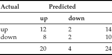
The table shows that the network predicts the upward movement well, but fares poorly in forecasting the downward movement of the stock. The chi-squared statistic of the table is 0.137 with 77-value 0.71. Consequently, the network does not significantly outperform a random-walk model with equal probabilities for “upward” and “downward” movements.
Magnitude Measure
Three statistics are commonly used to measure performance of point forecasts. They are the mean squared error (MSE), mean absolute deviation (MAD), and mean absolute percentage error (MAPE). For ℓ-step ahead forecasts, these measures are defined as
(49) ![]()
(50) ![]()
(51) ![]()
where m is the number of ℓ-step ahead forecasts available in the forecasting subsample.
In application, one often chooses one of the above three measures, and the model with the smallest magnitude on that measure is regarded as the best ℓ-step ahead forecasting model. It is possible that different ℓ may result in selecting different models. The measures also have other limitations in model comparison; see, for instance, Clements and Hendry (1993).
Distributional Measure
Practitioners recently began to assess forecasting performance of a model using its predictive distributions. Strictly speaking, a predictive distribution incorporates parameter uncertainty in forecasts. We call it conditional predictive distribution if the parameters are treated as fixed. The empirical distribution of xT+ℓ obtained by the parametric bootstrap is a conditional predictive distribution. This empirical distribution is often used to compute a distributional measure. Let uT(ℓ) be the percentile of the observed xT+ℓ in the prior empirical distribution. We then have a set of m percentiles ![]() , where again m is the number of ℓ-step ahead forecasts in the forecasting subsample. If the model entertained is adequate, {uT+j (ℓ)} should be a random sample from the uniform distribution on [0, 1]. For a sufficiently large m, one can compute the Kolmogorov-Smirnov statistic of {uT+j (ℓ)} with respect to uniform [0, 1]. The statistic can be used for both model checking and forecasting comparison.
, where again m is the number of ℓ-step ahead forecasts in the forecasting subsample. If the model entertained is adequate, {uT+j (ℓ)} should be a random sample from the uniform distribution on [0, 1]. For a sufficiently large m, one can compute the Kolmogorov-Smirnov statistic of {uT+j (ℓ)} with respect to uniform [0, 1]. The statistic can be used for both model checking and forecasting comparison.
2 APPLICATION
In this section, we illustrate nonlinear time series models by analyzing the quarterly U.S. civilian unemployment rate, seasonally adjusted, from 1948 to 1993. This series was analyzed in detail by Montgomery, Zarnowitz, Tsay, and Tiao (1998). We repeat some of the analyses here using nonlinear models. Figure 11 shows the time plot of the data. Well-known characteristics of the series include that (a) it tends to move countercyclically with U.S. business cycles, and (b) the rate rises quickly but decays slowly. The latter characteristic suggests that the dynamic structure of the series is nonlinear.
Figure 11 Time Plot of the U.S. Quarterly Unemployment Rate, Seasonally Adjusted, from 1948 to 1993
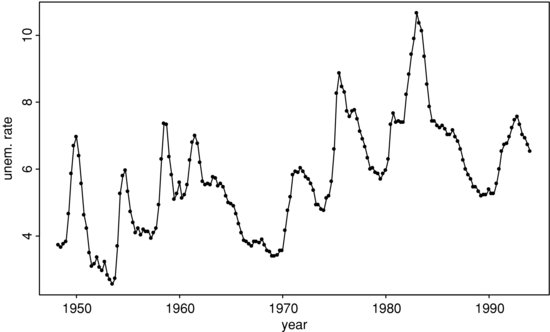
Denote the series by xt and let Δxt = xt−xt−1 be the change in unemployment rate. The linear model
was built by Montgomery et al. (1998), where the standard errors of the three coefficients are 0.11, 0.06, and 0.07, respectively. This is a seasonal model even though the data were seasonally adjusted. It indicates that the seasonal adjustment procedure used did not successfully remove the seasonality. This model is used as a benchmark model for forecasting comparison.
To test for nonlinearity, we apply some of the nonlinearity tests discussed earlier in this entry with an AR(5) model for the differenced series Δxt. The results are given in Table 3. All of the tests reject the linearity assumption. In fact, the linearity assumption is rejected for all AR(p) models we applied, where p = 2, … , 10.
Table 3 Nonlinearity Test for Changes in the U.S. Quarterly Unemployment Rate: 1948.II–1993.IV

Using a modeling procedure similar to that of Tsay (1989), Montgomery et al. (1998) build the following TAR model for the Δxt series:
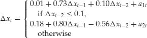
The sample variances of a1t and a2t are 0.76 and 0.165, respectively, the standard errors of the three coefficients of regime 1 are 0.03, 0.10, and 0.12, respectively, and those of regime 2 are 0.09, 0.1, and 0.16. This model says that the change in the U.S. quarterly unemployment rate, Δxt, behaves like a piecewise linear model in the reference space of xt−2 − xt−3 with threshold 0.1. Intuitively, the model implies that the dynamics of unemployment act differently depending on the recent change in the unemployment rate. In the first regime, the unemployment rate has had either a decrease or a minor increase. Here the economy should be stable, and essentially the change in the rate follows a simple AR(1) model because the lag-2 coefficient is insignificant. In the second regime, there is a substantial jump in the unemployment rate (0.1 or larger). This typically corresponds to the contraction phase in the business cycle. It is also the period during which government interventions and industrial restructuring are likely to occur. Here Δxt follows an AR(2) model with a positive constant, indicating an upward trend in xt. The AR(2) polynomial contains two complex characteristic roots, which indicate possible cyclical behavior in Δxt. Consequently, the chance of having a turning point in xt increases, suggesting that the period of large increases in xt should be short. This implies that the contraction phases in the U.S. economy tend to be shorter than the expansion phases.
Applying a Markov chain Monte Carlo method, Montgomery et al. (1998) obtain the following Markov switching model for Δxt:
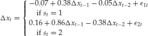
The conditional means of Δxt are −0.10 for st = 1 and 0.31 for st = 2. Thus, the first state represents the expansionary periods in the economy, and the second state represents the contractions. The sample variances of ![]() 1t and
1t and ![]() 2t are 0.031 and 0.192, respectively. The standard errors of the three parameters in state st = 1 are 0.03, 0.14, and 0.11, and those of state st = 2 are 0.04, 0.13, and 0.14, respectively. The state transition probabilities are P(st = 2|st−1 = 1) = 0.084(0.060) and P(st = 1|st−1 = 2) = 0.126(0.053), where the number in parentheses is the corresponding standard error. This model implies that in the second state the unemployment rate xt has an upward trend with an AR(2) polynomial possessing complex characteristic roots. This feature of the model is similar to the second regime of the TAR model in equation (53). In the first state, the unemployment rate xt has a slightly decreasing trend with a much weaker autoregressive structure.
2t are 0.031 and 0.192, respectively. The standard errors of the three parameters in state st = 1 are 0.03, 0.14, and 0.11, and those of state st = 2 are 0.04, 0.13, and 0.14, respectively. The state transition probabilities are P(st = 2|st−1 = 1) = 0.084(0.060) and P(st = 1|st−1 = 2) = 0.126(0.053), where the number in parentheses is the corresponding standard error. This model implies that in the second state the unemployment rate xt has an upward trend with an AR(2) polynomial possessing complex characteristic roots. This feature of the model is similar to the second regime of the TAR model in equation (53). In the first state, the unemployment rate xt has a slightly decreasing trend with a much weaker autoregressive structure.
Forecasting Performance
A rolling procedure was used by Montgomery et al. (1998) to forecast the unemployment rate xt. The procedure works as follows:
Table 4 shows the relative MSE of forecasts and mean forecast errors for the linear model in equation (52), the TAR model in equation (53), and the MSA model in equation (54), using the linear model as a benchmark. The comparisons are based on overall performance as well as the status of the U.S. economy at the forecast origin. From the table, we make the following observations:
Table 4 Out-of-Sample Forecast Comparison Among Linear, TAR, and MSA Models for the U.S. Quarterly Unemployment Rate
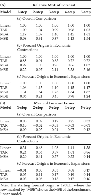
The results suggest that the contributions of nonlinear models over linear ones in forecasting the U.S. quarterly unemployment rate are mainly in the periods when the U.S. economy is in contraction. This is not surprising because, as mentioned before, it is during the economic contractions that government interventions and industrial restructuring are most likely to occur. These external events could introduce nonlinearity in the U.S. unemployment rate. Intuitively, such improvements are important because it is during the contractions that people pay more attention to economic forecasts.
KEY POINTS
- Nonlinearity exists in many financial data, including log returns of widely used market indexes such as CRSP equal- and value-weight indexes.
- Nonlinearity also appears in asset volatility. Indeed, simple threshold models such as the threshold GARCH model can be used to better describe the behavior of asset volatility. The model has been used to model the leverage effect between return and volatility.
- Simple nonparametric methods such as the local linear regression method can be used to provide a deeper understanding of interest rate dynamics.
- The unemployment rate example shows that, even though nonlinear models may not outperform linear ones in all forecast origins, they can provide more accurate forecasts when the U.S. economy is under contraction. This is useful because people in general pay more attention to forecasts during economic recession.
- Among the nonlinear models, the Markov switching model has the smallest bias in out-of-sample prediction. The model, however, has a larger mean square of forecast errors than the threshold autoregressive model. This behavior is consistent with the structure of the model because the true states of the economy are never certain under the switching model.
REFERENCES
Akaike, H. (1974). A new look at the statistical model identification. IEEE Transactions on Automatic Control AC-19: 716–723.
Andrews, D. W. K., and Ploberger, W. (1994). Optimal tests when a nuisance parameter is present only under the alternative. Econometrica 62: 1383–1414.
Box, G. E. P., Jenkins, G. M., and Reinsel, G. C. (2008). Time Series Analysis: Forecasting and Control, 4th ed. Hoboken, NJ: John Wiley.
Brock, W., Dechert, W. D., and Scheinkman, J. (1987). A test for independence based on the correlation dimension. Working paper, Department of Economics, University of Wisconsin, Madison.
Brock, W., Hsieh, D. A., and LeBaron, B. (1991). Nonlinear Dynamics, Chaos and Instability: Statistical Theory and Economic Evidence. Cambridge, MA: MIT Press.
Bryson, A. E., and Ho, Y. C. (1969). Applied Optimal Control. New York: Blaisdell.
Cai, Z., Fan, J., and Yao, Q. (2000). Functional-coefficient regression models for nonlinear time series. Journal of the American Statistical Association 95: 941–956.
Carlin, B. P., Polson, N. G., and Stoffer, D. S. (1992). A Monte Carlo approach to nonnormal and nonlinear state space modeling. Journal of the American Statistical Association 87: 493–500.
Chan, K. S. (1991). Percentage points of likelihood ratio tests for threshold autoregression. Journal of the Royal Statistical Society Series B 53: 691–696.
Chan, K. S. (1993). Consistency and limiting distribution of the least squares estimator of a threshold autoregressive model. The Annals of Statistics 21: 520–533.
Chan, K. S., and Tong H. (1986). On estimating thresholds in autoregressive models. Journal of Time Series Analysis 7: 179–190.
Chan, K. S., and Tsay, R. S. (1998). Limiting properties of the conditional least squares estimator of a continuous TAR model. Biometrika 85: 413–426.
Chen, C., McCulloch, R. E., and Tsay, R. S. (1997). A unified approach to estimating and modeling univariate linear and nonlinear time series. Statistica Sinica 7: 451–472.
Chen, R., and Tsay, R. S. (1991). On the ergodicity of TAR(1) processes. Annals of Applied Probability 1: 613–634.
Chen, R., and Tsay, R. S. (1993a). Functional-coefficient autoregressive models. Journal of the American Statistical Association 88: 298–308.
Chen, R., and Tsay, R. S. (1993b). Nonlinear additive ARX models. Journal of the American Statistical Association 88: 955–967.
Chen, R., Liu, J., and Tsay, R. S. (1995). Additivity tests for nonlinear autoregressive models. Biometrika 82: 369–383.
Chen, T., and Chen, H. (1995). Universal approximation to nonlinear operators by neural networks with arbitrary activation functions and its application to dynamical systems. IEEE Transactions on Neural Networks 6: 911–917.
Cheng, B., and Titterington, D. M. (1994). Neural networks: A review from a statistical perspective. Statistical Science 9: 2–54.
Clements, M. P., and Hendry, D. F. (1993). On the limitations of comparing mean square forecast errors. Journal of Forecasting 12: 617–637.
Cleveland, W. S. (1979). Robust locally weighted regression and smoothing scatterplots. Journal of the American Statistical Association 74: 829--836.
Creal, D., Koopman, S. J., and Lucas, A. (2010). Generalized autoregressive score models with applications. Working paper, Booth School of Business, University of Chicago.
Dahl, C. M., and Hylleberg, S. (1999). Specifying nonlinear econometric models by flexible regression models and relative forecast performance. Working paper, Department of Economics, University of Aarhus, Denmark.
Davis, R. B. (1987). Hypothesis testing when a nuisance parameter is present only under the alternative. Biometrika 74: 33–43.
Engle, R. F. (1982). Autoregressive conditional heteroscedasticity with estimates of the variance of United Kingdom inflations. Econometrica 50: 987–1007.
Epanechnikov, V. (1969). Nonparametric estimates of a multivariate probability density. Theory of Probability and Its Applications 14: 153–158.
Fan, J. (1993). Local linear regression smoother and their minimax efficiencies. The Annals of Statistics 21: 196–216.
Fan, J., and Yao, Q. (2003). Nonlinear Time Series: Nonparametric and Parametric Methods. New York: Springer-Verlag.
Gelfand, A. E., and Smith, A. F. M. (1990). Sampling-based approaches to calculating marginal densities. Journal of the American Statistical Association 85: 398–409.
Glosten, L. R., Jagannathan, R., and Runkle, D. E. (1993). On the relation between the expected value and the volatility of nominal excess return on stocks. Journal of Finance 48: 1779–1801.
Granger, C. W. J., and Andersen, A. P. (1978). An Introduction to Bilinear Time Series Models. Gottingen: Vandenhoek and Ruprecht.
Hamilton, J. D. (1989). A new approach to the economic analysis of nonstationary time series and the business cycle. Econometrica 57: 357–384.
Hamilton, J. D. (1990). Analysis of time series subject to changes in regime. Journal of Econometrics 45: 39–70.
Hamilton, J. D. (1994). Time Series Analysis. Princeton, NJ: Princeton University Press.
Härdle, W. (1990). Applied Nonparametric Regression. New York: Cambridge University Press.
Hansen, B. E. (1997). Inference in TAR models. Studies in Nonlinear Dynamics and Econometrics 1: 119–131.
Hinich, M. (1982). Testing for Gaussianity and linearity of a stationary time series. Journal of Time Series Analysis 3: 169–176.
Hornik, K. (1993). Some new results on neural network approximation. Neural Networks 6: 1069–1072.
Hornik, K., Stinchcombe, M., and White, H. (1989). Multilayer feedforward networks are universal approximators. Neural Networks 2: 359–366.
Hsieh, D. A. (1989). Testing for nonlinear dependence in daily foreign exchange rates. Journal of Business 62: 339–368.
Keenan, D. M. (1985). A Tukey non-additivity-type test for time series nonlinearity. Biometrika 72: 39–44.
Kitagawa, G. (1998). A self-organizing state space model. Journal of the American Statistical Association 93: 1203–1215.
Lewis, P. A. W., and Stevens, J. G. (1991). Nonlinear modeling of time series using multivariate adaptive regression spline (MARS). Journal of the American Statistical Association 86: 864–877.
Liu, J., and Brockwell, P. J. (1988). On the general bilinear time-series model. Journal of Applied Probability 25: 553–564.
Luukkonen, R., Saikkonen, P., and Teräsvirta, T. (1988). Testing linearity against smooth transition autoregressive models. Biometrika 75: 491–499.
McCulloch, R. E., and Tsay, R. S. (1993). Bayesian inference and prediction for mean and variance shifts in autoregressive time series. Journal of the American Statistical Association 88: 968–978.
McCulloch, R. E., and Tsay, R. S. (1994). Statistical inference of macroeconomic time series via Markov switching models. Journal of Time Series Analysis 15: 523–539.
McLeod, A. I., and Li, W. K. (1983). Diagnostic checking ARMA time series models using squared-residual autocorrelations. Journal of Time Series Analysis 4: 269–273.
Montgomery, A. L., Zarnowitz, V., Tsay, R. S., and Tiao, G. C. (1998). Forecasting the U. S. unemployment rate. Journal of the American Statistical Association 93: 478–493.
Nadaraya, E. A. (1964). On estimating regression. Theory and Probability Application 10: 186–190.
Petruccelli, J., and Woolford, S. W. (1984). A threshold AR(1) model. Journal of Applied Probability 21: 270–286.
Potter, S. M. (1995). A nonlinear approach to U.S. GNP. Journal of Applied Econometrics 10: 109–125.
Priestley, M. B. (1980). State-dependent models: A general approach to nonlinear time series analysis. Journal of Time Series Analysis 1: 47–71.
Priestley, M. B. (1988). Non-linear and Non-stationary Time Series Analysis. London: Academic Press.
Ramsey, J. B. (1969). Tests for specification errors in classical linear least squares regression analysis. Journal of the Royal Statistical Society Series B 31: 350–371.
Ripley, B. D. (1993). Statistical aspects of neural networks. In O. E. Barndorff-Nielsen, J. L. Jensen, and W. S. Kendall (eds.), Networks and Chaos—Statistical and Probablistic Aspects, pp. 40–123. London: Chapman and Hall.
Subba Rao, T., and Gabr, M. M. (1984). An introduction to bispectral analysis and bilinear time series models. Lecture Notes in Statistics, 24. New York: Springer-Verlag.
Teräsvirta, T. (1994). Specification, estimation, and evaluation of smooth transition autoregressive models. Journal of the American Statistical Association 89: 208–218.
Tiao, G. C., and Tsay, R. S. (1994). Some advances in nonlinear and adaptive modeling in time series. Journal of Forecasting 13: 109–131.
Tong, H. (1978). On a threshold model. In C. H. Chen (ed.), Pattern Recognition and Signal Processing. Amsterdam: Sijhoff & Noordhoff.
Tong, H. (1983). Threshold models in nonlinear time series analysis. Lecture Notes in Statistics. New York: Springer-Verlag.
Tong, H. (1990). Non-Linear Time Series: A Dynamical System Approach. Oxford: Oxford University Press.
Tsay, R. S. (1986). Nonlinearity tests for time series. Biometrika 73: 461–466.
Tsay, R. S. (1989). Testing and modeling threshold autoregressive processes. Journal of the American Statistical Association 84: 231–240.
Tsay, R. S. (1998). Testing and modeling multivariate threshold models. Journal of the American Statistical Association 93: 1188–1202.
Tsay, R. S. (2010). Analysis of Financial Time Series, 3rd ed. Hoboken, NJ: Wiley.
Venables, W. N., and Ripley, B. D. (1999). Modern Applied Statistics with S-Plus, 3rd ed. New York: Springer-Verlag.
Watson, G. S. (1964). Smooth regression analysis. Sankhya Series A 26: 359–372.