
Model Selection and Its Pitfalls
In this entry we discuss methods for model selection and analyze the many pitfalls of the model selection process.
MODEL SELECTION AND ESTIMATION
In his book Complexity, Mitchell Waldrop (1992) describes the 1987 Global Economy Workshop held at The Santa Fe Institute, a research center dedicated to the study of complex phenomena and related issues. Organized by the economist Bryan Arthur and attended by distinguished economists and physicists, the seminar introduced the idea that economic laws might be better understood applying the principles of physics and, in particular, the newly developed theory of complex systems. The seminar proceedings were to become the influential book The Economy as an Evolving Complex System (Anderson, Arrow, and Pines, 1998).
An anecdote from the book is revealing of the issues specific to economics as a scientific endeavor. According to Waldrop, physicists attending the seminar were surprised to learn that economists used highly sophisticated mathematics.
A physicist attending the seminar reportedly asked Kenneth Arrow, the 1972 Nobel Prize winner in economics, why, given the lack of data to support theories, economists use such sophisticated mathematics. Arrow replied, “It is just because we do not have enough data that we use sophisticated mathematics. We have to ensure the logical consistency of our arguments.” For physicists, on the other hand, explaining empirical data is the best guarantee of the logical consistency of theories. If theories work empirically, then mathematical details are not so important and will be amended later; if theories do not work empirically, no logical subtlety will improve them.
This anecdote is revealing of one of the key problems that any modeler of economic phenomena has to confront. On the one side, economics is an empirical science based on empirical facts. However, as data are scarce, many theories and models fit the same data. One is tempted to rely on “clear reasoning” to compensate for the scarcity of data. In economics, there is always a tension between the use of pure reasoning to develop ex ante economic theories and the need to conform to generally accepted principles of empirical science. The development of high-performance computing has aggravated the problem, making it possible to discover subtle patterns in data and to build models that fit data samples with arbitrary precision. But patterns and models selected in this way are meaningless and reveal no true economic feature.
Given the importance of model selection, let us discuss this issue before actually discussing estimation issues. It is perhaps useful to compare again the methods of economics and of physics. In physics, the process of model choice is largely based on human creativity. Facts and partial theories are accumulated until scientists make a major leap forward, discovering a new unifying theory. Theories are generally expressed through differential equations and often contain constants (i.e., numerical parameters) to be empirically ascertained. Note that the discovery of laws and the determination of constants are separate moments. Theories are often fully developed before the constants are determined; physical constants often survive major theoretical overhauls in the sense that new theories must include the same constants plus, eventually, additional ones.
Physicists are not concerned with problems of “data snooping,” that is, of fitting the data to the same sample that one wants to predict. In general, data are overabundant and models are not determined through a process of fitting and adaptation. Once a physical law that accurately fits all available data is discovered, scientists are confident that it will fit similar data in the future. The key point is that physical laws are known with a high level of precision. Centuries of theoretical thinking and empirical research have resulted in mathematical models that exhibit an amazing level of correspondence with reality. Any minor discrepancy from predictions to experiments entails a major scientific reevaluation. Often new laws have completely different forms but produce quite similar results. Experiments are devised to choose the winning theory.
Now consider economics, where the conceptual framework is totally different. First, though apparently many data are available, these data come in vastly different patterns. For example, the details of economic development are very different from year to year and from country to country. Asset prices seem to wander about in random ways. Introducing a concept that plays a fundamental role later in this entry, we can state: From the point of view of statistical estimation, economic data are always scarce given the complexity of their patterns.
Attempts to discover simple deterministic laws that accurately fit empirical economic data have proved futile. Furthermore, as economic data are the product of human artifacts, it is reasonable to believe that they will not follow the same laws for very long periods of time. Simply put, the structure of any economy changes too much over time to believe that economic laws are time-invariant laws of nature. One is, therefore, inclined to believe that only approximate laws can be discovered.
However the above considerations create an additional problem: The precise meaning of approximation must be defined. The usual response is to have recourse to probability theory. Here is the reasoning. Economic data are considered one realization of stochastic (i.e., random) data. In particular, economic time series are considered one realization of a stochastic process. The attention of the modeler has therefore to switch from discovering deterministic paths to determining the time evolution of probability distributions. In physics, this switch was made at the end of the 19th century, with the introduction of statistical physics. It later became an article of scientific faith that we can arrive at no better than a probabilistic description of nature.
The adoption of probability as a descriptive framework is not without a cost: Discovering probabilistic laws with confidence requires working with very large populations (or samples). In physics, this is not a problem as we have very large populations of particles. (Although this statement needs some qualification because physics has now reached the stage where it is possible to experiment with small numbers of elementary particles, it is sufficient for our discussion here.) In economics, however, populations are too small to allow for a safe estimate of probability laws; small changes in the sample induce changes in the laws. We can, therefore, make the following statement: Economic data are too scarce to allow us to make sure probability estimates.
For example, Gopikrishnan, Meyer, Nunes Amaral, and Stanley (1998) conducted a study to determine the distribution of stock returns at short time horizons, from a few minutes to a few days. They found that returns had a power tail distribution with exponent α ≈ 3. One would expect that the same measurement repeated several times over would give the same result. But this is not the case. Since the publication of the aforementioned paper, the return distribution has been estimated several times, obtaining vastly different results. Each successive measurement was made in bona fide, but a slightly different empirical setting produced different results.
As a result of the scarcity of economic data, many statistical models, even simple ones, can be compatible with the same data with roughly the same level of statistical confidence. For example, if we consider stock price processes, many statistical models—including the random walk—compete to describe each process with the same level of significance. Before discussing the many issues surrounding model selection and estimation, we will briefly discuss the subject of machine learning and the machine-learning approach to modeling.
THE (MACHINE) LEARNING APPROACH TO MODEL SELECTION
There is a fundamental distinction between (1) estimating parameters in a well-defined model and (2) estimating models through a process of learning. Models, as mentioned, are determined by human modelers using their creativity. For example, a modeler might decide that stock returns in a given market are influenced by a set of economic variables and then write a linear model as follows:
![]()
where the f are stochastic processes that represent a set of given economic variables. The modeler must then estimate the βk and test the validity of his model.
In the machine-learning approach to modeling—ultimately a byproduct of the diffusion of computers—the process is the following:
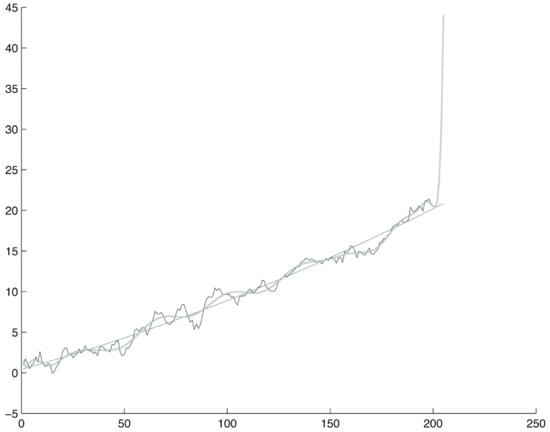
Figure 1 Polynomial Fitting of a Trend Stationary Process Using Two Polynomials of Degree 2 and 20 Respectively on a Training Window of 200 Steps
- There is a set of empirical data to explain.
- Data are explained by a family of models that include an unbounded number of parameters.
- Models fit with arbitrary precision any set of data.
That models can fit any given set of data with arbitrary precision is illustrated by neural networks, one of the many machine learning tools used to model data that includes genetic algorithms. As first demonstrated by Cybenko (1989), neural networks are universal function approximators. If we allow a sufficient number of layers and nodes, a neural network can approximate any given function with arbitrary precision. The idea of universal function approximators is well known in calculus. The Taylor and Fourier series are universal approximators for broad classes of functions.
Suppose a modeler wants to model the unknown data generation process (DGP) of a time series X(t) using a neural network. A DGP is a possibly nonlinear function of the following type:
![]()
that links the present value of the series to its past. A neural network will try to learn the function F using empirical data from the series. If the number of layers and nodes is not constrained, the network can learn F with unlimited precision.
However, the key concept of the theory of machine learning is that a model that can fit any data set with arbitrary precision has no explanatory power, that is, it does not capture any true feature of the data, neither in a deterministic setting nor in a statistical setting. In an economic context, machine learning perfectly explains sample data but has no forecasting power. It is only a mathematical device; it does not correspond to any economic property.
We can illustrate this point in a simplified setting. Let us generate an autoregressive trend stationary process according to the following model:
![]()
where ε(i) are normally distributed zero-mean unit-variance random numbers generated with a random number generator. The initial condition is X = 1. This process is asymptotically trend stationary. Using the ordinary least squares (OLS) method, let us fit to the process X two polynomials of degree 2 and 20 respectively on a training window of 200 steps. We continue the polynomials five steps after the training window. Figure 1 represents the process plot and the two polynomials. Observe from the exhibit the different behavior of the two polynomials. The polynomial of degree 2 essentially repeats the linear trend, while the polynomial of degree 20 follows the random fluctuations of the process quite accurately. Immediately after, however, the training window it diverges.
To address the problem, the theory of machine learning suggests criteria to constrain models so that they fit sample data only partially but, as a trade-off, retain some forecasting power. The intuitive meaning is the following: The structure of the data and the sample size dictate the complexity of the laws that can be learned by computer algorithms.
This is a fundamental point. If we have only a small sample data set we can learn only simple patterns, provided that these patterns indeed exist. The theory of machine learning constrains the dimensionality of models to make them adapt to the sample size and structure.
In most practical applications, the theory of machine learning works by introducing a penalty function that constrains the models. The penalty function is a function of the size of the sample and of the complexity of the model. One compares models by adding the penalty function to the likelihood function (a definition of the likelihood function is provided later). In this way one can obtain an ideal trade-off between model complexity and forecasting ability.
Several proposals have been made as regards the shape of the penalty function. Three criteria are in general use:
- The Akaike Information Criterion (AIC)
- The Bayesian Information Criterion (BIC) of Schwartz
- The Maximum Description Length principle of Rissanen
More recently, Vapnik and Chervonenkis (1974) have developed a full-fledged quantitative theory of machine learning. While this theory goes well beyond the scope of this book, the practical implication of the theory of learning is important to note: Model complexity must be constrained in function of the sample.
Consider that some “learning” appears in most financial econometric endeavors. For example, determining the number of lags in an autoregressive model is a problem typically solved with methods of learning theory, that is, by selecting the number of lags that minimize the sum of the loss function of the model plus a penalty function. Ultimately, in modern computer-based financial econometrics, there is no clear-cut distinction between a learning approach versus a theory-based a priori approach.
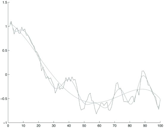
Note, however, that the theory of machine learning offers no guarantee of success. To see this point, let’s generate a random walk and fit two polynomials of degree 3 and 20, respectively. Figure 2 illustrates the random path and the two polynomials. The two polynomials appear to fit the random path quite well. Following the above discussion, the polynomial of order 3 seems to capture some real behavior of the data. But as the data are random, the fit is spurious. This is by no means a special case. In general, it is often possible to fit models to sample data even if the data are basically unpredictable.
Figure 2 Polynomial Fitting of a Random Walk Using Two Polynomials of Degree 3 and 20 Respectively on a 100-Step Sample
Figures 1 and 2 are examples of the simplest cases of model fitting. One might be tempted to object that fitting a curve with a polynomial is not a good modeling strategy for prices or returns. This is true, as one should model a dynamic DGP. However, fitting a DGP implies a multivariate curve fitting. For illustration purposes, we chose the polynomial fitting of a univariate curve: It is easy to visualize and contains all the essential elements of model fitting.
SAMPLE SIZE AND MODEL COMPLEXITY
The four key conclusions reached thus far are
- Economic data are generally scarce for statistical estimation given the complexity of their patterns.
- Economic data are too scarce for sure statistical estimates.
- The scarcity of data means that the data might be compatible with many different models.
- There is a trade-off between model complexity and the size of the data sample.
The last two considerations are critical. To illustrate the quantitative trade-off between the size of a data sample and model complexity, consider an apparently straightforward case: estimating a correlation matrix.
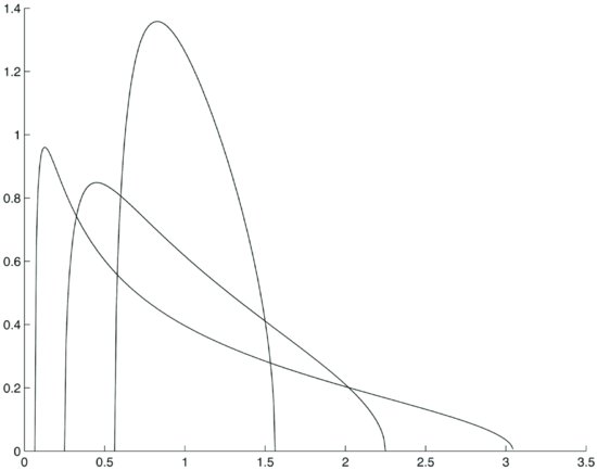
It is well known from the theory of random matrices that the eigenvalues of the correlation matrix of independent random walks are distributed according to the following law:
![]()
where Q is the ratio between the number N of sample points and the number M of time series. Figure 3 illustrates the theoretical distribution of eigenvalues for three values of Q: Q = 1.8, Q = 4, and Q = 16.
As can be easily predicted by examining the above formula, the distribution of eigenvalues is broader when Q is smaller. The corresponding λmax is larger for the broader distribution. The λmax are respectively:
The eigenvalues of a random matrix do not carry any true correlation information. If we now compute the eigenvalues of an empirical correlation matrix of asset returns with a given Q (i.e., the ratio between number of samples and the number of series), we find that only a few eigenvalues carry information as they are outside the area of pure randomness corresponding to the Q. In fact, with good approximation, λmax is the cut-off point that separates meaningful correlation information from noise. (The application of random matrices to the estimation of correlation and covariance matrices is developed in Plerou, Gopikrishnan, Rosenow, Nunes Amaral, Guhr, and Stanley [2002].) Therefore, as the ratio of sample points to the number of asset prices grows (i.e., we have more points for each price process) the “noise area” gets smaller.
Figure 3 The Theoretical Distribution of Eigenvalues for Three Values of Q: Q = 1.8, Q = 4, and Q = 16
To show the effects of the ratio Q on the estimation of empirical correlation matrices, let’s compute the correlation matrix for three sets of 900, 400, and 100 stock prices that appeared in the MSCI Europe in a six-year period from December 1998 to February 2005. The return series contain in total 1,611 sample points, each corresponding to a trading day.
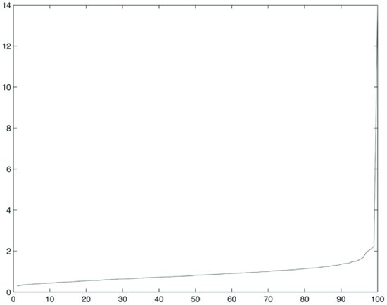
First we compute the correlation matrices. The average correlation (excluding the diagonal) is approximately 10% for the three sets of 100, 400, and 900 stocks. Then we compute the eigenvalues. The plot of sorted eigenvalues for the three samples is shown in Figures 4, 5, and 6. One can see from these exhibits that when the ratio Q is equal to 16 (i.e., we have more sample points per stock price process), the plot of eigenvalues decays more slowly.
Figure 4 Plot of Eigenvalues for 900 Prices, Q = 1.8
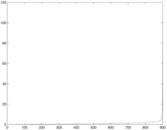
Figure 5 Plot of Eigenvalues for 400 Prices, Q = 4
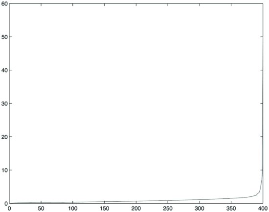
Figure 6 Plot of Eigenvalues for 100 Prices, Q = 16
Now compare the distribution of empirical eigenvalues with the theoretical cut-off point λmax that we computed above. The parameter Q was chosen to approximately represent the ratios between 1,611 sample points and 100, 400, and 900 stocks. Results are tabulated in Table 1. This exhibit shows that the percentage of meaningful eigenvalues grows as the ratio between the number of sample points and the number of processes increases. If we hold the number of sample points constant (i.e., 1,611) and increase the number of time series from 100 to 900, a larger percentage of eigenvalues becomes essentially noise (i.e., they do not carry information). Obviously the number of meaningful eigenvalues increases with the number of series, but, due to loss of information, it does so more slowly than does the number of series due to loss of information.
Table 1 Comparison of the Distribution of Empirical Eigenvalues with the Theoretical Cutoff Point for Different Values of Q
Two main conclusions can be drawn from Table 1:
- Meaningful eigenvalues represent a small percentage of the total, even when Q = 16.
- The ratio of meaningful eigenvalues to the total grows with Q, but the gain is not linear.
The above considerations apply to estimating a correlation matrix. As we will see, however, they carry over, at least qualitatively, to the estimation of any linear dynamic model. In fact, the estimation of linear dynamic models is based on estimating correlation and covariance matrices.
DANGEROUS PATTERNS OF BEHAVIOR
One of the most serious mistakes that a financial modeler can make is to look for rare or unique patterns that look profitable in-sample but produce losses out-of-sample. This mistake is made easy by the availability of powerful computers that can explore large amounts of data: Any large data set contains a huge number of patterns, many of which look very profitable. Otherwise expressed, any large set of data, even if randomly generated, can be represented by models that appear to produce large profits. To see the point, perform the following simple experiment. Using a good random number generator, generate a large number of independent random walks with zero drift. In sample, these random walks exhibit large profit opportunities. There are numerous reasons for this. In fact, if we perform a sufficiently large number of simulations, we will generate a number of paths that are arbitrarily close to any path we want. Many paths will look autocorrelated and will be indistinguishable from trend-stationary processes. In addition, many stochastic trends will be indistinguishable from deterministic drifts.
There is nothing surprising in the above phenomena. A stochastic process or a discrete time series is formed by all possible paths. For example, a trend-stationary process and a random walk are formed by the same paths. What makes the difference between a trend-stationary process and a random walk are not the paths—which are exactly the same—but the probability assignments. Suppose processes are discrete, for example because time is discrete and prices move by only discrete amounts. Any computer simulation is ultimately a discrete process, though the granularity of the process is very small. In this discrete case, we can assign a discrete probability to each path. The difference between processes is the probability assigned to each path. In a large sample, even low probability paths will occur, albeit in small numbers.
In a very large data set, almost any path will be approximated by some path in the sample. If the computer generates a sufficiently large number of random paths, we will come arbitrarily close to any given path, including, for example, to any path that passes the test for trend stationarity. In any large set of price processes, one will therefore always find numerous interesting paths, such as cointegrated pairs and trend-stationary processes.
To avoid looking for ephemeral patterns, we must stick rigorously to the paradigm of machine learning and statistical tests. This sounds conceptually simple, but it is very difficult to do in practice. It means that we have to decide the level of confidence that we find acceptable and then compute probability distributions for the entire sample. This has somewhat counterintuitive consequences. We illustrate this point using as an example the search for cointegrated pairs; the same reasoning applies to any statistical property.
Suppose that we have to decide whether a given pair of time series is cointegrated or not. We can use one of the many cointegration tests. If the time series are short, no test will be convincing; the longer the time series, the more convincing the test. The problem with economic data is that no test is really convincing as the confidence level is generally in the range of 95% or 99%. Whatever confidence level we choose, given one or a small number of pairs, we decide the cointegration properties of each pair individually. For example, in macroeconomic studies where only a few time series are given, we decide if a given pair of time series is cointegrated or not by looking at the cointegration test for that pair.
Does having a large number of data series, for example 500 price time series, require any change in the testing methodology? The answer, in fact, is that additional care is required: In a large data set, for the reasons we outlined above, any pattern can be approximated. One has to look at the probability that a pattern will appear in that data set. In the example of cointegration, if one finds, say, ten cointegrated pairs in 500 time series, the question to ask is: What is the probability that in 500 time series 10 time series are cointegrated? Answering this question is not easy because the properties of pairs are not independent. In fact, given three series a, b, and c we can form three distinct pairs whose cointegration properties are not, however, mutually independent. This makes calculations difficult.
To illustrate the above, let us generate a simulated random walk using the following formula:
![]()
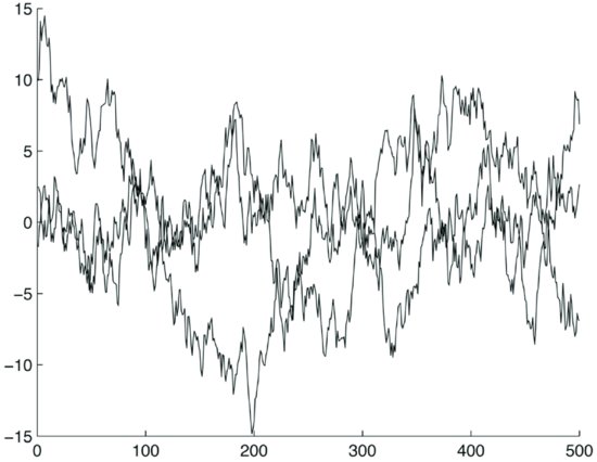
where X(i) is a random vector with 500 elements, and the noise term is generated with a random number generator as 500 independent normally distributed zero-mean unitary-variance numbers. Now run simulations for 500 steps. Next, eliminate linear trends from each realization. (Cointegration tests can handle linear trends. We detrended for clarity of illustrations.) A sample of three typical realizations of the random walks is illustrated in Figure 7 and the corresponding residuals after detrending in Figure 8.
Figure 7 A Sample of Three Typical Realizations of a 500-Step Random Walk with Their Trends
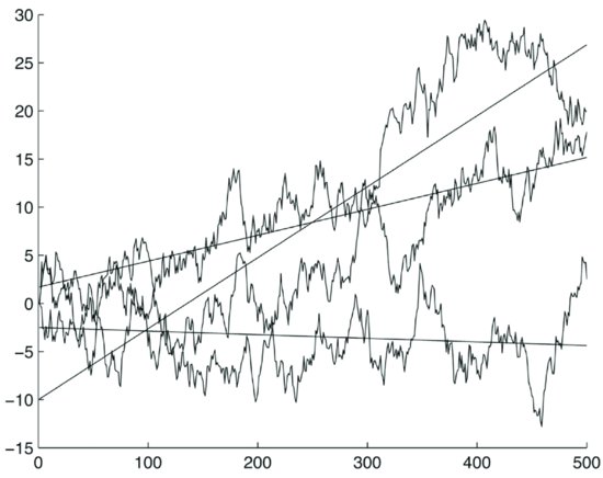
Figure 8 The Residuals of the Same Random Walks after Detrending
Now run the cointegration test at a 99% confidence level on each possible pair. In a sample of 10 simulation runs, we obtain the following number of pairs that pass the cointegration test: 74, 75, 89, 73, 65, 91, 91, 93, 84, 62. There are in total
![]()
If cointegration properties of pairs were independent, given 500 random walks, on the average we should find 124 pairs that pass the cointegration test at the 99% confidence level. However, cointegration properties of pairs are not independent for the reasons mentioned above. This explains why we obtained a smaller number of pairs than expected. This example illustrates the usefulness of running Monte Carlo experiments to determine the number of cointegrated pairs found in random walks.
If, however, the patterns we are looking for are all independent, calculations are relatively straightforward. Suppose we are looking for stationary series applying an appropriate test at a 99% confidence interval. This means that a sample random walk has a 1% probability of passing the test (i.e., to be wrongly accepted as stationary) and a 99% probability of being correctly rejected. In this case, the probability distribution of the number of paths that pass the stationarity test given a sample of 500 generated random walks is a binomial distribution with probabilities p = 0.01 and q = 1 − p = 0.99 and mean 5.
We apply criteria of this type very often in our professional and private lives. For example, suppose that an inspector has to decide whether to accept or reject a supply of spare parts. The inspector knows that on average one part in 100 is defective. He randomly chooses a part in a lot of 100 parts. If the part is defective, he is likely to ask for additional tests before accepting the lot. Suppose now that he tests 100 parts from 100 different lots of 100 parts and finds only one defective part. He is likely to accept the 100 lots because the incidence of faulty parts is what he expected it to be, that is, one in 100. The point is that we are looking for statistical properties, not real identifiable objects.
A profitable price time series is not a recognizable object. We find what seems to be a profitable time series but we cannot draw any conclusion because the level of the “authenticity test” of each series is low. When looking at very large data sets, we have to make data work for us and not against us, examining the entire sample. For example, consider a strategy known as “pair trading.” In this strategy, an investor selects pairs from a stock universe and maintains a market neutral (i.e., zero beta) long-short portfolio of several pairs of stocks with a mean-reverting spread. When there are imbalances in the market causing the spread to diverge, the investor seeks to determine the reason for the divergence. If the investor believes that the spread will revert, he or she takes a position in the two stocks to capitalize on the reversion. A modeler who would define a pair trading strategy based on the cointegrated pair in the previous example would be disappointed. Based on extensive Monte Carlo simulations to compare the number of cointegrated pairs among the stocks in the S&P 500 index for the period 2001–2004 and in computer-generated random walks, the number of cointegrated pairs we found was slightly larger in the real series than in the simulated random walks.
We can conclude that it is always good practice is to test any model or pattern recognition method against a surrogated random sample generated with the same statistical characteristics as the empirical ones. For example, it is always good practice to test any model and any strategy intended to find excess returns on a set of computer-generated random walks. If the proposed strategy finds profit in computer-generated random walks, it is highly advisable to rethink the strategy.
DATA SNOOPING
Given the scarcity of data and the basically uncertain nature of any econometric model, it is generally required to calibrate models on some data set, the so-called training set, and test them on another data set, the test set. In other words, it is necessary to perform an out-of-sample validation on a separate test set. The rationale for this procedure is that any machine-learning process—or even the calibration mechanism itself—is a heuristic methodology, not a true discovery process. Models determined through a machine-learning process must be checked against the reality of out-of-sample validation. Failure to do so is referred to as data snooping, that is, performing training and tests on the same data set.
Out-of-sample validation is typical of machine-learning methods. Learning entails models with unbounded capabilities of approximation constrained by somewhat artificial mechanisms such as a penalty function. This learning mechanism is often effective but there is no guarantee that it will produce a good model. Therefore, the learning process is considered discovery heuristics. The true validation test, say the experiments, has to be performed on the test set. Needless to say, the test set must be large and cover all possible patterns, at least in some approximate sense. For example, in order to test a trading strategy one would need to test data in many different market conditions: with high volatility and low volatility, in expansionary and recessionary economic periods, under different correlation situations, and so on.
Data snooping is not always easy to understand or detect. Suppose that a modeler wants to build the DGP of a time series. A DGP is often embodied in a set of difference equations with parameters to be estimated. Suppose that four years of data of a set of time series are available. A modeler might be tempted to use the entire four years to perform a “robust” model calibration and to “test” the model on the last year. This is an example of data snooping that might be difficult to recognize and to avoid. In fact, one might (erroneously) reason as follows. If there is a true DGP, it is more likely that it is “discovered” on a four-year sample than on shorter samples. If there is a true DGP, data snooping is basically innocuous and it is therefore correct to use the entire data set. On the other hand, if there is no stable DGP, then it does not make sense to calibrate models as their coefficients would be basically noise.
This reasoning is wrong. In general, there is no guarantee that, even if a true DGP exists, a learning algorithm will learn it. Among the reasons for learning failure are (1) the slow convergence of algorithms which might require more data than that available, and (2) the possibility of getting stuck in local optima. However, the real danger is the possibility that no true DGP exists. Should this be the case, the learning algorithm might converge to a false solution or not converge at all. We illustrated this fact earlier in this entry where we showed how it is possible to successfully fit a low dimensionality polynomial to a randomly generated path.
There are other forms of data snooping. Suppose that a modeling team works on a sample of stock price data to find a profitable trading strategy. Suppose that they respect all of the above criteria of separation of the training set and the data set. Different strategies are tried and those that do not perform are rejected. Though sound criteria are used, there is still the possibility that by trial and error the team hits a strategy that performs well in sample but poorly when applied in the real world. Another form of hidden data snooping is when a methodology is finely calibrated to sample data. Again, there is the possibility that by trial and error one finds a calibration parameterization that works well in sample and poorly in the real world.
There is no sound theoretical way to avoid this problem ex ante. In practice, the answer is to separate the sets of training data and test data, and to decide on the existence of a DGP in function of performance on the test data. However, this type of procedure requires a lot of data. “Resampling” techniques have been proposed to alleviate the problem. Intuitively, the idea behind resampling methods is that a stable DGP calibrated on any portion of the data should work on the remaining data. Widely used resampling techniques include “leave-one-out” and “bootstrapping.” The bootstrap technique creates surrogated data from the initial sample data. (The bootstrap is an important technique but its description goes beyond the scope of this entry. For a review of bootstrapping, see Davison and Hinkley [1997].)
Data snooping is a defect of training processes which must be controlled but which is very difficult to avoid given the size of data samples currently available. Suppose samples in the range of ten years are available. (Technically much longer data sets on financial markets, up to 50 years of price data, are available. While useful for some applications, these data are useless for most asset management applications given the changes in the structure of the economy.) One can partition these data and perform a single test free from data snooping biases. However, if the test fails, one has to start all over again and design a new strategy. The process of redesigning the modeling strategy might have to be repeated several times over before an acceptable solution is found. Inevitably, repeating the process on the same data includes the risk of data snooping. The real danger in data snooping is the possibility that by trial and error or by optimization, one hits upon a model that casually performs well on the sample data but that will perform poorly in real-world forecasts. Fabozzi, Focardi, and Ma (2005) explore at length different ways in which data snooping and other biases might enter the model discovery process and propose a methodology to minimize the risk of biases, as will be explained in the last section of this entry.
SURVIVORSHIP BIASES AND OTHER SAMPLE DEFECTS
We now examine possible defects of the sample data themselves. In addition to errors and missing data, one of the most common (and dangerous) defects of sample data are the so-called survivorship biases. The survivorship bias is a consequence of selecting time series, in particular asset price time series, based on criteria that apply at the end of the period. For example, suppose a sample contains 10 years of price data for all stocks that are in the S&P 500 today and that existed for the last 10 years. This sample, apparently well formed, is, however, biased: The selection, in fact, is made on the stocks of companies that are in the S&P 500 today, that is, those companies that have “survived” in sufficiently good shape to still be in the S&P 500 aggregate. The bias comes from the fact that many of the surviving companies successfully passed through some difficult period. Surviving the difficulty is a form of reversion to the mean that produces trading profits. However, at the moment of the crisis it was impossible to predict which companies in difficulty would indeed have survived.
To gauge the importance of the survivorship bias, consider a strategy that goes short on a fraction of the assets with the highest price and long on the corresponding fraction with the lowest price. This strategy might appear highly profitable in sample. Looking at the behavior of this strategy, however, it becomes clear that profits are very large in the central region of the sample and disappear approaching the present day. This behavior should raise flags. Although any valid trading strategy will have good and bad periods, profit reduction when approaching the present day should command heightened attention.
Avoiding the survivorship bias seems simple in principle: It might seem sufficient to base any sample selection at the moment where the forecast begins, so that no invalid information enters the strategy prior to trading. However, the fact that companies are founded, merged, and closed plays havoc with simple models. In fact, calibrating a simple model requires data of assets that exist over the entire training period. This in itself introduces a potentially substantial training bias.
A simple model cannot handle processes that start or end in the middle of the training period. On the other hand, models that take into account the foundation or closing of firms cannot be simple. Consider, for example, a simple linear autoregressive model. Any addition or deletion of companies introduces a nonlinearity in the model and precludes using standard tools such as the OLS method.
There is no ideal solution. Care is required in estimating possible performance biases consequent to sample biases. Suppose that we make a forecast of return processes based on models trained on the past three or four years of returns data on the same processes that we want to forecast. Clearly there is no data snooping, as we use only information available prior to forecasting. However, it should be understood that we are estimating our models on data that contain biases. If the selection of companies to forecast is subject to strong criteria, for example companies that belong to a major index, it is likely that the model will suffer a loss of performance. This is due to the fact that models will be trained on spurious past performance. If the modeler is constrained to work on a specific stock selection, for example because he has to create an active strategy against a selected benchmark, he might want to consider Bayesian techniques to reduce the biases.
The survivorship bias is not the only possible bias of sample data. More in general, any selection of data contains some bias. Some of these biases are intentional. For example, selecting large caps or small caps introduces special behavioral biases that are intentional. However, other selection biases are more difficult to appreciate. In general, any selection based on belonging to indexes introduces index-specific biases in addition to the survivorship bias. Consider that presently thousands of indexes are in use—the FTSE alone has created some 60,000. Institutional investors and their consultants use these indexes to create asset allocation strategies and then give the indexes to asset managers for active management.
Anyone creating active management strategies based on these indexes should be aware of the biases inherent in the indexes when building their strategies. Data snooping applied to carefully crafted stock selection can result in poor performance because the asset selection process inherent in the index formation process can produce very good results in sample; these results vanish out-of-sample as “snow under the sun.”
MOVING TRAINING WINDOWS
Thus far we assumed that the DGP exists as a time-invariant model. Can we also assume that the DGP varies and that it can be estimated on a moving window? If yes, how can it be tested? These are complex questions that do not admit an easy answer. It is often assumed that the economy undergoes “structural breaks” or “regime shifts” (i.e., that the economy undergoes discrete changes at fixed or random time points).
If the economy is indeed subject to breaks or shifts and the time between breaks is long, models would perform well for a while and then, at the point of the break, performance would degrade until a new model is learned. If regime changes are frequent and the interval between the changes short, one could use a model that includes the changes. The result is typically a nonlinear model such as the Markov-switching models. Estimating models of this type is very onerous given the nonlinearities inherent in the model and the long training period required.
There is, however, another possibility that is common in modeling. Consider a model that has a defined structure, for example a linear VAR model, but whose coefficients are allowed to change in time with the moving of the training window. In practice, most models used work in this way as they are periodically recalibrated. The rationale of this strategy is that models are assumed to be approximate and sufficiently stable for only short periods of time. Clearly there is a trade-off between the advantage of using long training sets and the disadvantage that a long training set includes too much change.
Intuitively, if model coefficients change rapidly, this means that the model coefficients are noisy and do not carry genuine information. We have seen an example above in the simple case of estimating a correlation matrix. Therefore, it is not sufficient to simply reestimate the model: One must determine how to separate the noise from the information in the coefficients. For example, a large VAR model used to represent prices or returns will generally be unstable. It would not make sense to reestimate the model frequently; one should first reduce model dimensionality with, for example, factor analysis. Once model dimensionality has been reduced, coefficients should change slowly. If they continue to change rapidly, the model structure cannot be considered appropriate. One might, for example, have ignored fat tails or essential nonlinearities.
How can we quantitatively estimate an acceptable rate of change for model coefficients? Are we introducing a special form of data snooping in calibrating the training window? Clearly the answer depends on the nature of the true DGP—assuming that one exists. It is easy to construct artificially DGPs that change slowly in time so that the learning process can progressively adapt to them. It is also easy to construct true DGPs that will play havoc with any method based on a moving training window. For example, if one constructs a linear model where coefficients change systematically at a frequency comparable with a minimum training window, it will not be possible to estimate the process as a linear model estimated on a moving window.
Calibrating a training window is clearly an empirical question. However, it is easy to see that calibration can introduce a subtle form of data snooping. Suppose a rather long set of time series is given, say six to eight years, and that one selects a family of models to capture the DGP of the series and to build an investment strategy. Testing the strategy calls for calibrating a moving window. Different moving windows are tested. Even if training and test data are kept separate so that forecasts are never performed on the training data, clearly the methodology is tested on the same data on which the models are learned.
Other problems with data snooping stem from the psychology of modeling. A key precept that helps to avoid biases is the following: Modeling hunches should be based on theoretical reasoning and not on looking at the data. This statement might seem inimical to an empirical enterprise, an example of the danger of “clear reasoning” mentioned above. Still, it is true that by looking at data too long one might develop hunches that are sample-specific. There is some tension between looking at empirical data to discover how they behave and avoiding to capture the idiosyncratic behavior of the available data.
In his best-seller Chaos: Making a New Science, James Gleick (1987) reports that one of the initiators of chaos theory used to spend long hours flying planes (at his own expense) just to contemplate clouds to develop a feeling for their chaotic movement. Obviously there is no danger of data snooping in this case as there are plenty of clouds on which any modeling idea can be tested. In other cases, important discoveries have been made working on relatively small data samples. The 20th-century English hydrologist Harold Hurst developed his ideas of rescaled range analysis from the yearly behavior of the Nile River, approximately 500 years of sample data, not a huge data sample.
Clearly simplicity (i.e., having only a small number of parameters to calibrate) is a virtue in modeling. A simple model that works well should be favored over a complex model that might produce unpredictable results. Nonlinear models in particular are always subject to the danger of unpredictable chaotic behavior. It was a surprising discovery that even simple maps originate highly complex behavior. The conclusion is that every step of the discovery process has to be checked for empirical, theoretical, and logical consistency.
MODEL RISK
As we have seen above, any model choice and estimation process might result in biases and poor performance. In other words, any model selection process is subject to model risk. One might well ask if it is possible to mitigate model risk. In statistics, there is a long tradition, initiated by the 18th-century English mathematician Thomas Bayes, of considering uncertain not only individual outcomes but the probability distribution itself. It is therefore natural to see if ideas from Bayesian statistics and related concepts could be applied to mitigate model risk.
A simple idea that is widely used in practice is to take the average of different models. This idea can take different forms. Suppose that we have to estimate a variance-covariance matrix. It makes sense to take radically different estimates such as noisy empirical estimates and capital asset pricing model (CAPM) estimates that only consider covariances with the market portfolio and average. Averaging is done with the principle of shrinkage, that is, one does not form a pure average but weights the two matrices with weights a and 1 − a, choosing a according to some optimality principle. This idea can be extended to dynamic models, weighting all coefficients in a model with a probability distribution. Here we want to make some additional qualitative considerations that lead to strategies in model selection.
There are two principal reasons for applying model risk mitigation. First, we might be uncertain as to which model is best, and so mitigate risk by diversification. Second, perhaps more cogent, we might believe that different models will perform differently under different circumstances. By averaging, we hope to reduce the volatility of our forecasts. It should be clear that averaging model results or working to produce an average model (i.e., averaging coefficients) are two different techniques. The level of difficulty involved is also different.
Averaging results is a simple matter. One estimates different models with different techniques, makes forecasts and then averages the forecasts. This simple idea can be extended to different contexts. For example, in rating stocks one might want to do an exponential averaging over past ratings, so that the proposed rating today is an exponential average of the model rating today and model ratings in the past. Obviously parameters must be set correctly, which again forces a careful analysis of possible data snooping biases. Whatever the averaging process one uses, the methodology should be carefully checked for statistical consistency. For example, one obtains quite different results applying methodologies based on averaging to stationary or nonstationary processes. The key principle is that averaging is used to eliminate noise, not genuine information.
Averaging models is more difficult than averaging results. In this case, the final result is a single model, which is, in a sense, the average of other models. Shrinkage of the covariance matrix is a simple example of averaging models.
MODEL SELECTION IN A NUTSHELL
It is now time to turn all the caveats into some positive approach to model selection. As remarked in Fabozzi, Focardi, and Ma (2005), any process of model selection must start with strong economic intuition. Data mining and machine learning alone are unlikely to produce significant positive results. The possibility that scientific discovery, and any creative process in general, can be “outsourced” to computers is still far from today’s technological reality. A number of experimental artificial intelligence (AI) programs have indeed shown the ability to “discover” scientific laws. For example, the program KAM developed by Yip (1989) is able to analyze nonlinear dynamic patterns and the program TETRAD developed at Carnegie Mellon is able to discover causal relationships in data (see Glymour, Scheines, Spirtes, and Kelly, 1987). However, practical applications of machine intelligence use AI as a tool to help perform specific tasks.
Economic intuition clearly entails an element of human creativity. As in any other scientific and technological endeavor, it is inherently dependent on individual abilities. Is there a body of true, shared science that any modeler can use? Or do modelers have to content themselves with only partial and uncertain findings reported in the literature? As of the writing of this book, the answer is probably a bit of both.
One would have a hard time identifying economic laws that have the status of true scientific laws. Principles such as the absence of arbitrage are probably what comes closest to a true scientific law but are not, per se, very useful in finding, say, profitable trading strategies. Most economic findings are of an uncertain nature and are conditional on the structure of the economy or the markets.
It is fair to say that economic intuition is based on a number of broad economic principles plus a set of findings of an uncertain and local nature. Economic findings are statistically validated on a limited sample and probably hold only for a finite time span. Consider, for example, findings such as volatility clustering. One might claim that volatility clustering is ubiquitous and that it holds for every market. In a broad sense this is true. However, no volatility clustering model can claim the status of a law of nature as all volatility clustering models fail to explain some essential fact.
It is often argued that profitable investment strategies can be based only on secret proprietary discoveries. This is probably true but its importance should not be exaggerated. Secrecy is typically inimical to knowledge building. Secrets are also difficult to keep. Historically, the largest secret knowledge-building endeavors were related to military efforts. Some of these efforts were truly gigantic, such as the Manhattan Project to develop the first atomic bomb. Industrial projects of a non-military nature are rarely based on a truly scientific breakthrough. They typically exploit existing knowledge.
Financial econometrics is probably no exception. Proprietary techniques are, in most cases, the application of more or less shared knowledge. There is no record of major economic breakthroughs made in secrecy by investment teams. Some firms have advantages in terms of data. Custodian banks, for example, can exploit data on economic flows that are not available to (or in any case are very expensive for) other entities. Until the recent past, availability of computing power was also a major advantage, reserved to only the biggest Wall Street firms; however, computing power is now a commodity.
As a consequence, it is fair to say that economic intuition can be based on a vast amount of shared knowledge plus some proprietary discovery or interpretation. In the last 25 years, a number of computer methodologies were experimented with in the hope of discovering potentially important sources of profits. Among the most fascinating of these were nonlinear dynamics and chaos theory, as well as neural networks and genetic algorithms. None has lived up to initial expectations. With the maturing of techniques, one discovers that many new proposals are only a different language for existing ideas. In other cases, there is a substantial equivalence between theories.
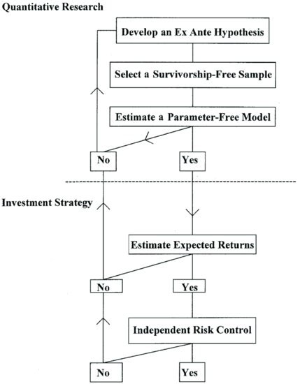
After using intuition to develop an ex ante hypothesis, the process of model selection and calibration begins in earnest. This implies selecting a sample free from biases and determining a quality-control methodology. In the production phase, an independent risk control mechanism will be essential. A key point is that the discovery process should be linear. If at any point the development process does not meet the quality standards, one should resist the temptation of adjusting parameters and go back to develop new economic intuition.
This process implies that there is plenty of economic intuition to work on. The modeler must have many ideas to develop. Ideas might range from the intuition that certain market segments have some specific behavior to the discovery that there are specific patterns of behavior with unexploited opportunities. In some cases it will be the application of ideas that are well known but have never been applied on a large scale.
A special feature of the model selection process is the level of uncertainty and noise. Models capture small amounts of information in a vast “sea of noise.” Models are always uncertain, and so is their potential longevity. The psychology of discovery plays an important role. These considerations suggest the adoption of a rigorous objective research methodology. Figure 9 illustrates the work flow for a sound process of discovery of profitable strategies. (For a further discussion, see Fabozzi, Focardi, and Ma (2005).)
Figure 9 Process of Quantitative Research and Investment Strategy
Source: Fabozzi, Focardi, and Ma (2005, p. 73)
A modeler working in financial econometrics is always confronted with the risk of finding an artifact that does not, in reality, exist. And, as we have seen, paradoxically one cannot look too hard at the data; this risks introducing biases formed by available but insufficient data sets. Even trying too many possible solutions, one risks falling into the trap of data snooping.
KEY POINTS
- Model selection in financial econometrics requires a blend of theory, creativity, and machine learning.
- The machine-learning approach starts with a set of empirical data that we want to explain. Data are explained by a family of models that include an unbounded number of parameters and are able to fit data with arbitrary precision.
- There is a trade-off between model complexity and the size of the data sample. To implement this trade-off, ensuring that models have forecasting power, the fitting of sample data is constrained to avoid fitting noise. Constraints are embodied in criteria such as the Akaike Information Criterion (AIC) or the Bayesian Information Criterion (BIC).
- Economic data are generally scarce given the complexity of their patterns. This scarcity introduces uncertainty as regards our statistical estimates. It means that the data might be compatible with many different models with the same level of statistical confidence.
- A serious mistake in model selection is to look for models that fit rare or unique patterns; such patterns are purely random and lack predictive power.
- Another mistake in model selection is data snooping, that is, fitting models to the same data that we want to explain. A sound model selection approach calls for a separation of sample data and test data: Models are fitted to sample data and tested on test data.
- Because data are scarce, techniques have been devised to make optimal use of data; perhaps the most widely used of such techniques is bootstrapping.
- Financial data are also subject to “survivorship bias,” that is, data are selected using criteria known only a posteriori, for example companies that are presently in the S&P 500. Survivorship bias induces biases in models and results in forecasting errors.
- Model risk is the risk that models are subject to forecasting errors in real data. Techniques to mitigate model risk include Bayesian techniques, averaging/shrinkage, and random coefficient models.
- A sound model selection methodology includes strong theoretical considerations, the rigorous separation of sample and testing data, and discipline to avoid data snooping.
REFERENCES
Anderson, P. W., Arrow, K. J., and Pines, D. (eds.) (1998). The Economy as an Evolving Complex System. New York: Westview Press.
Cybenko, G. (1989). Approximations by superpositions of a sigmoidal function. Mathematics of Control Signals & Systems 2: 303–314.
Davison, A. C., and Hinkley, D. V. (1997). Bootstrap Methods and Their Application. Cambridge: Cambridge University Press.
Fabozzi, F. J., Focardi, S. M., and Ma, K. C. (2005). Implementable quantitative research and investment strategies. Journal of Alternative Investment 8: 71–79.
Gleick, J. (1987). Chaos: Making a New Science. New York: Viking Penguin Books.
Glymour, C., Scheines, R., Spirtes, P., and Kelly, K. (1987). Discovering Causal Structure. Orlando, FL: Academic Press.
Gopikrishnan, P., Meyer, M., Amaral, L. A., and Stanley, H. E. (1998). Inverse cubic law for the distribution of stock price variations. The European Physical Journal B, 3: 139–140.
Plerou, V., Gopikrishnan, P., Rosenow, B., Amaral, L. A., Guhr, T., and Stanley, H. E. (2002). Random matrix approach to cross correlations in financial data. Physical Review E, 65, 066126.
Vapnik, V. N., and Chervonenkis, Y. A. (1974). Theory of Pattern Recognition (in Russian). Moscow: Nauka.
Waldrop, M. (1992). Complexity. New York: Simon & Schuster.
Yip, K. M.-K. (1989). KAM: Automatic Planning and Interpretation of Numerical Experiments Using Geometrical Methods, Ph.D. Thesis, MIT.