
The Fundamentals of Fundamental Factor Models
Fundamental analysis is the process of determining a security’s future value by analyzing a combination of macro- and microeconomic events and company-specific characteristics. Though fundamental analysis focuses on the valuation of individual companies, most institutional investors recognize that there are common factors affecting all stocks. (Common factors are shared characteristics between firms that affect their returns.) For example, macroeconomic events, like sudden changes in interest rate, inflation, or exchange rate expectations, can affect all stocks to varying degrees, depending on the stock’s characteristics.
Barr Rosenberg and Vinay Marathe (1976) developed the theory that the effects of macroeconomic events on individual securities could be captured through microeconomic characteristics—essentially common factors, such as industry membership, financial structure, or growth orientation.
Rosenberg and Marathe (1976, p. 3) discuss possible effects of a money market crisis. They say a money market crisis would:
result in possible bankruptcy for some firms, dislocation of the commercial paper market, and a dearth of new bank lending beyond existing commitments. Firms with high financial risk (shown in extreme leverage, poor coverage of fixed charges, and inadequate liquid assets) might be driven to bankruptcy. Almost all firms would suffer to some degree from higher borrowing costs and worsened economic expectations: Firms with high financial risk would be impacted most; the market portfolio, which is a weighted average of all firms, would be somewhat less exposed; and firms with abnormally low financial risk would suffer the least. Moreover, some industries such as construction would suffer greatly because of their special exposure to interest rates. Others such as liquor might be unaffected.
This early insight into the linkage between macroeconomic events and microeconomic characteristics has had a profound impact on the asset management industry ever since. In this entry, we discuss the intuition behind a fundamental factor model based on microeconomic traits, showing how it is linked to traditional fundamental analysis. When building a fundamental factor model, we look for variables that explain return, just as fundamental analysts do. We highlight the complementary role of the fundamental factor model to traditional security analysis and point out the insights these models can provide.
FUNDAMENTAL ANALYSIS AND THE BARRA FUNDAMENTAL FACTOR MODEL
Fundamental analysts use many criteria when researching companies; they may investigate a firm’s financial statements, talk to senior management, visit facilities and plants, or analyze a product pipeline. Most are seeking undervalued companies with good fundamentals or companies with strong growth potential. They typically review a range of quantitative and qualitative information to help predict future stock values. Table 1 summarizes key areas.
Table 1 Main Areas of Stock Research
| Qualitative | Quantitative |
| Business Model | Capital Structure |
| Competitive Advantage | Revenue, Expenses, and Earnings Growth |
| Management Quality | Cash Flows |
| Corporate Governance | |
| Note: Balance sheet and income statement data are readily available from 10K filings while access to company management and information about the business model and competitor landscape will vary on a case-by-case basis. | |
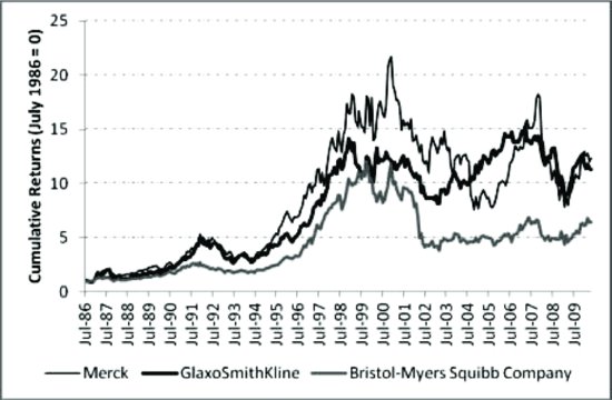
Similarly, the goal of a fundamental factor model is to identify traits that are important in forecasting security risk. These models may analyze microeconomic characteristics, such as industry membership, earnings growth, cash flow, debt-to-assets, and company specific traits. Figure 1 shows the cumulative returns to Merck, GlaxoSmithKline, and Bristol-Myers, three of the largest pharmaceutical companies in the United States. The chart illustrates the similarities in the return behavior of these stocks, primarily because they are U.S. large-cap equities within the same industry. We also see that Bristol-Myers underperformed the other two companies in recent years, indicating that other firm-specific factors also impacted its performance.
Figure 1 Industry Membership Drives Similarities between Stocks
The first task when building a fundamental factor model is to identify microeconomic traits. These include characteristics from industry membership and financial ratios to technical indicators like price momentum and recent volatility that explain return variation across a relevant security universe. The next step is to determine the impact certain events may have on individual stocks, such as the sensitivity or weight of an individual security to a change in a given fundamental factor.1 Finally, the remaining part of the returns needs to be modeled, which is the company-specific behavior of stocks.
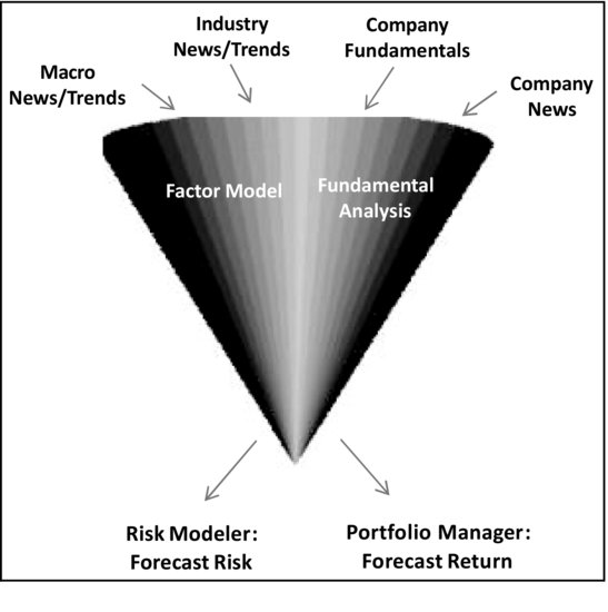
How does the model we have described compare with the way a fundamental analyst or portfolio manager analyzes stocks? The basic building blocks of analysts and factor modelers are in fact similar; both try to identify microeconomic traits that drive the risk and returns of individual securities. Figure 2 compares the two perspectives. In both views, there are clearly firm-specific traits driving risk and return. There are also sources of risk and return from a stock’s exposure, or beta, to the overall market, its industry, and certain financial and technical ratios. But the objective of the fundamental analyst is to forecast return (or future stock values), whereas the fundamental factor model forecasts the fluctuation of a security or a portfolio of securities around its expected return.
Figure 2 Overview of Stock Determinants: Fundamental Analysis versus Factor Model Analysis
Both the analyst and the factor model researcher look at similar macro- and microeconomic data and events. After all, both are seeking traits that explain the risk and returns of stocks. Table 2 shows examples used in the Barra equity models (specifically the U.S. and Japan Equity Models). Variables like profitability and debt loads are incorporated in our models through factors like Earnings Yield, Growth, and Leverage. Expectations of future revenue growth and cost savings are incorporated through variables like analyst consensus views. What about popular metrics that aren’t included? Some factors may not be good risk factors despite being good return factors. (A good return factor has persistent direction though not a lot of volatility; the ability of a company to beat earnings estimates is one of these factors). Other factors may be relevant only for a particular sector or industry. (These risk factors would only be included in industry or sector risk models.)
Table 2 Sample Fundamental Data Used in Barra Models

Note that adjustments of financial statements are incorporated in several ways. A key task for the fundamental analyst is to adjust financial statements—each analyst wants to get at the “real” number rather than what is reported in financial statements. Even under generally accepted accounting principles, management can be aggressive with basic principles, such as revenue/expense recognition; usage of unusual, infrequent, or extraordinary items; and timing issues that may lead to violations of the matching principle. In a factor model, these types of adjustments are accounted for through the inclusion of forward-looking, analyst-derived descriptors.
In addition to fundamental data, technical variables such as price momentum, beta, option-implied volatility, and so on may also be used. For instance, price momentum has been shown to significantly explain returns (see Carhart, 1997).
How are the fundamental data used in a factor model? Certain factors are found to explain stock returns over time, for example, industries and certain financial and technical ratios. If such factors explain returns across a broad universe of stocks, they are deemed important. In financial theory, these factors are “priced” across assets, for example, Fama-French value (BTM) size (small-cap) factors (Fama and French, 1992).
Once we have identified the factors, we need to link each stock to each factor. For this, we use microeconomic characteristics. We start by identifying a set of characteristics we call descriptors. For instance, if the factor is growth, a few descriptors might include earnings growth, revenue growth, and asset growth (see Table 2). These include both historical and forward-looking descriptors, such as forecast earnings growth. After we identify the important descriptors, we standardize them across a universe of stocks, typically the constituents of a broad market index.2 Table 3 illustrates how Microsoft’s exposures for the Barra U.S. factors—size, value, and yield—are calculated. We subtract the estimation universe average3 descriptor for each factor and divide it by the standard deviation of the universe of stocks.
Table 3 Calculating Exposures from Raw Data (April 1, 2010)
Table 4 Calculating Exposures When There Are Multiple Characteristics (April 1, 2010)
In some cases, factors reflect several characteristics. This occurs when multiple descriptors help explain the same factor. The Barra U.S. Growth factor, for instance, reflects five-year payouts, variability in capital structure, growth in total assets, recent large earnings changes, and forecast and historical earnings growth. Table 4 shows how we calculate Microsoft’s exposure to the Growth factor. Each descriptor is first standardized and then the descriptors are combined to form the exposure.
In addition to factors like Value, Size, Yield, and Growth, which we call style factors, a stock’s returns are also a function of its industry. Industry exposures are calculated in a different way. A company like Google, for instance, is engaged solely in Internet-related activities. It has an exposure of 100% (1.0) to the Internet industry factor in the Barra U.S. Equity Model. Its exposure to all other industry factors is zero. Some companies, like General Electric, have business activities that span multiple industries. In the U.S. model, industry exposures are based on sales, assets, and operating income in each industry.4
What does a factor exposure mean? In the same way the classic capital asset pricing model beta measures how much a stock price moves with every percentage change in the market, a factor exposure measures how much a stock price moves with every percentage change in a factor. Thus, if the value factor rises by 10%, a stock or portfolio with an exposure of 0.5 to the value factor will see a return of 5%, all else equal.5
Once we have predetermined the factor exposures for all stocks based on their underlying characteristics, we estimate the factor returns using a regression-based method.6
A stock’s return can then be described by the returns of its subcomponents: its Size exposure times the return of the Size factor plus its Value exposure times the pure return of the Value factor, and so on. This process can account for a substantial proportion of a stock’s return. The remainder of the stock’s return is deemed company specific and unique to each security. For example, the return to Microsoft over the last month can be viewed as:
![]()
where x is the exposure of Microsoft to the various factors and rFactordenotes returns to the factors.
The returns to the factors are important. They are returns to the particular style or characteristic net of all other factors. For instance, the Value factor is the return to stocks with low price to book ratio with all the industry effects and other style effects removed. Industry returns have a similar interpretation and differ from a Global Industry Classification Standard (GICS®) industry-based return. They are estimated returns that reflect the returns to that industry net of all other style characteristics. They offer insight into the pure returns to the industry.
The final building block of our fundamental factor model is the modeling of company-specific returns. Predicting specific returns and risk is a difficult task that has been approached in a number of ways. The simplest approach is to assume that specific returns and/or risk will be the same as they have been historically. Another approach is to use a structural model where the predicted specific risk of a company depends on its industry, size, and other fundamental characteristics. Both approaches—simple historical and modeled—are used in the Barra models, depending on the market. The modeled approach has the advantage of using fundamental data.
CRITICAL INSIGHTS FROM THE BARRA FUNDAMENTAL FACTOR MODEL
Fundamental analysis and fundamental factor models may begin with the same ideology but they offer different insights. Fundamental analysis ultimately focuses on in-depth company research, while factor models tie the information together at the portfolio level. The critical value of the factor model is that it shows the interaction of the firm’s microeconomic characteristics. The value of the factor model at the company level is magnified at the portfolio level as the company-specific component becomes less important. Figure 3 illustrates this principle of diversification. As names are added to the portfolio, company-specific returns are diversified away. Because the common factor (systematic) portion stays roughly the same, it becomes an increasingly larger part of the portfolio risk and return.
Figure 3 The Number of Stocks and the Impact on the Risk Composition
Note: This chart shows a stylized example of adding stocks to the portfolio where all the stocks have the same specific risk of 20%, there are two factors with risk of 10% and 5%, and correlation between them is 0.25. Factor exposures are drawn from a random distribution. Stocks are weighted equally in the portfolio.
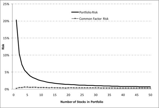
This means that at the portfolio level common factors are more important than company-specific drivers in determining a portfolio’s return and risk. Understanding and managing the common factor component becomes critical to the portfolio’s performance.
The complementary character of fundamental factor models and individual security analysis allows managers to use factor models to analyze portfolio characteristics. Next, we discuss the benefits of using fundamental factor models, including:
- Monitoring and managing portfolio exposures over time
- Understanding the contribution of factors and individual stocks to portfolio risk and tracking error relative to the relevant benchmark (risk decomposition)
- Attributing portfolio performance to factors and individual stocks to understand the return contribution of intended and accidental bets
Monitoring Portfolio Exposures
To illustrate, we use a portfolio of U.S. airline stocks. The concepts can be applied to any sector, multisector, or multicountry portfolio.
Since the middle of 2009, airline stocks have performed well. UAL (United), Delta, and Southwest saw big gains in December 2009 and February 2010. Table 5 lists the largest U.S. airline stocks as of April 30, 2010, with at least USD 1 billion market capitalization and their recent performance.
Table 5 Largest Stocks in U.S. Airline Industry and Recent Performance
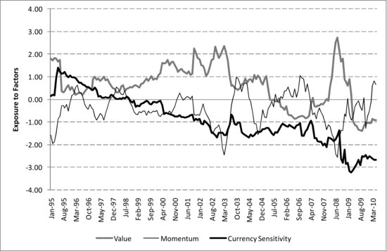
For the remainder of this section, we look at an equal-weighted portfolio of the stocks in Table 5. Figure 4 shows how the exposures of the airline portfolio to Barra factors evolved over time. The figure shows the top three exposures that changed the most in absolute terms between January 1995 and May 2010. The portfolio had an exposure to the Value factor of 1.8 in January 1995, and by May 2010 the exposure had declined to –0.9. Essentially, the portfolio went from being relatively cheap to relatively expensive during this time. Airlines have also seen a long-term decrease in exposure to currency sensitivity, most likely due to changes in oil exposure management and global air traffic patterns.
Figure 4 Airline Portfolio Exposures over Time
There can also be important differences in the distribution of the stocks’ exposures to a factor. Figure 5 shows the distribution of individual stock exposures to two of the U.S. factors—Value, which has the largest distribution, and Growth, which has among the most narrow distributions—as of May 2010. Two portfolios can have the same overall exposure to a factor but very different distributions.
Monitoring unintentional risk exposures that may not be visible on the surface can be critical. At the portfolio level, these exposures can be unintended bets that can impact overall performance. In addition, the distribution of exposures may be important. For example, a portfolio of companies with a leverage exposure of zero has a very different economic profile than a portfolio with a barbell distribution where half the companies are overleveraged and potentially vulnerable to a collapse in credit conditions.
RISK DECOMPOSITION
Factor exposures highlight how sensitive a portfolio is to different sources of risk. However, to truly understand how risky these exposures are, we can use the factor model to attribute risk fully. The combination of exposures and factor volatilities determines the riskiness of each position. For example, a portfolio can have a large exposure to a factor but if the factor isn’t particularly risky, it won’t be a major contributor to portfolio risk. Furthermore, the relationship between factors also matters. A large exposure to two factors that are highly correlated will also increase portfolio risk.
Figure 5 Monitoring the Distribution of Exposures (May 3, 2010)
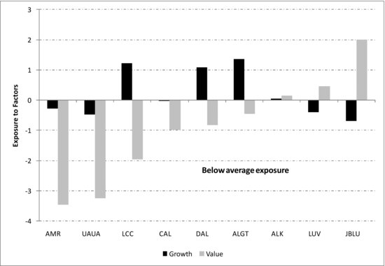
Figure 6 Sources of Risk in an Airline Portfolio, April 30, 2010, Using the Barra U.S. Equity Long-Term Model (USE3L)
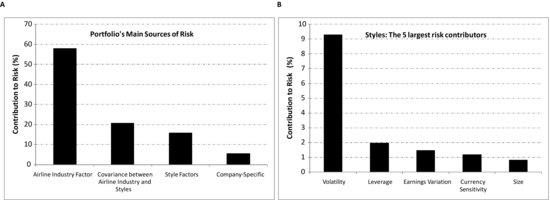
Continuing with the airline portfolio, we decompose risk as of April 30, 2010 across the four major sources (see Figure 6A). Since the stocks are within a single industry, industry risk contributes the most risk. Most importantly, we see that even with just 9 names in the portfolio, style risk far outweighs company-specific risk. The former contributes nearly three times that of the latter (16% versus 5.5%).
Table 6 Exposure to Volatility of Stocks in an Airline Portfolio, April 30, 2010, Using the Barra U.S. Long-Term Equity Model (USE3L)

Table 7 Return Attribution for Airline Portfolio and Stocks, %, March 31, 2010--April 30, 2010, Barra U.S. Equity Long-Term Model (USE3L)

Which specific style factors drive the style risk? As seen in Figure 6B, the Volatility factor is the biggest contributor by far to risk. This risk stems mostly from USAir and United’s high exposure to the factor (see Table 6).
To summarize, risk decomposition provides two critical insights. First, as we move from the stock level to the portfolio level, style and industry risk become more important, overtaking company-specific risk. Second, we see that certain styles contribute more risk than others at the stock and portfolio levels. For example, the risk of United (UAL Corp) and USAir will be heavily impacted by the Volatility factor.
Performance Attribution
The fundamental factor model also provides insight into performance attribution. Managers can use the model to analyze past performance, attributing realized portfolio return to its various sources. This can include allocations to certain countries or sectors, or allocations to certain segments—small-cap names, emerging markets, or high beta names.
Table 7 shows the decomposition of realized returns for the airline portfolio for April 2010. The first column displays the portfolio return attribution. The subsequent columns show the return attribution for each individual airline stock in isolation. The portfolio of airline stocks returned –4.3% for the month despite a positive contribution of 4.3% coming from style factors. JetBlue, for instance, was flat for the month, as its gain from style factors largely offset losses from the industry component. Similarly, Continental and UAL were helped by both strong contributions from style exposures. In contrast, positive gains from style factors were not enough to offset the company-specific losses suffered by USAir, Delta, AMR, and Allegiant. In fact, only about half the stocks realized positive company-specific returns.
Table 8 takes the last row in Table 7 and breaks it down into the individual styles in the model. The main source of positive return was the Size factor followed by the Currency Sensitivity, Leverage, and Volatility factors. In other words, airlines benefited from being smaller in cap size relative to the market (exposure of –1.7 to Size). They also benefited from the appreciation of the U.S. dollar (exposure of –2.7 to Currency Sensitivity). In addition, they were helped by being relatively levered (exposure of 2.6 to Leverage) and from having relatively higher overall and higher beta to the market (exposure of 1.7 to Volatility)
Table 8 Return Attribution for Styles Only in Percent, March 31, 2010--April 30, 2010, Barra U.S. Equity Long-Term Model (USE3L)
At the stock level, most of the airlines benefited from being relatively small. UAL and USAir benefited the most from the appreciation of the U.S. dollar. UAL, USAir, and AMR benefited the most from being relatively more levered than the other airlines. These three stocks also benefited the most from having relatively higher beta to the market and higher volatility.
Styles can contribute significantly to a manager’s performance. In our example, the U.S. Volatility factor was the main driver. Looking at individual factors and stocks, we can also see that certain factors and stocks made a significant contribution to performance due to stock-specific performance or style contribution.
In summary, portfolio performance can be strongly impacted by unintended bets. The manager may be taking major risks without adequate compensation. The factor model helps uncover these issues.
KEY POINTS
- Fundamental analysis is the process of determining a security’s future value by analyzing a combination of macro- and microeconomic events and company-specific characteristics.
- Though fundamental analysis focuses on the valuation of individual companies, most institutional investors recognize that there are common factors affecting all stocks. Common factors are shared characteristics between firms that affect their returns.
- Fundamental factor models are in fact complementary as opposed to antithetical to traditional security analysis. The basic building blocks of analysts and factor modelers are in fact similar: Both try to identify microeconomic traits that drive the risk and returns of individual securities.
- The objective of the fundamental analyst is to forecast return (or future stock values), whereas the fundamental factor model forecasts the fluctuation of a security or a portfolio of securities around its expected return. Some factors may help managers forecast return but not be good risk factors. A good return factor has persistent direction though not a lot of volatility—the ability of a company to beat earnings estimates is one of these factors. A good risk factor may be persistent or not but must be adequately volatile.
- Fundamental analysis and fundamental factor models may begin with the same ideology but they offer different insights. The most critical difference is that the factor model captures the interaction of the firm’s microeconomic characteristics at the portfolio level. This is important because as names are added to the portfolio, company-specific returns are diversified away, and the common factor (systematic) portion becomes an increasingly larger part of the portfolio risk and return.
- There are three major benefits of using fundamental factor models: (1) monitoring and managing portfolio exposures over time; (2) understanding the contribution of factors and individual stocks to portfolio risk and tracking error relative to the relevant benchmark (risk decomposition); and (3) attributing portfolio performance to factors and individual stocks to understand the return contribution of intended and accidental bets.
- Managers can use the model to analyze past performance, attributing realized portfolio return to its various sources. Portfolio performance can be strongly impacted by unintended bets. The manager may be taking major risks without adequate compensation. The factor model helps uncover these issues.
- The distribution of exposures may be important. For example, a portfolio of companies with a leverage exposure of zero has a very different economic profile than a portfolio with a barbell distribution where half the companies are overleveraged and potentially vulnerable to a collapse in credit conditions.
NOTES
1. In the Barra U.S. equity model, for example, we allow companies to be split up into five different industries, depending on their business structure.
2. All existing Barra models focus on a particular market, using an equity universe that includes all sectors and large to mid-caps with some small-caps.
3. The estimation universe average is a market-cap weighted average.
4. In effect, we build three separate valuation models. The results of each valuation model determine a set of weights, based on fundamental information. The final industry weights are a weighted average of the three weighting schemes. Further details are available in the Barra U.S. Equity Model Handbook.
5. Specifically, the effects of other factors as well as specific returns remain the same, and the risk-free rate is unchanged.
6. Details of the model construction are available in The Barra Risk Model Handbook or Barra U.S. Equity Model Handbook.
REFERENCES
Carhart, M.M. (1997). On persistence in mutual fund performance. Journal of Finance 52, 1: 57–82.
Fama, E. F., and French, K. R. (1992). The cross-section of expected stock returns. Journal of Finance 47, 2: 427–465.
Rosenberg, B., and Marathe, V. (1976). Common factors in security returns: Microeconomic determinants and macroeconomic correlates. Working paper no. 44. University of California Institute of Business and Economic Research, Research Program in Finance.