Scope and Methods of Financial Econometrics

SERGIO M. FOCARDI, PhD

Partner, The Intertek Group

FRANK J. FABOZZI, PhD, CFA, CPA

Professor of Finance, EDHEC Business School

Econometrics is the branch of economics that draws heavily on statistics for testing and analyzing economic relationships. Within econometrics, there are theoretical econometricians who analyze statistical properties of estimators of models. Several recipients of the Nobel Prize in Economic Sciences received the award as a result of their lifetime contribution to this branch of economics. To appreciate the importance of econometrics to the discipline of economics, when the first Nobel Prize in Economic Sciences was awarded in 1969, the co-recipients were two econometricians, Jan Tinbergen and Ragnar Frisch (who is credited with first using the term “econometrics” in the sense that it is known today). Further specialization within econometrics, and the subject of this entry, is financial econometrics.

As Jianqing Fan (2004) writes, financial econometrics uses statistical techniques and economic theory to address a variety of problems from finance. These include building financial models, estimation and inferences of financial models, volatility estimation, risk management, testing financial economics theory, capital asset pricing, derivative pricing, portfolio allocation, risk-adjusted returns, simulating financial systems, and hedging strategies, among others.

In this entry, we provide an overview of financial econometrics and the methods employed.

THE DATA GENERATING PROCESS

The basic principles for formulating quantitative laws in financial econometrics are the same as those that have characterized the development of quantitative science over the last four centuries. We write mathematical models, that is, relationships between different variables and/or variables in different moments and different places. The basic tenet of quantitative science is that there are relationships that do not change regardless of the moment or the place under consideration. For example, while sea waves might look like an almost random movement, in every moment and location the basic laws of hydrodynamics hold without change. Similarly, asset price behavior might appear to be random, but econometric laws should hold in every moment and for every set of assets.

There are similarities between financial eco-nometric models and models of the physical sciences, but there are also important differences. The physical sciences aim at finding immutable laws of nature; econometric models model the economy or financial markets—artifacts subject to change. For example, financial markets in the form of stock exchanges have been in operation for two centuries. During this period, they have changed significantly both in the number of stocks listed and the type of trading. And the information available on transactions has also changed. Consider that in the 1950s, we had access only to daily closing prices and this typically the day after; now we have instantaneous information on every single transaction. Because the economy and financial markets are artifacts subject to change, econometric models are not unique representations valid throughout time; they must adapt to the changing environment.

While basic physical laws are expressed as differential equations, financial econometrics uses both continuous-time and discrete-time models. For example, continuous-time models are used in modeling derivatives where both the underlying and the derivative price are represented by stochastic (i.e., random) differential equations. In order to solve stochastic differential equations with computerized numerical methods, derivatives are replaced with finite differences. (Note that the stochastic nature of differential equations introduces fundamental mathematical complications. The definition of stochastic differential equations is a delicate mathematical process invented, independently, by the mathematicians Ito and Stratonovich. In the Ito-Stratonovich definition, the path of a stochastic differential equation is not the solution of a corresponding differential equation. However, the numerical solution procedure yields a discrete model that holds pathwise. See Focardi and Fabozzi [2004].) This process of discretization of time yields discrete time models. However, discrete time models used in financial econometrics are not necessarily the result of a process of discretization of continuous time models.

Let’s focus on models in discrete time, the bread-and-butter of econometric models used in asset management. There are two types of discrete-time models: static and dynamic. Static models involve different variables at the same time. The well-known capital asset pricing model (CAPM), for example, is a static model. Dynamic models involve one or more variables at two or more moments. (This is true in discrete time. In continuous time, a dynamic model might involve variables and their derivatives at the same time.) Momentum models, for example, are dynamic models.

In a dynamic model, the mathematical relationship between variables at different times is called the data generating process (DGP). This terminology reflects the fact that, if we know the DGP of a process, we can simulate the process recursively, starting from initial conditions. Consider the time series of a stock price pt, that is, the series formed with the prices of that stock taken at fixed points in time, say daily. Let’s now write a simple econometric model of the prices of a stock as follows:

(1)

This model tells us that if we consider any time t+1, the price of that stock at time t+1 is equal to a constant plus the price in the previous moment t multiplied by ρ plus a zero-mean random disturbance independent from the past, which always has the same statistical characteristics. If we want to apply this model to real-world price processes, the constants μ and ρ must be estimated. The parameter μ determines the trend and ρ defines the dependence between the prices. Typically ρ is less than but close to 1. A random disturbance of the type shown in the above equation is called a white noise.

If we know the initial price p0 at time t = 0, using a computer program to generate random numbers, we can simulate a path of the price process with the following recursive equations:

That is, we can compute the price at time t = 1 from the initial price p0 and a computer-generated random number ε1 and then use this new price to compute the price at time t = 2, and so on. The εi are independent and identically distributed random variables with zero mean. Typical choices for the distribution of ε are normal distribution, t-distribution, and stable non-Gaussian distribution. The distribution parameters are estimated from the sample.

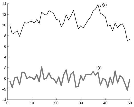
Figure 1 DGP and Noise Terms

It is clear that if we have a DGP we can generate any path. An econometric model that involves two or more different times can be regarded as a DGP. However, there is a more general way of looking at econometric models that encompasses both static and dynamic models. That is, we can look at econometric models from a perspective other than that of the recursive generation of stochastic paths. In fact, we can rewrite our previous model as follows:

(2)

This formulation shows that, if we consider any two consecutive instants of time, there is a combination of prices that behave as random noise. More in general, an econometric model can be regarded as a mathematical device that reconstructs a noise sequence from empirical data.

This concept is visualized in Figure 1, which shows a time series of numbers pt generated by a computer program according to the rule given by (2) with ρ = 0.9 and μ = 1 and the corresponding time series εt. If we choose any pair of consecutive points in time, say (t+1,t), the difference pt+1 – μ – ρ pt is always equal to the series εt+1. For example, consider the points p13 = 10.2918, p14 = 12.4065. The difference p14 – 0.9p13 – 1 = 2.1439 has the same value as ε14. If we move to a different pair we obtain the same result, that is, if we compute pt+1 – 1 – 0.9pt, the result will always be the noise sequence εt+1.

To help intuition, imagine that our model is a test instrument: Probing our time series with our test instrument, we always obtain the same reading. Actually, what we obtain is not a constant reading but a random reading with mean zero and fixed statistical characteristics. The objective of financial econometrics is to find possibly simple expressions of different financial variables such as prices, returns, or financial ratios in different moments that always yield, as a result, a zero-mean random disturbance.

Static models (i.e., models that involve only one instant) are used to express relationships between different variables at any given time. Static models are used, for example, to determine exposure to different risk factors. However, because they involve only one instant, static models cannot be used to make forecasts; forecasting requires models that link variables in two or more instants in time.

FINANCIAL ECONOMETRICS AT WORK

Applying financial econometrics involves three key steps: (1) model selection, (2) model estimation, and (3) model testing.

In the first step, model selection, the modeler chooses (or might write ex novo) a family of models with given statistical properties. This entails the mathematical analysis of the model properties as well as economic theory to justify the model choice. It is in this step that the modeler decides to use, for example, regression on financial ratios or other variables to model returns.

In general, models include a number of free parameters that have to be estimated from sample data, the second step in applying financial econometrics. Suppose that we have decided to model returns with a regression model. This requires the estimation of the regression coefficients, performed using historical data. Estimation provides the link between reality and models. As econometric models are probabilistic models, any model can in principle describe our empirical data. We choose a family of models in the model selection phase and then determine the optimal model in the estimation phase.

As mentioned, model selection and estimation are performed on historical data. As models are adapted (or fitted) to historical data there is always the risk that the fitting process captures ephemeral features of the data. Thus there is the need to test the models on data different from the data on which the models were estimated. This is the third step in applying financial econometrics, model testing. We assess the performance of models on fresh data.

We can take a different approach to model selection and estimation, namely statistical learning. Statistical learning combines the two steps—model selection and model estimation—insofar as it makes use of a class of universal models that can fit any data. Neural networks are an example of universal models. The critical step in the statistical learning approach is estimation. This calls for methods to restrict model complexity (i.e., the number of parameters used in a model).

Within this basic scheme for applying financial econometrics, we can now identify a number of modeling issues, such as:

• How do we apply statistics given that there is only one realization of financial series?
• Given a sample of historical data, how do we choose between linear and nonlinear models, or the different distributional assumptions or different levels of model complexity?
• Can we exploit more data using, for example, high-frequency data?
• How can we make our models more robust, reducing model risk?
• How do we measure not only model performance but also the ability to realize profits?

Implications of Empirical Series with Only One Realization

As mentioned, econometric models are probabilistic models: Variables are random variables characterized by a probability distribution. Generally speaking, probability concepts cannot be applied to single “individuals” (at least, not if we use a frequentist concept of probability). Probabilistic models describe “populations” formed by many individuals. However, empirical financial time series have only one realization. For example, there is only one historical series of prices for each stock—and we have only one price at each instant of time. This makes problematic the application of probability concepts. How, for example, can we meaningfully discuss the distribution of prices at a specific time given that there is only one price observation? Applying probability concepts to perform estimation and testing would require populations made up of multiple time series and samples made up of different time series that can be considered a random draw from some distribution.

As each financial time series is unique, the solution is to look at the single elements of the time series as the individuals of our population. For example, because there is only one realization of each stock’s price time series, we have to look at the price of each stock at different moments. However, the price of a stock (or of any other asset) at different moments is not a random independent sample. For example, it makes little sense to consider the distribution of the prices of a single stock in different moments because the level of prices typically changes over time. Our initial time series of financial quantities must be transformed; that is, a unique time series must be transformed into populations of individuals to which statistical methods can be applied. This holds not only for prices but for any other financial variable.

Econometrics includes transformations of the above type as well as tests to verify that the transformation has obtained the desired result. The DGP is the most important of these transformations. Recall that we can interpret a DGP as a method for transforming a time series into a sequence of noise terms. The DGP, as we have seen, constructs a sequence of random disturbances starting from the original series; it allows one to go backwards and infer the statistical properties of the series from the noise terms and the DGP. However, these properties cannot be tested independently.

The DGP is not the only transformation that allows statistical estimates. Differencing time series, for example, is a process that may transform nonstationary time series into stationary time series. A stationary time series has a constant mean that, under specific assumptions, can be estimated as an empirical average.

Determining the Model

As we have seen, econometric models are mathematical relationships between different variables at different times. An important question is whether these relationships are linear or nonlinear. Consider that every econometric model is an approximation. Thus the question is: Which approximation—linear or nonlinear—is better?

To answer this, it is generally necessary to consider jointly the linearity of models, the distributional assumptions, and the number of time lags to introduce. The simplest models are linear models with a small number of lags under the assumption that variables are normal variables. A widely used example of normal linear models are regression models where returns are linearly regressed on lagged factors under the assumption that noise terms are normally distributed. A model of this type can be written as:

(3)

where rt are the returns at time t and ft are factors, that is, economic or financial variables. Given the linearity of the model, if factors and noise are jointly normally distributed, returns are also normally distributed.

However, the distribution of returns, at least at some time horizons, is not normal. If we postulate a nonlinear relationship between factors and returns, normally distributed factors yield a non-normal return distribution. However, we can maintain the linearity of the regression relationship but assume a non-normal distribution of noise terms and factors. Thus nonlinear models transform normally distributed noise into non-normal variables but it is not true that non-normal distributions of variables implies nonlinear models.

If we add lags (i.e., a time space backward), the above model becomes sensitive to the shape of the factor paths. For example, a regression model with two lags will behave differently if the factor is going up or down. Adding lags makes models more flexible but more brittle. In general, the optimal number of lags is dictated not only by the complexity of the patterns that we want to model but also by the number of points in our sample. If sample data are abundant, we can estimate a rich model.

Typically there is a trade-off between model flexibility and the size of the data sample. By adding time lags and nonlinearities, we make our models more flexible, but the demands in terms of estimation data are greater. An optimal compromise has to be made between the flexibility given by nonlinear models and/or multiple lags and the limitations due to the size of the data sample.

TIME HORIZON OF MODELS

There are trade-offs between model flexibility and precision that depend on the size of sample data. To expand our sample data, we would like to use data with small time spacing in order to multiply the number of available samples. High-frequency data or HFD (i.e., data on individual transactions) have the highest possible frequency (i.e., each individual transaction) and are irregularly spaced. To give an idea of the ratio in terms of numbers, consider that there are approximately 2,100 ticks per day for the median stock in the Russell 3000 (see Falkenberry, 2002). Thus the size of the HDF data set of one day for a typical stock in the Russell 3000 is 2,100 times larger than the size of closing data for the same day!

In order to exploit all available data, we would like to adopt models that work over time intervals of the order of minutes and, from these models, compute the behavior of financial quantities over longer periods. Given the number of available sample data at high frequency, we could write much more precise laws than those established using longer time intervals. Note that the need to compute solutions over forecasting horizons much longer than the time spacing is a general problem that applies at any time interval. For example, in asset allocation we need to understand the behavior of financial quantities over long time horizons. The question we need to ask is if models estimated using daily intervals can correctly capture the process dynamics over longer periods, such as years.

It is not necessarily true that models estimated on short time intervals, say minutes, offer better forecasts at longer time horizons than models estimated on longer time intervals, say days. This is because financial variables might have a complex short-term dynamics superimposed on a long-term dynamics. It might be that using high-frequency data, one captures the short-term dynamics without any improvement in the estimation of the long-term dynamics. That is, with high-frequency data it might be that models get more complex (and thus more data-hungry) because they describe short-term behavior superimposed on long-term behavior. This possibility must be resolved for each class of models.

Another question is if it is possible to use the same model at different time horizons. To do so is to imply that the behavior of financial quantities is similar at different time horizons. This conjecture was first made by Benoit Mandelbrot (1963), who observed that long series of cotton prices were very similar at different time aggregations.

Model Risk and Model Robustness

Not only are econometric models probabilistic models, as we have already noted; they are only approximate models. That is, the probability distributions themselves are only approximate and uncertain. The theory of model risk and model robustness assumes that all parameters of a model are subject to uncertainty and attempts to determine the consequence of model uncertainty and strategies for mitigating errors.

The growing use of models in finance has heightened the attention to model risk and model-risk mitigation techniques. Asset management firms are beginning to address the need to implement methodologies that allow both robust estimation and robust optimization in the portfolio management process.

Performance Measurement of Models

It is not always easy to understand ex ante just how well (or how poorly) a forecasting model will perform. Because performance evaluations made on training data are not reliable, the evaluation of model performance requires separate data sets for training and for testing. Models are estimated on training data and tested on the test data. Poor performance might be due to model misspecification, that is, models might not reflect the true DGP of the data (assuming one exists), or there might simply be no DGP.

Various measures of model performance have been proposed. For example, one can compute the correlation coefficient between the forecasted variables and their actual realizations. Each performance measure is a single number and therefore conveys only one aspect of the forecasting performance. Often it is crucial to understand if errors can become individually very large or if they might be correlated. Note that a simple measure of model performance does not ensure the profitability of strategies. This can be due to a number of reasons, including, for example, the risk inherent in apparently profitable forecasts, market impact, and transaction costs.

APPLICATIONS

There has been a greater use of econometric models in investment management since the turn of the century. Application areas include:

• Portfolio construction and optimization
• Risk management
• Asset and liability management

Each type of application requires different modeling approaches.

Portfolio Construction and Optimization

Portfolio construction and optimization require models to forecast returns: There is no way to escape the need to predict future returns. Passive strategies apparently eschew the need to forecast future returns of individual stocks by investing in broad indexes. They effectively shift the need to forecast to a higher level of analysis and to longer time horizons.

Until recently, the mainstream view was that financial econometric models could perform dynamic forecasts of volatility but not of expected returns. However, volatility forecasts are rarely used in portfolio management. With the exception of some proprietary applications, the most sophisticated models used in portfolio construction until recently were factor models where forecasts are not dynamic but consist in estimating a drift (i.e., a constant trend) plus a variance-covariance matrix.

Since the late 1990s, the possibility of making dynamic forecasts of both volatility and expected returns has gained broad acceptance. During the same period, it became more widely recognized that returns are not normally distributed, evidence that had been reported by Mandelbrot (1963). Higher moments of distributions are therefore important in portfolio management and therefore require representation and estimation of nonnormal distributions.

As observed above, the ability to correctly forecast expected returns does not imply, per se, that there are profit opportunities. In fact, we have to take into consideration the interplay between expected returns, higher moments, and transaction costs. As dynamic forecasts typically involve higher portfolio turnover, transaction costs might wipe out profits. As a general comment, portfolio management based on dynamic forecasts calls for a more sophisticated framework for optimization and risk management with respect to portfolio management based on static forecasts.

Regression models appear to form the core of the modeling efforts to predict future returns at many asset management firms. Regression models regress returns on a number of predictors. Stated otherwise, future returns are a function of the value of present and past predictors. Predictors include financial ratios such as earning-to-price ratio or book-to-price ratio and other fundamental quantities; predictors might also include behavioral variables such as market sentiment. A typical formula of a regressive model is the following:

(4)

where

is the return at time t+1 of the i-th asset, and the fj,t are factors observed at time t. While regressions are generally linear, nonlinear models are also used.

In general, the forecasting horizon in asset management varies from a few days for actively managed or hedge funds to several weeks for more traditionally managed funds. Dynamic models typically have a short forecasting horizon as they capture short-term dynamics. This contrasts with static models, such as the widely used multifactor models, which tend to capture long-term trends and ignore short-term dynamics.

The evolution of forecasting models over the last two decades has also changed the way forecasts are used. A basic utilization of forecasts is in stock picking/ranking systems, which have been widely implemented at asset management firms. The portfolio manager builds his or her portfolio combining the model ranking with the manager’s personal views and within the constraints established by the firm. A drawback in using such an approach is the difficulty in properly considering the structure of correlations and the role of higher moments.

Alternatively, forecasts can be fed to an optimizer that automatically computes the portfolio weights. But because an optimizer implements an optimal trade-off between returns and some measure of risk, the forecasting model must produce not only returns forecasts but also measures of risk. If risk is measured by portfolio variance or standard deviation, the forecasting model must be able to provide an estimated variance-covariance matrix.

Estimating the variance-covariance matrix is the most delicate of the estimation tasks. Here is why. The number of entries of a variance-covariance matrix grows with the square of the number of stocks. As a consequence, the number of entries in a variance-covariance matrix rapidly becomes very large. For example, the variance-covariance matrix of the stocks in the S&P 500 is a symmetric matrix that includes some 125,000 entries. If our universe were the Russell 5000, the variance-covariance matrix would include more than 12 million entries. The problem with estimating matrices of this size is that estimates are very noisy because the number of sample data is close to the number of parameters to estimate. For example, if we use three years of data for estimation, we have, on average, less than three data points per estimated entry in the case of the S&P 500; in the case of the Russell 5000, the number of data points would be one fourth of the number of entries to estimate! Robust estimation methods are called for.

Note that if we use forecasting models we typically have (1) an equilibrium variance-covariance matrix that represents the covariances of the long-run relationships between variables, plus (2) a short-term, time-dependent, variance-covariance matrix. If returns are not normally distributed, optimizers might require the matrix of higher moments.

A third utilization of forecasting models and optimizers is to construct model portfolios. In other words, the output of the optimizer is used to construct not an actual but a model portfolio. This model portfolio is used as input by portfolio managers.

Risk Management

Risk management has different meanings in different contexts. In particular, when optimization is used, risk management is intrinsic to the optimization process, itself a risk-return trade-off optimization. In this case, risk management is an integral part of the portfolio construction process.

However, in most cases, the process of constructing portfolios is entrusted to human portfolio managers who might use various inputs including, as noted above, ranking systems or model portfolios. In these cases, portfolios might not be optimal from the point of view of risk management and it is therefore necessary to ensure independent risk oversight. This oversight might take various forms. One form is similar to the type of risk oversight adopted by banks. The objective is to assess potential deviations from expectations. In order to perform this task, the risk manager receives as input the composition of portfolios and makes return projections using static forecasting models.

Another form of risk oversight, perhaps the most diffused in portfolio management, assesses portfolio exposures to specific risk factors. As portfolio management is often performed relative to a benchmark and risk is defined as underperformance relative to the benchmark, it is important to understand the sensitivity of portfolios to different risk factors. This type of risk oversight does not entail the forecasting of returns. The risk manager uses various statistical techniques to estimate how portfolios move in function of different risk factors. In most cases, linear regressions are used. A typical model will have the following form:

(5)

where

is the return observed at time t of the i-th asset, and the fj,t are factors observed at time t. Note that this model is fundamentally different from a regressive model with time lags as given by (4).

Asset-Liability Management

Asset-liability management (ALM) is typical of those asset management applications that require the optimization of portfolio returns at some fixed time horizon plus a stream of consumption throughout the entire life of the portfolio. ALM is important for managing portfolios of institutional investors such as pension funds or foundations. It is also important for wealth management, where the objective is to cover the investor’s financial needs over an extended period.

ALM requires forecasting models able to capture the asset behavior at short-, medium-, and long-term time horizons. Models of the long-term behavior of assets exist but are clearly difficult to test. Important questions related to these long-term forecasting models include:

• Do asset prices periodically revert to one or many common trends in the long run?
• Can we assume that the common trends (if they exist) are deterministic trends such as exponentials or are common trends stochastic (i.e., random) processes?
• Can we recognize regime shifts over long periods of time?

KEY POINTS

• Financial econometrics employs the same basic principles for formulating quantitative laws that characterized the development of quantitative science.
• Although there are similarities between financial econometric models and models of the physical sciences, important differences exist. For example, physical sciences seek immutable laws of nature, while econometric models model the economy or financial markets, which are artifacts subject to change.
• Econometric models are mathematical relationships between different variables at different times, and every econometric model is an approximation.
• Both continuous-time and discrete-time models are used in financial econometrics.
• Static models express relationships between different variables at any given time. Because they involve only one instant in time, static models cannot be used to make forecasts since to do so models that link variables in two or more instants in time are required.
• Dynamic models involve one or more variables at two or more points in time; the data generating process in dynamic models is the mathematical relationship between variables at different times.
• Applying financial econometrics involves three key steps: (1) model selection, (2) model estimation, and (3) model testing.
• In model selection, the modeler selects the model based on an assessment of a model’s properties and its fit to economic theory.
• Estimation provides the link between reality and models. In model estimation, the modeler applies financial econometric techniques to estimate the model’s free parameters from sample data.
• The evaluation of model performance requires separate data sets for training and for testing because performance evaluations made on training data are not reliable.
• In investment management there has been increased use of econometric models in portfolio construction and optimization, risk management, and asset and liability management. A different modeling approach is needed for each type of application.

REFERENCES

Falkenberry, T. N. (2002). High frequency data filtering. Tick Data Inc.

Fan, J. (2004). An introduction to financial econometrics. Unpublished paper, Department of Operations Research and Financial Engineering, Princeton University.

Focardi, S. M., and Fabozzi, F. J. (2004). The Mathematics of Financial Modeling and Investment Management. Hoboken, NJ: John Wiley & Sons.

Mandelbrot, B. (1963). The variation of certain speculative prices. Journal of Business 36: 394–419.