
Principal Components Analysis and Factor Analysis
Principal component analysis (PCA) and factor analysis are statistical tools that allow a modeler to (1) reduce the number of variables in a model (i.e., to reduce the dimensionality), and (2) identify if there is structure in the relationships between variables (i.e., to classify variables). In this entry, we explain PCA and factor analysis. We illustrate and compare both techniques using a sample of stocks. Because of its use in the estimation of factor models, we begin with a brief discussion of factor models.
FACTOR MODELS
Factor models are statistical models that try to explain complex phenomena through a small number of basic causes or factors. Factor models serve two main purposes: (1) They reduce the dimensionality of models to make estimation possible; and/or (2) they find the true causes that drive data. Factor models were introduced by Charles Spearman (1904), a leading psychologist who developed many concepts of modern psychometrics.
Spearman was particularly interested in understanding how to measure human intellectual abilities. In his endeavor to do so, he developed the first factor model, known as the Spearman model, a model that explains intellectual abilities through one common factor, the famous “general intelligence” g factor, plus another factor s, which is specific to each distinct ability. Spearman was persuaded that the factor g had an overwhelming importance. That is, he thought that any mental ability can be explained quantitatively through a common intelligence factor. According to this theory, outstanding achievements of, say, a painter, a novelist, and a scientist can all be ascribed to a common general intelligence factor plus a small contribution from specific factors.
Some 30 years later, Louis Leon Thurstone (1938) developed the first true multifactor model of intelligence. Thurstone was among the first to propose and demonstrate that there are numerous ways in which a person can be intelligent. Thurstone’s multiple-factors theory identified seven primary mental abilities.
One might question whether factors are only statistical artifacts or if they actually correspond to any reality. In the modern operational interpretation of science, a classification or a factor is “real” if we can make useful predictions using that classification. For example, if the Spearman theory is correct, we can predict that a highly intelligent person can obtain outstanding results in any field. Thus, a novelist could have obtained outstanding results in science. However, if many distinct mental factors are needed, people might be able to achieve great results in some field but be unable to excel in others.
In the early applications of factor models to psychometrics, the statistical model was essentially a conditional multivariate distribution. The raw data were large samples of psychometric tests. The objective was to explain these tests as probability distributions conditional on the value of one or more factors. In this way, one can make predictions of, for example, the future success of young individuals in different activities.
In finance, factor models are typically applied to time series. The objective is to explain the behavior of a large number of stochastic processes, typically price, returns, or rate processes, in terms of a small number of factors. These factors are themselves stochastic processes. In order to simplify both modeling and estimation, most factor models employed in financial econometrics are static models. This means that time series are assumed to be sequences of temporally independent and identically distributed (IID) random variables so that the series can be thought of as independent samples extracted from one common distribution.
In financial econometrics, factor models are needed not only to explain data but to make estimation feasible. Given the large number of stocks presently available—in excess of 15,000—the estimation of correlations cannot be performed without simplifications. Widely used ensembles such as the S&P 500 or the MSCI Europe include hundreds of stocks and therefore hundreds of thousands of individual correlations. Available samples are insufficient to estimate this large number of correlations. Hence factor models are able to explain all pairwise correlations in terms of a much smaller number of correlations between factors.
Linear Factor Models Equations
Linear factor models are regression models of the following type:
![]()
where
Xi = a set of N random variables
fj = a set of K common factors
εi = the noise terms associated with each variable Xi
The βij’s are called the factor loadings or factor sensitivities; they express the influence of the j-th factor on the i-th variable.
In this formulation, factor models are essentially static models, where the variables and the factors are random variables without any explicit dependence on time. It is possible to add a dynamic to both the variables and the factors, but that is beyond the scope of our basic introduction in this entry.
As mentioned above, one of the key objectives of factor models is to reduce the dimensionality of the covariance matrix so that the covariances between the variables Xi are determined only by the covariances between factors. Suppose that the noise terms are mutually uncorrelated, so that
![]()
and that the noise terms are uncorrelated with the factors, that is, E(εifj) = 0, ∀i,j. Suppose also that both factors and noise terms have a zero mean, so that E(Xi) = αi. Factor models that respect the above constraints are called strict factor models.
Let’s compute the covariances of a strict factor model:
From this expression we can see that the variances and covariances between the variables Xi depend only on the covariances between the factors and the variances of the noise term.
We can express the above compactly in matrix form. Let’s write a factor model in matrix form as follows:
![]()
where
X = (X1, … , XN)′ = the N-vector of variables
α = (α1, … , αN)′ = the N-vector of means
ε = (ε1, … , εN)′ = the N-vector of idiosyncratic noise terms
f = (f1, … , fK)′ = the K-vector of factors
Let’s define the following:
where
Σ = the N × N variance-covariance matrix of the variables X
Ω = the K × K variance-covariance matrix of the factors
Ψ = N × N variance-covariance matrix of the error terms ε
If we assume that our model is a strict factor model, the matrix ![]() will be a diagonal matrix with the noise variances on the diagonal, that is,
will be a diagonal matrix with the noise variances on the diagonal, that is,
Under the above assumptions, we can express the variance-covariance matrix of the variables in the following way:
![]()
In practice, the assumption of a strict factor model might be too restrictive. In applied work, factor models will often be approximate factor models. (See, for example, Bai, 2003.) Approximate factor models allow idiosyncratic terms to be weakly correlated among themselves and with the factors.
As many different factor models have been proposed for explaining stock returns, an important question is whether a factor model is fully determined by the observed time series. In a strict factor model, factors are determined up to a nonsingular linear transformation. In fact, the above matrix notation makes it clear that the factors, which are hidden, nonobservable variables, are not fully determined by the above factor model. That is, an estimation procedure cannot univocally determine the hidden factors and the factor loadings from the observable variables X. In fact, suppose that we multiply the factors by any nonsingular matrix R. We obtain other factors
![]()
with a covariance matrix
![]()
and we can write a new factor model:
![]()
In order to solve this indeterminacy, we can always choose the matrix R so that the factors g are a set of orthonormal variables, that is, uncorrelated variables (the orthogonality condition) with unit variance (the normality condition). In order to make the model uniquely identifiable, we can stipulate that factors must be a set of orthonormal variables and that, in addition, the matrix of factor loadings is diagonal. Under this additional assumption, a strict factor model is called a normal factor model. Note explicitly that under this assumption, factors are simply a set of standardized independent variables. The model is still undetermined under rotation, that is multiplication by any nonsingular matrix such that RR′ = I.
In summary, a set of variables has a normal factor representation if it is represented by the following factor model:
![]()
where factors are orthonormal variables and noise terms are such that the covariance matrix can be represented as follows:
![]()
where β is the diagonal matrix of factor loadings and ![]() is a diagonal matrix.
is a diagonal matrix.
How can we explain the variety of factor models proposed given that a strict factor model could be uniquely identified up to a factor linear transformation? As mentioned, the assumptions underlying strict factor models are often too restrictive and approximate factor models have to be adopted. Approximate factor models are uniquely identifiable only in the limit of an infinite number of series. The level of approximation is implicit in practical models of returns.
Types of Factors and Their Estimation
In financial econometrics, the factors used in factor models can belong to three different categories: macroeconomic factors, fundamental factors, and statistical factors. The first two are factor models that deal with known factors and will not be discussed here.
Note that factors defined through statistical analysis are linear combinations of the variables. That is, if the variables are asset returns, factors are portfolios of assets. They are hidden variables insofar as one does not know the weights of the linear combinations. However, once the estimation process is completed, statistical factors are always linear combinations of variables. If data have a strict factor structure, we can always construct linear combinations of the series (e.g., portfolios of returns) that are perfectly correlated with a set of factors. Often they can be given important economic interpretations. In the following sections we describe the theory and estimation methods of principal components analysis and factor analysis.
PRINCIPAL COMPONENTS ANALYSIS
Principal components analysis (PCA) was introduced by Harold Hotelling (1933). Hotelling proposed PCA as a way to determine factors with statistical learning techniques when factors are not exogenously given. Given a variance-covariance matrix, one can determine factors using the technique of PCA.
PCA implements a dimensionality reduction of a set of observations. The concept of PCA is the following. Consider a set of n stationary time series Xi, for example the 500 series of returns of the S&P 500. Consider next a linear combination of these series, that is, a portfolio of securities. Each portfolio P is identified by an n-vector of weights ωP and is characterized by a variance σp2. In general, the variance σp2 depends on the portfolio’s weights ωP. Lastly, consider a normalized portfolio, which has the largest possible variance. In this context, a normalized portfolio is a portfolio such that the squares of the weights sum to one.
If we assume that returns are IID sequences, jointly normally distributed with variance-covariance matrix σ, a lengthy direct calculation demonstrates that each portfolio’s return will be normally distributed with variance
![]()
The normalized portfolio of maximum variance can therefore be determined in the following way:
![]()
subject to the normalization condition
![]()
where the product is a scalar product. It can be demonstrated that the solution of this problem is the eigenvector ω1 corresponding to the largest eigenvalue λ1 of the variance-covariance matrix σ. As σ is a variance-covariance matrix, the eigenvalues are all real.
Consider next the set of all normalized portfolios orthogonal to ω1, that is, portfolios completely uncorrelated with ω1. These portfolios are identified by the following relationship:
![]()
We can repeat the previous reasoning. Among this set, the portfolio of maximum variance is given by the eigenvector ω2 corresponding to the second largest eigenvalue λ2 of the variance-covariance matrix σ. If there are n distinct eigenvalues, we can repeat this process n times. In this way, we determine the n portfolios Pi of maximum variance. The weights of these portfolios are the orthonormal eigenvectors of the variance-covariance matrix σ. Note that each portfolio is a time series that is a linear combination of the original time series Xi. The coefficients are the portfolios’ weights.
These portfolios of maximum variance are all mutually uncorrelated. It can be demonstrated that we can recover all the original return time series as linear combinations of these portfolios:
![]()
Thus far we have succeeded in replacing the original n correlated time series Xj with n uncorrelated time series Pi with the additional insight that each Xj is a linear combination of the Pi. Suppose now that only p of the portfolios Pi have a significant variance, while the remaining n − p have very small variances. We can then implement a dimensionality reduction by choosing only those portfolios whose variance is significantly different from zero. Let’s call these portfolios factors F.
It is clear that we can approximately represent each series Xi as a linear combination of the factors plus a small uncorrelated noise. In fact we can write
![]()
where the last term is a noise term. Therefore to implement PCA one computes the eigenvalues and the eigenvectors of the variance-covariance matrix and chooses the eigenvalues significantly different from zero. The corresponding eigenvectors are the weights of portfolios that form the factors. Criteria of choice are somewhat arbitrary.
Suppose, however, that there is a strict factor structure, which means that returns follow a strict factor model as defined earlier in this entry:
![]()
The matrix β can be obtained diagonalizing the variance-covariance matrix. In general, the structure of factors will not be strict and one will try to find an approximation by choosing only the largest eigenvalues.
Note that PCA works either on the variance-covariance matrix or on the correlation matrix. The technique is the same but results are generally different. PCA applied to the variance-covariance matrix is sensitive to the units of measurement, which determine variances and covariances. This observation does not apply to returns, which are dimensionless quantities. However, if PCA is applied to prices and not to returns, the currency in which prices are expressed matters; one obtains different results in different currencies. In these cases, it might be preferable to work with the correlation matrix.
We have described PCA in the case of time series, which is the relevant case in econometrics. However, PCA is a generalized dimensionality reduction technique applicable to any set of multidimensional observations. It admits a simple geometrical interpretation, which can be easily visualized in the three-dimensional case. Suppose a cloud of points in the three-dimensional Euclidean space is given. PCA finds the planes that cut the cloud of points in such a way as to obtain the maximum variance.
Illustration of Principal Components Analysis
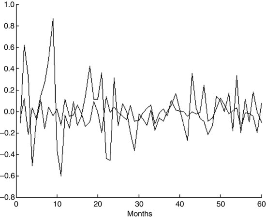
Let’s now show how PCA is performed. To do so, we used monthly observations for the following 10 stocks: Campbell Soup, General Dynamics, Sun Microsystems, Hilton, Martin Marietta, Coca-Cola, Northrop Grumman, Mercury Interactive, Amazon.com, and United Technologies for the period from December 2000 to November 2005. Figure 1 shows the graphics of the 10 return processes.
As explained earlier, performing PCA is equivalent to determining the eigenvalues and eigenvectors of the covariance matrix or of the correlation matrix. The two matrices yield different results. We perform both exercises, estimating the principal components using separately the covariance and the correlation matrices of the return processes. We estimate the covariance with the empirical covariance matrix. Recall that the empirical covariance σij between variables (Xi,Xj) is defined as follows:
Table 1 shows the covariance matrix.
Figure 1 Graphics of the 10 Stock Return Processes
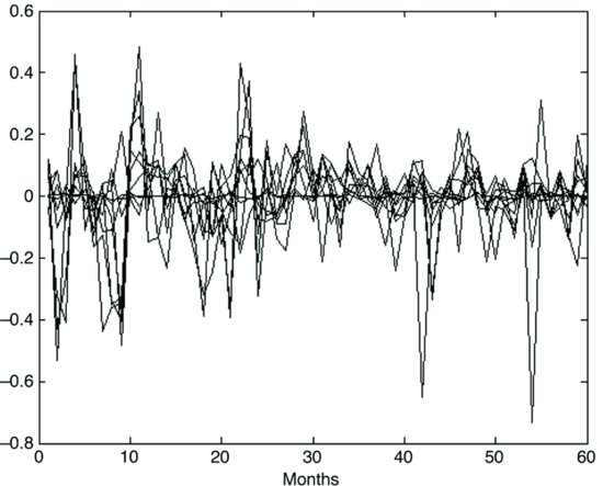
Table 1 The Covariance Matrix of 10 Stock Returns
Normalizing the covariance matrix with the standard deviations, we obtain the correlation matrix. Table 2 shows the correlation matrix. Note that the diagonal elements of the correlation matrix are all equal to one. In addition, a number of entries in the covariance matrix are close to zero. Normalization by the product of standard deviations makes the same elements larger.
Table 2 The Correlation Matrix of the Same 10 Return Processes

Let’s now proceed to perform PCA using the covariance matrix. We have to compute the eigenvalues and the eigenvectors of the covariance matrix. Table 3 shows the eigenvectors (panel A) and the eigenvalues (panel B) of the covariance matrix.
Table 3 Eigenvectors and Eigenvalues of the Covariance Matrix

Each column of panel A of Table 3 represents an eigenvector. The corresponding eigenvalue is shown in panel B. Eigenvalues are listed in descending order; the corresponding eigenvectors go from left to right in the matrix of eigenvectors. Thus the leftmost eigenvector corresponds to the largest eigenvalue. Eigenvectors are not uniquely determined. In fact, multiplying any eigenvector for a real constant yields another eigenvector. The eigenvectors in Table 3 are normalized in the sense that the sum of the squares of each component is equal to 1. It can be easily checked that the sum of the squares of the elements in each column is equal to 1. This still leaves an indeterminacy, as we can change the sign of the eigenvector without affecting this normalization.
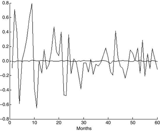
As explained earlier, if we form portfolios whose weights are the eigenvectors, we can form 10 portfolios that are orthogonal (i.e., uncorrelated). These orthogonal portfolios are called principal components. The variance of each principal component will be equal to the corresponding eigenvector. Thus the first principal component (i.e., the portfolio corresponding to the first eigenvalue), will have the maximum possible variance and the last principal component (i.e., the portfolio corresponding to the last eigenvalue) will have the smallest variance. Figure 2 shows the graphics of the principal components of maximum and minimum variance.
Figure 2 Graphic of the Portfolios of Maximum and Minimum Variance Based on the Covariance Matrix
The 10 principal components thus obtained are linear combinations of the original series, X = (X1, … , XN)′ that is, they are obtained by multiplying X by the matrix of the eigenvectors. If the eigenvalues and the corresponding eigenvectors are all distinct, as it is the case in our illustration, we can apply the inverse transformation and recover the X as linear combinations of the principal components.
PCA is interesting if, in using only a small number of principal components, we nevertheless obtain a good approximation. That is, we use PCA to determine principal components but we use only those principal components that have a large variance as factors of a factor model. Stated otherwise, we regress the original series X onto a small number of principal components. In this way, PCA implements a dimensionality reduction as it allows one to retain only a small number of components. By choosing as factors the components with the largest variance, we can explain a large portion of the total variance of X.
Table 4 shows the total variance explained by a growing number of components. Thus the first component explains 55.2784% of the total variance, the first two components explain 66.8507% of the total variance, and so on. Obviously 10 components explain 100% of the total variance. The second, third, and fourth columns of Table 5 show the residuals of the Sun Microsystem return process with 1, 5, and all 10 components, respectively. There is a large gain from 1 to 5, while the gain from 5 to all 10 components is marginal.
Table 4 Percentage of the Total Variance Explained by a Growing Number of Components Based on the Covariance Matrix
| Principal Component | Percentage of Total Variance Explained |
| 1 | 55.2784% |
| 2 | 66.8508 |
| 3 | 76.4425 |
| 4 | 84.1345 |
| 5 | 91.2774 |
| 6 | 95.1818 |
| 7 | 97.9355 |
| 8 | 99.8982 |
| 9 | 99.9637 |
| 10 | 100.0000 |
Table 5 Residuals of the Sun Microsytem Return Process with 1, 5, and All Components Based on the Covariance Matrix and the Correlation Matrix

We can repeat the same exercise for the correlation matrix. Table 6 shows the eigenvectors (panel A) and the eigenvalues (panel B) of the correlation matrix. Eigenvectors are normalized as in the case of the covariance matrix.
Table 6 Eigenvectors and Eigenvalues of the Correlation Matrix
Table 7 Percentage of the Total Variance Explained by a Growing Number of Components Using the Correlation Matrix
| Principal Component | Percentage of Total Variance Explained |
| 1 | 30.6522% |
| 2 | 45.2509 |
| 3 | 57.1734 |
| 4 | 67.0935 |
| 5 | 75.7044 |
| 6 | 82.6998 |
| 7 | 88.8901 |
| 8 | 94.5987 |
| 9 | 97.7417 |
| 10 | 100.0000 |
Table 7 shows the total variance explained by a growing number of components. Thus the first component explains 30.6522% of the total variance, the first two components explain 45.2509% of the total variance, and so on. Obviously 10 components explain 100% of the total variance. The increase in explanatory power with the number of components is slower than in the case of the covariance matrix.
The proportion of the total variance explained grows more slowly in the correlation case than in the covariance case. Figure 3 shows the graphics of the portfolios of maximum and minimum variance. The ratio between the two portfolios is smaller in this case than in the case of the covariance.
Figure 3 Graphic of the Portfolios of Maximum and Minimum Variance Based on the Correlation Matrix
The last three columns of Table 6 show the residuals of the Sun Microsystem return process with 1, 5, and all components based on the correlation matrix. Residuals are progressively reduced, but at a lower rate than with the covariance matrix.
PCA and Factor Analysis with Stable Distributions
In the previous sections we discussed PCA and factor analysis without making any explicit reference to the distributional properties of the variables. These statistical tools can be applied provided that all variances and covariances exist. Therefore applying them does not require, per se, that distributions are normal, but only that they have finite variances and covariances. Variances and covariances are not robust but are sensitive to outliers. Robust equivalents of variances and covariances exist. In order to make PCA and factor analysis insensitive to outliers, one could use robust versions of variances and covariances and apply PCA and factor analysis to these robust estimates.
In many cases, however, distributions might exhibit fat tails and infinite variances. In this case, large values cannot be trimmed but must be taken into proper consideration. However, if variances and covariances are not finite, the least squares methods used to estimate factor loadings cannot be applied. In addition, the concept of PCA and factor analysis as illustrated in the previous sections cannot be applied. In fact, if distributions have infinite variances, it does not make sense to determine the portfolio of maximum variance as all portfolios will have infinite variance and it will be impossible, in general, to determine an ordering based on the size of variance.
Both PCA and factor analysis as well as the estimation of factor models with infinite-variance error terms are at the forefront of econometric research.
FACTOR ANALYSIS
Thus far, we have seen how factors can be determined using principal components analysis. We retained as factors those principal components with the largest variance. In this section, we consider an alternative technique for determining factors: factor analysis (FA). Suppose we are given T independent samples of a random vector X = (X1, … , XN)′ . In the most common cases in financial econometrics, we will be given T samples of a multivariate time series. However, factor analysis can be applied to samples extracted from a generic multivariate distribution. To fix these ideas, suppose we are given N time series of stock returns at T moments, as in the case of PCA.
Assuming that the data are described by a strict factor model with K factors, the objective of factor analysis (FA) consists of determining a model of the type
![]()
with covariance matrix
![]()
The estimation procedure is performed in two steps. In the first step, we estimate the covariance matrix and the factor loadings. In the second step, we estimate factors using the covariance matrix and the factor loadings.
If we assume that the variables are jointly normally distributed and temporally IID, we can estimate the covariance matrix with maximum likelihood methods. Estimation of factor models with maximum likelihood methods is not immediate because factors are not observable. Iterative methods such as the expectation maximization (EM) algorithm are generally used.
After estimating the matrices β and ![]() factors can be estimated as linear regressions. In fact, assuming that factors are zero means (an assumption that can always be made), we can write the factor model as
factors can be estimated as linear regressions. In fact, assuming that factors are zero means (an assumption that can always be made), we can write the factor model as
![]()
which shows that, at any given time, factors can be estimated as the regression coefficients of the regression of (X − α) onto β. Using the standard formulas of regression analysis, we can now write factors, at any given time, as follows:
![]()
The estimation approach based on maximum likelihood estimates implies that the number of factors is known. In order to determine the number of factors, a heuristic procedure consists of iteratively estimating models with a growing number of factors. The correct number of factors is determined when estimates of q factors stabilize and cannot be rejected on the basis of p probabilities. A theoretical method for determining the number of factors was proposed by Bai and Ng (2002).
The factor loadings matrix can also be estimated with ordinary least squares (OLS) methods. The OLS estimator of the factor loadings coincides with the principal component estimator of factor loadings. However, in a strict factor model, OLS estimates of the factor loadings are inconsistent when the number of time points goes to infinity but the number of series remains finite, unless we assume that the idiosyncratic noise terms all have the same variance.
The OLS estimators, however, remain consistent if we allow both the number of processes and the time to go to infinity. Under this assumption, as explained by Bai (2003), we can also use OLS estimators for approximate factor models.
In a number of applications, we might want to enforce the condition α = 0. This condition is the condition of asset of arbitrage. OLS estimates of factor models with this additional condition are an instance of constrained OLS methods.
An Illustration of Factor Analysis
Let’s now show how factor analysis is performed. To do so, we will use the same 10 stocks and return data for December 2000 to November 2005 that we used to illustrate principal components analysis.
As just described, to perform factor analysis, we need estimate only the factor loadings and the idiosyncratic variances of noise terms. We assume that the model has three factors. Table 8 shows the factor loadings. Each row represents the loadings of the three factors corresponding to each stock. The last column of the table shows the idiosyncratic variances.
Table 8 A Factor Loadings and Idiosyncratic Variances
Figure 4 Graph of the three factors

The idiosyncratic variances are numbers between 0 and 1, where 0 means that the variance is completely explained by common factors and 1 that common factors fail to explain variance.
The p-value turns out to be 0.6808 and therefore fails to reject the null of three factors. Estimating the model with 1 and 2 factors we obtain much lower p-values while we run into numerical difficulties with 4 or more factors. We can therefore accept the null of three factors. Fig-ure 10.4 shows the graphics of the three factors.
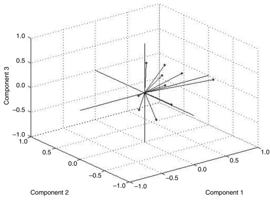
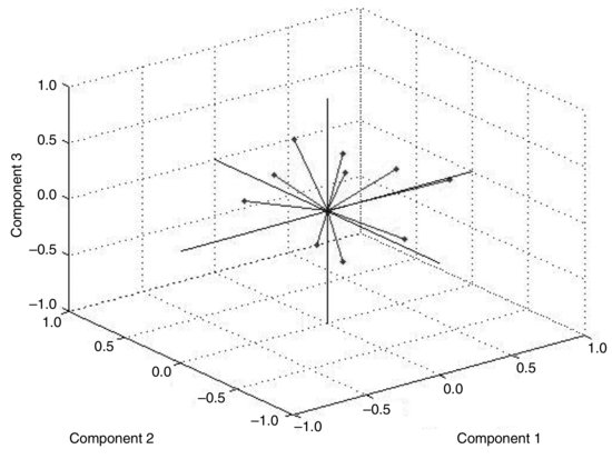
Figure 5 Graphical Representation of Factor Loadings
PCA AND FACTOR ANALYSIS COMPARED
The two illustrations of PCA and FA are relative to the same data and will help clarify the differences between the two methods. Let’s first observe that PCA does not imply, per se, any specific restriction on the process. Given a nonsingular covariance matrix, we can always perform PCA as an exact linear transformation of the series. When we consider a smaller number of principal components, we perform an approximation that has to be empirically justified. For example, in our PCA illustration, the first three components explain 76% of the total variance (based on the covariance matrix; see Table 4).
Factor analysis, on the other hand, assumes that the data have a strict factor structure in the sense that the covariance matrix of the data can be represented as a function of the covariances between factors plus idiosyncratic variances. This assumption has to be verified, otherwise the estimation process might yield incorrect results.
In other words, PCA tends to be a dimensionality reduction technique that can be applied to any multivariate distribution and that yields incremental results. This means that there is a trade-off between the gain in estimation from dimensionality reduction and the percentage of variance explained. Consider that PCA is not an estimation procedure: It is an exact linear transformation of a time series. Estimation comes into play when a reduced number of principal components is chosen and each variable is regressed onto these principal components. At this point, a reduced number of principal components yields a simplified regression, which results in a more robust estimation of the covariance matrix of the original series though only a fraction of the variance is explained.
Factor analysis, on the other hand, tends to reveal the exact factor structure of the data. That is, FA tends to give an explanation in terms of what factors explain what processes. Factor rotation can be useful both in the case of PCA and FA. Consider FA. In our illustration, to make the factor model identifiable, we applied the restriction that factors are orthonormal variables. This restriction, however, might result in a matrix of factor loadings that is difficult to interpret.
For example, if we look at the loading matrix in Table 8, there is no easily recognizable structure, in the sense that the time series is influenced by all factors. Figure 5 shows graphically the relationship of the time series to the factors. In this graphic, each of the 10 time series is represented by its three loadings.
We can try to obtain a better representation through factor rotation. The objective is to create factors such that each series has only one large loading and thus is associated primarily with one factor. Several procedures have been proposed for doing so. For example, if we rotate factors using the “promax” method, we obtain factors that are no longer orthogonal but that often have a better explanatory power. Figure 6 shows graphically the relationship of time series to the factors after rotation. The association of the series to a factor is more evident. This fact can be seen from the matrix of new factor loadings in Table 9, which shows how nearly each stock has one large loading.
Table 9 Factor Loadings after Rotation
Figure 6 Relationship of Time Series to the Factors after Rotation
KEY POINTS
- Principal component analysis (PCA) and factor analysis are statistical tools used in financial modeling to reduce the number of variables in a model (i.e., to reduce the dimensionality) and to identify a structure in the relationships between variables.
- Factor models seek to explain complex phenomena via a small number of basic causes or factors. In finance these models are typically applied to time series.
- The objective of a factor model in finance is to explain the behavior of a large number of stochastic processes typically price, returns, or rate processes in terms of a small number of factors (which themselves are stochastic processes). In financial modeling, factor models are needed not only to explain data but to make estimation feasible.
- Linear factor models are regression models. The coefficients are referred to as factor loadings or factor sensitivities, and they represent the influence of a factor on some variable.
- Principal components analysis is a tool to determine factors with statistical learning techniques when factors are not exogenously given. PCA implements a dimensionality reduction of a set of observations.
- Performing PCA is equivalent to determining the eigenvalues and eigenvectors of the covariance matrix or of the correlation matrix.
- Factor analysis is an alternative technique for determining factors. The estimation procedure is performed in two steps: (1) estimate the covariance matrix and the factor loadings, and (2) estimate factors using the covariance matrix and the factor loadings.
- The covariance matrix can be estimated with maximum likelihood methods, assuming that the variables are jointly normally distributed and temporally independently and identically distributed. The estimation of models with maximum likelihood methods is not immediate because factors are not observable, and consequently iterative methods such as the expectation maximization (EM) algorithm are generally used.
REFERENCES
Bai, J. (2003). Inferential theory for factor models of large dimensions. Econometrica 71: 135–171.
Bai, J., and Ng, S. (2002). Determining the number of factors in approximate factor models. Econometrica 70: 191–221.
Hendrickson, A. E., and White, P. O. (1964). Promax: A quick method for rotation to orthogonal oblique structure. British Journal of Statistical Psychology 17: 65–70.
Hotelling, H. (1933). Analysis of a complex of statistical variables with principal components. Journal of Educational Psychology 27: 417–441.
Spearman, C. (1904). General intelligence, objectively determined and measured. American Journal of Psychology 15: 201–293.
Thurstone, L. L. (1938). Primary Mental Abilities. Chicago: University of Chicago Press.