
Multifactor Equity Risk Models and Their Applications
Risk management16 is an integral part of the portfolio management process. Risk models are central to this practice, allowing managers to quantify and analyze the risk embedded in their portfolios. Risk models provide managers insight into the major sources of risk in a portfolio, helping them to control their exposures and understand the contributions of different portfolio components to total risk. They help portfolio managers in their decision-making process by providing answers to important questions such as: How does my small-cap exposure affect portfolio risk? Does my underweight in diversified financials hedge my overweight in banks? Risk models are also widely used in various other areas such as in portfolio construction, performance attribution, and scenario analysis.
In this entry, we discuss the structure of multifactor equity risk models, types of factors used in these models, and describe certain estimation techniques. We also illustrate the use of equity risk factor models in various applications, namely the analysis of portfolio risk, portfolio construction, scenario analysis, and performance attribution.
Throughout this entry, we will be using the Barclays Global Risk Model1 for illustration purposes. For completeness, we also refer to other approaches one can take to construct such a model.
MOTIVATION
In this section, we discuss the motivation behind the multifactor equity risk models. Let’s assume that a portfolio manager wants to estimate and analyze the volatility of a large portfolio of stocks. A straightforward idea would be to compute the volatility of the historical returns of the portfolio and use this measure to forecast future volatility. However, this framework does not provide any insight into the relationships between different securities in the portfolio or the major sources of risk. For instance, it does not assist a portfolio manager interested in diversifying her portfolio or constructing a portfolio that has better risk-adjusted performance.
Instead of estimating the portfolio volatility using historical portfolio returns, one could utilize a different strategy. The portfolio return is a function of stock returns and the market weights of these stocks in the portfolio. Using this, the forecasted volatility of the portfolio (σP) can be computed as a function of the weights (w) and the covariance matrix (Σs) of stock returns in the portfolio:
![]()
This covariance matrix can be decomposed into individual stock volatilities and the correlations between stock returns. Volatilities measure the riskiness of individual stock returns and correlations represent the relationships between the returns of different stocks. Looking into these correlations and volatilities, the portfolio manager can gain insight into her portfolio, namely the riskiness of different parts of the portfolio or how the portfolio can be diversified. As we outlined above, to estimate the portfolio volatility we need to estimate the correlation between each pair of stocks. Unfortunately, this means that the number of parameters to be estimated grows quadratically with the number of stocks in the portfolio.2 For most practical portfolios, the relatively large number of stocks makes it difficult to estimate the relationship between stock returns in a robust way. Moreover, this framework uses the history of individual stock returns to forecast future stock volatility. However, stock characteristics are dynamic and hence using returns from different time periods may not produce good forecasts.3 Finally, the analysis does not provide much insight regarding the broad factors influencing the portfolio. These drawbacks constitute the motivation for the multifactor risk models detailed in this entry.
One of the major goals of multifactor risk models is to describe the return of a portfolio using a smaller set of variables, called factors. These factors should be designed to capture broad (systematic) market fluctuations, but should also be able to capture specific nuances of individual portfolios. For instance, a broad U.S. market factor would capture the general movement in the equity market, but not the varying behavior across industries. If our portfolio is heavily biased toward particular industries, the broad U.S. market factor may not allow for a good representation of our portfolio’s return.
In the context of factor models, the total return of a stock is decomposed into a systematic and an idiosyncratic component. Systematic return is the component of total return due to movements in common risk factors, such as industry or size. On the other hand, idiosyncratic return can be described as the residual component that cannot be explained by the systematic factors. Under these models, the idiosyncratic return is uncorrelated across issuers. Therefore, correlations across securities are driven by their exposures to the systematic risk factors and the correlation between those factors.
The following equation demonstrates the systematic and the idiosyncratic components of total stock return:
![]()
The systematic return for security s is the product of the loadings of that security (Ls, also called sensitivities) to the systematic risk factors and the returns of these factors (F). The idiosyncratic return is given by εs. Under these models, the portfolio volatility can be estimated as
![]()
Models represented by equations of this form are called linear factor models. Here Lp represents the loadings of the portfolio to the risk factors (determined as the weighted average of individual stock loadings), and ![]() is the covariance matrix of factor returns. w is the vector of security weights in the portfolio, and Ω is the covariance matrix of idiosyncratic stock returns. Due to the uncorrelated nature of these returns, this covariance matrix is diagonal: all elements outside its diagonal are zero. As a result, the idiosyncratic risk of the portfolio is diversified away as the number of securities in the portfolio increases. This is the diversification benefit attained when combining uncorrelated exposures.
is the covariance matrix of factor returns. w is the vector of security weights in the portfolio, and Ω is the covariance matrix of idiosyncratic stock returns. Due to the uncorrelated nature of these returns, this covariance matrix is diagonal: all elements outside its diagonal are zero. As a result, the idiosyncratic risk of the portfolio is diversified away as the number of securities in the portfolio increases. This is the diversification benefit attained when combining uncorrelated exposures.
For most practical portfolios, the number of factors is significantly smaller than the number of stocks in the portfolio. Therefore, the number of parameters in ![]() is much smaller than in
is much smaller than in ![]() , leading to a generally more robust estimation. Moreover, the factors can be designed in a way that they are relatively more stable than individual stock returns, leading to models with potentially better predictability.
, leading to a generally more robust estimation. Moreover, the factors can be designed in a way that they are relatively more stable than individual stock returns, leading to models with potentially better predictability.
Another important advantage of using linear factor models is the detailed insight they provide into the structure and properties of portfolios. These models characterize stock returns in terms of systematic factors that (can) have intuitive economic interpretations. Linear factor models can provide important insights regarding the major systematic and idiosyncratic sources of risk and return. This analysis can help managers to better understand their portfolios and can guide them through the different tasks they perform, such as rebalancing, hedging, or the tilting of their portfolios. The Barclays Global Risk Model—the model used for illustration throughout this entry—is an example of such a linear factor model.
EQUITY RISK FACTOR MODELS
The design of a linear factor model usually starts with the identification of the major sources of risk embedded in the portfolios of interest. For an equity portfolio manager who invests in various markets across the globe, the major sources of risk are typically country, industry membership, and other fundamental or technical exposures such as size, value, and momentum. The relative significance of these components varies across different regions. For instance, for regional equity risk models in developed markets, industry factors tend to be more important than country factors, although in periods of financial distress country factors become more significant. On the other hand, for emerging markets models the country factor is still considered to be the most important source of risk. For regional models, the relative significance of industry factors depends on the level of financial integration across different local markets in that region. The importance of these factors is also time-varying, depending on the particular time period of the analysis. For instance, country risk used to be a large component of total risk for European equity portfolios. However, country factors have been generally losing their significance in this context due to financial integration in the region as a result of the European Union and a common currency, the euro. This is particularly true for larger European countries. Similarly, the relative importance of industry factors is higher over the course of certain industry-led crises, such as the dot-com bubble burst (2000–2002) and the 2007–2009 banking and credit crisis. As we will see, the relative importance of different risk factors varies also with the particular design and the estimation process chosen to calibrate the model.
A typical global or regional equity risk model has the following structure:
where
ri = the rate of return for stock i
FMKT = the market factor
FIND = the industry factor corresponding to stock i
FCNT = the country factor corresponding to stock i
βi = the exposure (beta) of the stock to the corresponding factor
FFT = the set of fundamental and technical factors
![]() = the loading of stock i to factor FjFT
= the loading of stock i to factor FjFT
εi = the residual return for stock i
There are different ways in which these factors can be incorporated into an equity risk model. The choice of a particular model affects the interpretation of the factors. For instance, consider a model that has only market and industry factors. Industry factors in such a model would represent industry-specific moves net of the market return. On the other hand, if we remove the market factor from the equation, the industry factors now incorporate the overall market effect. Their interpretation would change, with their returns now being close to market value-weighted industry indexes. Country-specific risk models are a special case of the previous representation where the country factor disappears and the market factor is represented by the returns of the countrywide market. Macroeconomic factors are also used in some equity risk models, as discussed later.
The choice of estimation process also influences the interpretation of the factors. As an example, consider a model that has only industry and country factors. These factors can be estimated jointly in one step. In this case, both factors represent their own effect net of the other ones. On the other hand, these factors can be estimated in a multistep process—e.g., industry factors estimated in the first step and then the country factors estimated in the second step, using residual returns from the first step. In this case, the industry factors have an interpretation close to the market value-weighted industry index returns, while the country factors would now represent a residual country average effect, net of industry returns. We discuss this issue in more detail in the following section.
Model Estimation
In terms of the estimation methodology, there are three major types of multi-factor equity risk models: cross-sectional, time series, and statistical. All three of these methodologies are widely used to construct linear factor models in the equity space.4 In cross-sectional models, loadings are known and factors are estimated. Examples of loadings used in these models are industry membership variables and fundamental security characteristics (e.g., the book-to-price ratio). Individual stock returns are regressed against these security-level loadings in every period, delivering estimation of factor returns for that period. The interpretation of these estimated factors is usually intuitive, although dependent on the estimation procedure and on the quality of the loadings. In time-series models, factors are known and loadings are estimated. Examples of factors in these models are financial or macroeconomic variables, such as market returns or industrial production. Time series of individual equity returns are regressed against the factor returns, delivering empirical sensitivities (loadings or betas) of each stock to the risk factors. In these models, factors are constructed and not estimated, therefore, their interpretation is straightforward. In statistical models (e.g., principal component analysis), both factors and loadings are estimated jointly in an iterative fashion. The resulting factors are statistical in nature, not designed to be intuitive. That being said, a small set of the statistical factors can be (and usually are) correlated with broad economic factors, such as the market. Table 1 summarizes some of the characteristics of these models.
Table 1 Cross-Sectional, Time-Series, and Statistical Factor Models
An important advantage of cross-sectional models is that the number of parameters to be estimated is generally significantly smaller as compared to the other two types of models. On the other hand, cross-sectional models require a much larger set of input data (company-specific loadings). Cross-sectional models tend to be relatively more responsive as loadings can adjust faster to changing market conditions. There are also hybrid models, which combine cross-sectional and time-series estimation in an iterative fashion; these models allow the combination of observed and estimated factors. Finally, statistical models require only a history of security returns as input to the process. They tend to work better when economic sources of risk are hard to identify and are primarily used in high-frequency applications.
As we mentioned in the previous section, the estimation process is a major determinant in the interpretation of factors. Estimating all factors jointly in one-step regression allows for a natural decomposition of total variance in stock returns. However it also complicates the interpretation of factors as each factor now represents its own effect net of all other factors. Moreover, multicollinearity problems arise naturally in this set-up, potentially delivering lack of robustness to the estimation procedure and leading to unintuitive factor realizations. This problem can be serious when using factors that are highly correlated.
An alternative in this case is to use a multistep estimation process where different sets of factors are estimated sequentially, in separate regressions. In the first step, stock returns are used in a regression to estimate a certain set of factors, and then residual returns from this step are used to estimate the second step factors, and so on. The choice of the order of factors in such estimation influences the nature of the factors and their realizations. This choice should be guided by the significance and the desired interpretation of the resulting factors. The first-step factors have the most straightforward interpretation as they are estimated in isolation from all other factors using raw stock returns. For instance, in a country-specific equity risk model where there are industry, fundamental and technical factors, the return series of industry factors would be close to the industry index returns if they are estimated in isolation in the first step. This would not be the case if all industry, fundamental, and technical factors are estimated in the same step.
An important input to the model estimation is the security weights used in the regressions. There is a variety of techniques employed in practice but generally more weight is assigned to less volatile stocks (usually represented by larger companies). This enhances the robustness of the factor estimates as stocks from these companies tend to have relatively more stable return distributions.
Types of Factors
In this section, we analyze in more detail the different types of factors typically used in equity risk models. These can be classified under five major categories: market factors, classification variables, firm characteristics, macroeconomic variables, and statistical factors.
Market Factors
A market factor can be used as an observed factor in a time-series setting (e.g., in the capital asset pricing model, the market factor is the only systematic factor driving returns). As an example, for a U.S. equity factor model, S&P 500 can be used as a market factor and the loading to this factor—market beta—can be estimated by regressing individual stock returns to the S&P 500. On the other hand, in a cross-sectional setting, the market factor can be estimated by regressing stock returns to their market beta for each time period (this beta can be empirical—estimated via statistical techniques—or set as a dummy loading, usually 1). When incorporated into a cross-sectional regression with other factors, it generally works as an intercept, capturing the broad average return for that period. This changes the interpretation of all other factors to returns relative to that average (e.g., industry factor returns would now represent industry-specific moves net of market).
Classification Variables
Industry and country are the most widely used classification variables in equity risk models. They can be used as observed factors in time-series models via country/industry indexes (e.g., return series of GICS indexes5 can be used as observed industry factors). In a cross-sectional setting, these factors are estimated by regressing stock returns to industry/country betas (either estimated or represented as a 0/1 dummy loading). These factors constitute a significant part of total risk for a majority of equity portfolios, especially for portfolios tilted toward specific industries or countries.
Firm Characteristics
Factors that represent firm characteristics can be classified as either fundamental or technical factors. These factors are extensively used in equity risk models; exposures to these factors represent tilts towards major investment themes such as size, value, and momentum. Fundamental factors generally employ a mix of accounting and market variables (e.g., accounting ratios) and technical factors commonly use return and volume data (e.g., price momentum or average daily volume traded).
In a time-series setting, these factors can be constructed as representative long-short portfolios (e.g., Fama-French factors). As an example, the value factor can be constructed by taking a long position in stocks that have a large book to price ratio and a short position in the stocks that have a small book to price ratio. On the other hand, in a cross-sectional setup, these factors can be estimated by regressing the stock returns to observed firm characteristics. For instance, a book to price factor can be estimated by regressing stock returns to the book to price ratios of the companies. In practice, fundamental and technical factors are generally estimated jointly in a multivariate setting.
A popular technique in the cross-sectional setting is the standardization of the characteristic used as loading such that it has a mean of zero and a standard deviation of one. This implies that the loading to the corresponding factor is expressed in relative terms, making the exposures more comparable across the different fundamental/technical factors. Also, similar characteristics can be combined to form a risk index and then this index can be used to estimate the relevant factor (e.g., different value ratios such as earnings to price and book to price can be combined to construct a value index, which would be the exposure to the value factor). The construction of an index from similar characteristics can help reduce the problem of multicollinearity referred to above. Unfortunately, it can also dilute the signal each characteristic has, potentially reducing its explanatory power. This trade-off should be taken into account while constructing the model. The construction of fundamental factors and their loadings requires careful handling of accounting data. These factors tend to become more significant for portfolios that are hedged with respect to the market or industry exposures.
Macroeconomic Variables
Macroeconomic factors, representing the state of the economy, are generally used as observed factors in time-series models. Widely used examples include interest rates, commodity indexes, and market volatility (e.g., the VIX index). These factors tend to be better suited for models with a long horizon. For short to medium horizons, they tend to be relatively insignificant when included in a model that incorporates other standard factors such as industry. The opposite is not true, suggesting that macro factors are relatively less important for these horizons. This does not mean that the macro-economic variables are not relevant in explaining stock returns; it means that a large majority of macroeconomic effects can be captured through the industry factors. Moreover, it is difficult to directly estimate stock sensitivities to slow-moving macroeconomic variables. These considerations lead to the relatively infrequent use of macro variables in short to medium horizon risk models.6
Statistical Factors
Statistical factors are very different in nature from all the aforementioned factors as they do not have direct economic interpretation. They are estimated using statistical techniques such as principal component analysis where both factors and loadings are estimated jointly in an iterative fashion. Their interpretation can be difficult, yet in certain cases they can be re-mapped to well-known factors. For instance, in a principal component analysis model for the U.S. equity market, the first principal component would represent the U.S. market factor. These models tend to have a relatively high in-sample explanatory power with a small set of factors and the marginal contribution of each factor tends to diminish significantly after the first few factors. Statistical factors can also be used to capture the residual risk in a model with economic factors. These factors tend to work better when there are unidentified sources of risk such as in the case of high-frequency models.
Other Considerations in Factor Models
Various quantitative and qualitative measures can be employed to evaluate the relative performance of different model designs. Generically, better risk models are able to forecast more accurately the risk of different types of portfolios across different economic environments. Moreover, a better model allows for an intuitive analysis of the portfolio risk along the directions used to construct and manage the portfolio. The relative importance of these considerations should frame how we evaluate different models.
A particular model is defined by its estimation framework and the selection of its factors and loadings. Typically, these choices are evaluated jointly, as the contributions of specific components are difficult to measure in practice. Moreover, decisions on one of these components (partially) determine the choice of the others. For instance, if a model uses fundamental firm characteristics as loadings, it also uses estimated factors—more generally, decisions on the nature of the factors determine the nature of the loadings and vice-versa.
Quantitative measures of factor selection include the explanatory power or significance of the factor, predictability of the distribution of the factor, and correlations between factors. On a more qualitative perspective, portfolio managers usually look for models with factors and loadings that have clean and intuitive interpretation, factors that correspond to the way they think about the asset class, and models that reflect their investment characteristics (e.g., short vs. long horizon, local vs. global investors).
Idiosyncratic Risk
Once all systematic factors and loadings are estimated, the residual return can be computed as the component of total stock return that cannot be explained by the systematic factors. Idiosyncratic return—also called residual, nonsystematic, or name-specific return—can be a significant component of total return for individual stocks, but tends to become smaller for portfolios of stocks as the number of stocks increases and concentration decreases (the aforementioned diversification effect). The major input to the computation of idiosyncratic risk is the set of historical idiosyncratic returns of the stock. Because the nature of the company may change fast, a good idiosyncratic risk model should use only recent and relevant idiosyncratic returns. Moreover, recent research suggests that there are other conditional variables that may help improve the accuracy of idiosyncratic risk estimates. For instance, there is substantial evidence that the market value of a company is highly correlated with its idiosyncratic risk, where larger companies exhibit relatively smaller idiosyncratic risk. The use of such variables as an extra adjustment factor can improve the accuracy of idiosyncratic risk estimates.
As mentioned before, idiosyncratic returns of different issuers are assumed to be uncorrelated. However, different securities from the same issuer can show a certain level of co-movement, as they are all exposed to specific events affecting their common issuer.
Interestingly, this co-movement is not perfect or static. Certain news can potentially affect the different securities issued by the same company (e.g., equity, bonds, or equity options) in different ways. Moreover, this relationship changes with the particular circumstances of the firm. For instance, returns from securities with claims to the assets of the firm should be more highly correlated if the firm is in distress. A good risk model should be able to capture these phenomena.
APPLICATIONS OF EQUITY RISK MODELS
Multifactor equity risk models are employed in various applications such as the quantitative analysis of portfolio risk, hedging unwanted exposures, portfolio construction, scenario analysis, and performance attribution. In this section we discuss and illustrate some of these applications.
Portfolio managers can be divided broadly into indexers (those that measure their returns relative to a benchmark index) and absolute return managers (typically hedge fund managers). In between stand the enhanced indexers, those that are allowed to deviate from the benchmark index in order to express views, presumably leading to superior returns. All are typically subject to a risk budget that prescribes how much risk they are allowed to take to achieve their objectives: minimize transaction costs and match the index return for the pure indexers, maximize the net return for the enhanced indexers, or maximize absolute return for absolute return managers. In all of these cases, the manager has to merge all her views and constraints into a final portfolio.
The investment process of a typical portfolio manager involves several steps. Given the investment universe and objective, the steps usually consist of portfolio construction, risk prediction, and performance evaluation. These steps are iterated throughout the investment cycle over each rebalancing period. The examples in this section are constructed following these steps. In particular, we start with a discussion on the portfolio construction process for three equity portfolio managers with different goals: The first aims to track a benchmark, the second to build a momentum portfolio, and the third to implement sector views in a portfolio. We conduct these exercises through a risk-based portfolio optimization approach at a monthly rebalancing frequency. For the index-tracking portfolio example, we then conduct a careful evaluation of its risk exposures and contributions to ensure that the portfolio manager’s views and intuition coincide with the actual portfolio exposures. Once comfortable with the positions and the associated risk, the portfolio is implemented. At the end of the monthly investment cycle, the performance of the portfolio and return contributions of its different components can be evaluated using performance attribution.
Scenario analysis can be employed in both the portfolio construction and the risk evaluation phases of the portfolio process. This exercise allows the manager to gain additional intuition regarding the exposures of her portfolio and how it may behave under particular economic circumstances. It usually takes the form of stress testing the portfolio under historical or hypothetical scenarios. It can also reveal the sensitivity of the portfolio to particular movements in economic and financial variables not explicitly considered during the portfolio construction process. The last application in this entry illustrates this kind of analysis.
Throughout our discussion, we use a suite of global cash equity risk models available through POINT®, the Barclays portfolio analytics and modeling platform.7
Portfolio Construction
Broadly speaking there are two main approaches to portfolio construction: a formal quantitative optimization-based approach and a qualitative approach that is based primarily on manager intuition and skill. There are many variations within and between these two approaches. In this section, we focus on risk-based optimization using a linear factor model. We do not discuss other more qualitative or nonrisk-based approaches (e.g., a stratified sampling). A common objective in a risk-based optimization exercise is the minimization of volatility of the portfolio, either in isolation or when evaluated against a benchmark. In the context of multifactor risk models, total volatility is composed of a systematic and an idiosyncratic component, as described above. Typically, both of these components are used in the objective function of the optimization problems. We demonstrate three different portfolio construction exercises and discuss how equity factor models are employed in this endeavor. The examples were constructed using the POINT® Optimizer.8 All optimization problems were run as of July 30, 2010.
Tracking an Index
In our first example, we study the case of a portfolio manager whose goal is to create a portfolio that tracks a benchmark equity index as closely as possible, using a limited number of stocks. This is a very common problem in the investment industry since most assets under management are benchmarked to broad market indexes. Creating a benchmark-tracking portfolio provides a good starting point for implementing strategic views relative to that benchmark. For example, a portfolio manager might have a mandate to outperform a benchmark under particular risk constraints. One way to implement this mandate is to dynamically tilt the tracking portfolio toward certain investment styles based on views on the future performance of those styles at a particular point in the business cycle.
Consider a portfolio manager who is benchmarked to the S&P 500 index and aims to build a tracking portfolio composed of long-only positions from the set of S&P 500 stocks. Because of transaction cost and position management limitations, the portfolio manager is restricted to a maximum number of 50 stocks in the tracking portfolio. Her objective is to minimize the tracking error volatility (TEV) between her portfolio and the benchmark. Tracking error volatility can be described as the volatility of the return differential between the portfolio and the benchmark (i.e., measures a typical movement in this net position). A portfolio’s TEV is commonly referred to as the risk or the (net) volatility of the portfolio.
As mentioned before, the total TEV is decomposed into a systematic TEV and an idiosyncratic TEV. Moreover, because these two components are assumed to be independent,
![]()
The minimization of systematic TEV is achieved by setting the portfolio’s factor exposures (net of benchmark) as close to zero as possible, while respecting other potential constraints of the problem (e.g., maximum number of 50 securities in the portfolio). The minimization of idiosyncratic volatility is achieved through the diversification of the portfolio holdings.
Table 2 illustrates the total risk for portfolio versus benchmark that comes out of the optimization problem. We see that total TEV of the net position is 39.6 bps/month with 16.9 bps/month of systematic TEV and 35.8 bps/month of idiosyncratic TEV. If the portfolio manager wants to reduce her exposure to name-specific risk, she can increase the upper bound on the number of securities picked by the optimizer to construct the optimal portfolio (increasing the diversification effect). Another option would be to increase the relative weight of idiosyncratic TEV compared to the systematic TEV in the objective function. The portfolio resulting from this exercise would have smaller idiosyncratic risk but, unfortunately, would also have higher systematic risk. This trade-off can be managed based on the portfolio manager’s preferences.
Table 2 Total Risk of Index-Tracking Portfolio vs. the Benchmark (bps/month)
| Attribute | Realized Value |
| Total TEV | 39.6 |
| Idiosyncratic TEV | 35.8 |
| Systematic TEV | 16.9 |
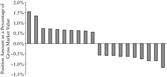
Figure 1 Position Amount of Individual Stocks in the Optimal Tracking Portfolio
Table 3 Largest Risk Factor Exposures for the Momentum Winners/Losers Portfolio (bps/month)
Figure 1 depicts the distribution of the position amount for individual stocks in the portfolio. We can see that the portfolio is well diversified across the 50 constituent stocks with no significant concentrations in any of the individual positions. The largest stock position is 4.1%, about three times larger than the smallest holding. Later in this entry, we analyze the risk of this particular portfolio in more detail.
Constructing a Factor-Mimicking Portfolio
Factor-mimicking portfolios allow portfolio managers to capitalize on their views on various investment themes. For instance, the portfolio manager may forecast that small-cap stocks will outperform large-cap stocks or that value stocks will outperform growth stocks in the near future. By constructing long-short factor-mimicking portfolios, managers can place positions in line with their views on these investment themes without taking explicit directional views on the broader market.
Considering another example, suppose our portfolio manager forecasts that recent winner (high momentum) stocks will outperform recent losers (low momentum). To implement her views, she constructs two portfolios, one with winner stocks and one with loser stocks (100 stocks from the S&P 500 universe in each portfolio). She then takes a long position in the winners portfolio and a short position in the losers portfolio. While a sensible approach, a long-short portfolio constructed in this way would certainly have exposures to risk factors other than momentum. For instance, the momentum view might implicitly lead to unintended sector bets. If the portfolio manager wants to understand and potentially limit or avoid these exposures, she needs to perform further analysis. The use of a risk model will help her substantially.
Figure 2 Largest 10 Positions on Long and Short Sides for the Momentum Portfolio
To illustrate this point, table 3 shows one of POINT®’s risk model outputs—the 10 largest risk factor exposures by their contribution to TEV (last column in the table) for the initial long-short portfolio. While momentum has the largest contribution to volatility, other risk factors also play a significant role. As a result, major moves in risk factors other than momentum can have a significant—and potentially unintended—impact on the portfolio’s return.
Given this information, suppose our portfolio manager decides to avoid these exposures to the extent possible. She can do that by setting all exposures to factors other than momentum to zero (these type of constraints may not always be feasible and one may need to relax them to achieve a solution). Moreover, because she wants the portfolio to represent a pure systematic momentum effect, she seeks to minimize idiosyncratic risk. There are many ways to implement these additional goals, but increasingly portfolio managers are turning to risk models (using an optimization engine) to construct their portfolios in a robust and convenient way. She decides to set up an optimization problem where the objective function is the minimization of idiosyncratic risk. The tradable universe is the set of S&P 500 stocks and the portfolio is constructed to be dollar-neutral. This problem also incorporates the aforementioned factor exposure constraints.
The resulting portfolio (not shown) has exactly the risk factor exposures that were specified in the problem constraints. It exhibits a relatively low idiosyncratic TEV. Figure 2 depicts the largest 10 positions on the long and short sides of the momentum factor-mimicking portfolio; we see that there are no significant individual stock concentrations.
Implementing Sector Views
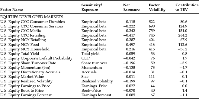
For our final portfolio construction example, let’s assume we are entering a recessionary environment. An equity portfolio manager forecasts that the consumer staples sector will outperform the consumer discretionary sector in the near future, so she wants to create a portfolio to capitalize on this view. One simple idea would be to take a long position in the consumer staples sector (NCY: noncyclical) and a short position in the consumer discretionary sector (CYC: cyclical) by using, for example, sector ETFs. Similar to the previous example, this could result in exposures to risk factors other than the industry factors. Table 4 illustrates the exposure of this long-short portfolio to the risk factors in the POINT® U.S. equity risk model. As we can see in the table, the portfolio has significant net exposures to certain fundamental and technical factors, such as share turnover.
Table 4 Factor Exposures and Contributions for Consumer Staples vs. Consumer Discretionary Portfolio (bps/month)

Suppose the portfolio manager decides to limit exposures to fundamental and technical factors. We can again use the optimizer to construct a long-short portfolio, with an exposure (beta) of 1 to the consumer staples sector and a beta of −1 to the consumer discretionary sector. To limit the exposure to fundamental and technical risk factors, we further impose the exposure to each of these factors to be between −0.2 and 0.2.9 We also restrict the portfolio to be dollar neutral, and allow for only long positions in the consumer staples stocks and for only short positions in consumer discretionary stocks. Finally, we restrict the investment universe to the members of the S&P 500 index.10
The resulting portfolio consists of 69 securities (approximately half of discretionary and staples stocks in S&P 500) with 31 long positions in the consumer staples stocks and 38 short positions in consumer discretionary stocks. Table 5 depicts the factor exposures for this portfolio. As we can see in the table, the sum of the exposures to the industry factors is 1 for the consumer staples stocks and −1 for the consumer discretionary stocks. Exposures to fundamental and technical factors are generally significantly smaller when compared to the previous table, limiting the adverse effects of potential moves in these factors. Interestingly, no stocks from the automobiles industry are selected in the optimal portfolio, potentially due to excessive idiosyncratic risk of firms in that particular industry. The contribution to volatility from the cyclical sector is higher than that from the non-cyclical sector, due to higher volatility of industry factors in the former.
Table 5 Factor Exposures and Contributions for the Optimal Sector View Portfolio (bps/month)
The bounds used for the fundamental and technical factor exposures in the portfolio construction process were set to force a reduction in the exposure to these factors. However, there is a trade-off between having smaller exposures and having smaller idiosyncratic risk in the final portfolio. The resolution of this trade-off depends on the preferences of the portfolio manager. When the bounds are more restrictive, we are also decreasing the feasible set of solutions available to the problem and therefore potentially achieving a higher idiosyncratic risk (remember that the objective is the minimization of idiosyncratic risk). In our example, the idiosyncratic TEV of the portfolio increases from 119 bps/month (before the optimization) to 158 bps/month on the optimized portfolio. This change is the price paid for the ability to limit certain systematic risk factor exposures.
Analyzing Portfolio Risk Using Multifactor Models
Now that we have seen examples of using multifactor equity models for portfolio construction and briefly discussed their risk outcomes, we take a more in-depth look at portfolio risk. Risk analysis based on multifactor models can take many forms, from a relatively high-level aggregate approach to an in-depth analysis of the risk properties of individual stocks and groups of stocks. Multifactor equity risk models provide the tools to perform the analysis of portfolio risk in many different dimensions, including exposures to risk factors, security factor contributions to total risk, analysis at the ticker level, and scenario analysis. In this section, we provide an overview of such detailed analysis using the S&P 500 index tracker example we created in the previous section.
Recall from Table 2 that the TEV of the optimized S&P 500 tracking portfolio was 39.6 bps/month, composed mostly of idiosyncratic risk (35.8 bps/month) and a relatively small amount of systematic risk (16.9 bps/month). To analyze further the source of these numbers, we first compare the holdings of the portfolio with those of the benchmark and then study the impact of the mismatch to the risk of the net position (Portfolio–Benchmark). The first column in Table 6 shows the net market weights (NMW) of the portfolio at the sector level (GICS level 1). Our portfolio appears to be well balanced with respect to the benchmark from a net market weight perspective. The largest market value discrepancies are an overweight in information technology (+5.2%) and an underweight in consumer discretionary (−3.6%) and health care (−3.3%) companies. However, the sector with the largest contribution to overall risk (contribution to TEV, or CTEV) is financials (7.5 bps/month). This may seem unexpected, given the small NMW of this sector (0.1%). This result is explained by the fact that contributions to risk (CTEV) are dependent on the net market weight of an exposure, its risk and also the correlation between the different exposures. Looking into the decomposition of the CTEV, the table also shows that most of the total contribution to risk from financials is idiosyncratic (7.0 bps/month). This result is due to the small number of securities our portfolio has in this sector and the underlying high volatility of these stocks. In short, the diversification benefits across financial stocks are small in our portfolio: We could potentially significantly reduce total risk by constructing our financials exposure using more names. Note that this analysis is only possible with a risk model.
Table 6 Net Market Weights and Risk Contributions by Sector (bps/month)

Table 7 Additional Risk Measures by Sector
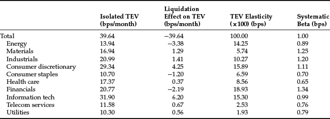
Table 7 highlights additional risk measures by sector. What we see in the first column is the isolated TEV, that is, the risk associated with the stocks in that particular sector only. On an isolated basis, the information technology sector has the highest risk in the portfolio. This top position in terms of isolated risk does not translate into the highest contribution to overall portfolio risk, as we saw in Table 6. The discrepancy between isolated risk numbers and contributions to risk is explained by the correlation between the exposures and allows us to understand the potential hedging effects present across our portfolio. The liquidation effect reported in the table represents the change in TEV when we completely hedge that particular position, that is, enforce zero net exposure to any stock in that particular sector. Interestingly, eliminating our exposure to information technology stocks would actually increase our overall portfolio risk by 6.2 bps/month. This happens because the overweight in this sector is effectively hedging out risk contributions from other sectors. If we eliminate this exposure, the portfolio balance is compromised. The TEV elasticity reported gives an additional perspective regarding how the TEV in the portfolio changes when we change the exposure to that sector. Specifically, it tells us the percentage change in TEV for each 1% change in our exposure to that particular sector. For example, if we double our exposure to the energy sector, our TEV would increase by 14.25% (from 39.6 bps/month to 45.2 bps/month). Finally, the report estimates the portfolio to have a beta of 1.00 to the benchmark, which is, of course, in line with our index tracking objective. The beta statistic measures the comovement between the systematic risk drivers of the portfolio and the benchmark and should be interpreted only as that. In particular, a low portfolio beta (relative to the benchmark) does not imply low portfolio risk. It signals relatively low systematic co-movement between the two universes or a relatively high idiosyncratic risk for the portfolio. For example, if the sources of systematic risk from the portfolio and the benchmark are distinct, the portfolio beta is close to zero. The report also provides the systematic beta associated with each sector. For instance, we see that a movement of 1% in the benchmark leads to a 1.34% return in the financials component of our portfolio. As expected, consumer staples and health care are two low beta industries, as they tend to be more stable through the business cycle.11
Although important, the information we examined so far is still quite aggregated. For instance, we know from Table 6 that a large component of idiosyncratic risk comes from financials. But what names are contributing most? What are the most volatile sectors? How are systematic exposures distributed within each sector? Risk models should be able to provide answers to all these questions, allowing for a detailed view of the portfolio’s risk exposures and contributions. As an example, Table 8 displays all systematic risk factors the portfolio or the benchmark loads onto. It also provides the portfolio, benchmark, and net exposures for each risk factor, the volatility of each of these factors, and their contributions to total TEV. The table shows that the net exposures to the risk factors are generally low, meaning that the tracking portfolio has small active exposures. This finding is in line with the evidence from Table 2, where we see that the systematic risk is small (16.9 bps/month). If we look into the contributions of individual factors to total TEV, the table shows that the top contributors are the size, share turnover, and realized volatility factors. The optimal index tracking portfolio tends to be composed of very large-cap names within the specified universe, and that explains the net positive loading to the market value (size) factor. This portfolio tilt is due to the generally low idiosyncratic risk large companies have. This is seen favorably by the optimization engine, as it tries to minimize idiosyncratic risk. This same tilt would explain our net exposure to both the share turnover and realized volatility factors, as larger companies tend to have lower realized volatility and share turnover too. Interestingly, industry factors have relatively small contributions to TEV, even though they exhibit significantly higher volatilities. This results from the fact that the optimization engine specifically targets these factors because of their high volatility and is successful in minimizing net exposure to industry factors in the final portfolio.
Table 8 Factor Exposures and Contributions for the Tracking Portfolio vs. S&P 500 (bps/month)
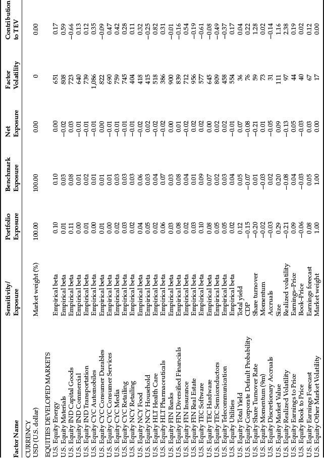
Table 9 Individual Securities and Idiosyncratic Risk Exposures

Finally, remember from Table 2 that the largest component of the portfolio risk comes from name-specific exposures. Therefore, it is important to be aware of which individual stocks in our portfolio contribute the most to overall risk. Table 9 shows the set of stocks in our portfolio with the largest idiosyncratic risk. The portfolio manager can use this information as a screening device to filter out undesirable positions with high idiosyncratic risk and to make sure her views on individual firms translate into risk as expected. In particular, the list in the table should only include names about which the portfolio manager has strong views, either positive—expressed with positive NMW—or negative—in which case we would expect a short net position.
It should be clear from the above examples that although the factors used to measure risk are predetermined in a linear factor model, there is a large amount of flexibility on the way the risk numbers can be aggregated and reported. Instead of sectors, we could have grouped risk by any other classification of individual stocks, for example, by regions or market capitalization. This allows the risk to be reported using the same investment philosophy underlying the portfolio construction process12 regardless of the underlying factor model. There are also many other risk analytics available, not mentioned in this example, that give additional detail about specific risk properties of the portfolio and the constituents. We have only discussed total, systematic, and idiosyncratic risk (which can be decomposed into risk contributions on a flexible basis), and referred to isolated and liquidation TEV, TEV elasticity, and portfolio beta. Most users of multifactor risk models will find their own preferred approach to risk analysis through experience.
Performance Attribution
Now that we discussed portfolio construction and risk analysis as the first steps of the investment process, we give a brief overview of performance attribution, an ex post analysis of performance typically conducted at the end of the investment horizon. Performance attribution analysis provides an evaluation of the portfolio manager’s performance with respect to various decisions made throughout the investment process. The underperformance or outperformance of the portfolio manager when compared to the benchmark can be due to different reasons, including effective sector allocation, security selection, or tilting the portfolio toward certain risk factors. Attribution analysis aims to unravel the major sources of this performance differential. The exercise allows the portfolio manager to understand how her particular views—translated into net exposures—performed during the period and reveals whether some of the portfolio’s performance was the result of unintended bets.
There are three basic forms of attribution analysis used for equity portfolios. These are return decomposition, factor model–based attribution, and style analysis. In the return decomposition approach, the performance of the portfolio manager is generally attributed to top-down allocation (e.g., currency, country, or sector allocation) in a first step, followed by a bottom-up security selection performance analysis. This is a widely used technique among equity portfolio managers.
Factor model–based analysis attributes performance to exposures to risk factors such as industry, size, and financial ratios. It is relatively more complicated than the previous approach and is based on a particular risk model that needs to be well understood. For example, let’s assume that a portfolio manager forecasts that value stocks will outperform growth stocks in the near future. As a result, the manager tilts the portfolio toward value stocks as compared to the benchmark, creating an active exposure to the value factor. In an attribution framework without systematic factors, such sources of performance cannot be identified and hence may be inadvertently attributed to other reasons. Factor model–based attribution analysis adds value by incorporating these factors (representing major investment themes) explicitly into the return decomposition process and by identifying additional sources of performance represented as active exposures to systematic risk factors.
Style analysis, on the other hand, is based on a regression of the portfolio return to a set of style benchmarks. It requires very little information (e.g., we do not need to know the contents of the portfolio), but the outcome depends significantly on the selection of style benchmarks. It also assumes constant loadings to these styles across the regression period, which may be unrealistic for managers with somewhat dynamic allocations.
Factor–Based Scenario Analysis
The last application we review goes over the use of equity risk factor models in the context of scenario analysis. Many investment professionals utilize scenario analysis in different shapes and forms for both risk and portfolio construction purposes. Factor-based scenario analysis is a tool that helps portfolio managers in their decision-making process by providing additional intuition on the behavior of their portfolio under a specified scenario. A scenario can be a historical episode, such as the equity market crash of 1987, the war in Iraq, or the 2008 credit crisis. Alternatively, scenarios can be defined as a collection of hypothetical views (e.g., user-defined scenarios) in a variety of forms such as a view on a given portfolio or index (e.g., S&P 500 drops by 20%) or a factor (e.g., U.S. equity–size factor moves by 3 standard deviations) or correlation between factors (e.g., increasing correlations across markets in episodes of flight to quality). In this section, we use the POINT® Factor-Based Scenario Analysis Tool to illustrate how we can utilize factor models to perform scenario analysis.
Table 10 Index Returns under Scenario 1 (VIX jumps by 50%)
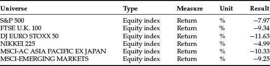
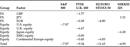
Table 11 Return Contributions for Equity Indexes under Scenario 1 (in %)
Before we start describing the example, let’s take an overview of the mechanics of the model. It allows for the specification of user views on returns of portfolios, indexes, or risk factors. When the user specifies a view on a portfolio or index, this is translated into a view on risk factor realizations, through the linear factor model framework.13 These views are combined with ones that are directly specified in terms of risk factors. It is important to note that the portfolio manager does not need to specify views on all risk factors, and typically has views only on a small subset of them. Once the manager specifies this subset of original views, the next step is to expand these views to the whole set of factors. The scenario analysis engine achieves this by estimating the most likely realization of all other factors—given the factor realizations on which views are specified—using the risk model covariance matrix. Once all factor realizations are populated, the scenario outcome for any portfolio or index can be computed by multiplying their specific exposures to the risk factors by the factor realizations under the scenario. The tool provides a detailed analysis of the portfolio behavior under the specified scenario.
We illustrate this tool using two different scenarios: a 50% shift in the U.S. equity market volatility—represented by the VIX index—(scenario 1) and a 50% jump in the European credit spreads (scenario 2).14 We use a set of equity indexes from across the globe to illustrate the impact of these two scenarios. We run the scenarios as of July 30, 2010, which specifies the date both for the index loadings and the covariance matrix used. Base currency is set to U.S. dollars (USD) and hence index returns presented below are in USD.
Table 10 shows the returns of the chosen equity indexes under the first scenario. We see that all indexes experience significant negative returns with Euro Stoxx plummeting the most and Nikkei experiencing the smallest drop. To understand these numbers better, let’s look into the contributions of different factors to these index returns.
Table 11 illustrates return contributions for four of these equity indexes under scenario 1. Specifically, for each index, it decomposes the total scenario return into return coming from different factors each index has exposure to. In this example, all currency factors are defined with respect to USD. Moreover, equity factors are expressed in their corresponding local currencies and can be described as broad market factors for their respective regions.
Table 12 Factor Returns and Z-Scores under Scenario 1
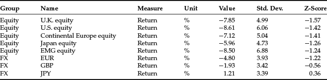
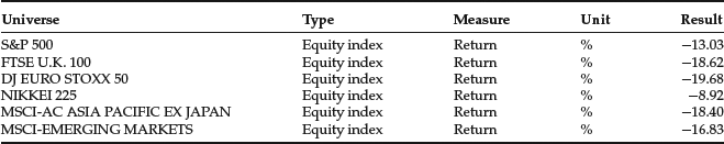
Table 13 Index Returns under Scenario 2 (EUR Credit Spread Jumps by 50%)
Not surprisingly, Table 11 shows that the majority of the return contributions for selected indexes come from the reaction of equity market factors to the scenario. However, foreign exchange (FX) can also be a significant portion of total return for some indexes, such as in the case of the Euro Stoxx (−4.8%). Nikkei experiences a relatively smaller drop in USD terms, majorly due to a positive contribution coming from the JPY FX factor. This positive contribution is due to the safe haven nature of Japanese yen in case of flight to quality under increased risk aversion in global markets.
Table 12 demonstrates the scenario-implied factor realizations (“value”), factor volatilities, and the Z-scores for the risk factors given in Table 11. The Z-score of the factor quantifies the effect of the scenario on that specific factor. It is computed as
![]()
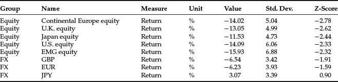
where r is the return of the factor in the scenario and σr is the standard deviation of the factor. Hence, the Z-score measures how many standard deviations a factor moves in a given scenario. Table 12 lists the factors by increasing Z-score under scenario 1. The U.K. equity factor experiences the largest negative move, at −1.57 standard deviations. FX factors experience relatively smaller movements. JPY is the only factor with a positive realization due to the aforementioned characteristic of the currency.
In the second scenario, we shift European credit spreads by 50% (a 3.5-sigma event) and explore the effect of credit market swings on the equity markets. As we can see in Table 13, all equity indexes experience significant returns, in line with the severity of the scenario.15 The result also underpins the strong recent co-movement between the credit and equity markets. The exception is again the Nikkei that realizes a relatively smaller return.
Table 14 provides the return, volatility, and the Z-score of certain relevant factors under scenario 2. As expected, the major mover on the equity side is the continental Europe equity factor, followed by the United Kingdom. Given the recent strong correlations between equity and credit markets across the globe, the table suggests that a 3.5 standard deviation shift in the European spread factor results in a 2 to 3 standard deviation movement of global equity factors.
Table 14 Factor Returns and Z-Scores under Scenario 2
The two examples above illustrate the use of factor models in performing scenario analysis to achieve a clear understanding of how a portfolio may react under different circumstances.
KEY POINTS
- Multifactor equity risk models provide detailed insight into the structure and properties of portfolios. These models characterize stock returns in terms of systematic factors and an idiosyncratic component. Systematic factors are generally designed to have intuitive economic interpretation and they represent common movements across securities. On the other hand, the idiosyncratic component represents the residual return due to stock-specific events.
- Systematic factors used in equity risk models can be broadly classified under five categories: market factors, classification variables, firm characteristics, macroeconomic variables, and statistical factors.
- Relative significance of systematic risk factors depends on various parameters such as the model horizon, region/country for which the model is designed, existence of other factors, and the particular time period of the analysis. For instance, in the presence of industry factors, macroeconomic factors tend to be insignificant for short to medium horizon equity risk models whereas they tend to be more significant for long-horizon models. Moreover, for developed equity markets, industry factors are typically more significant as compared to the country factors. The latter are still the dominant effect for emerging markets.
- Choice of the model and the estimation technique affect the interpretation of factors. For instance, in the existence of a market factor, industry factors represent industry-specific movements net of market. If there is no market factor, their interpretation is very close to market value-weighted industry indexes.
- Multifactor equity risk models can be classified according to how their loadings and factors are specified. The most common equity factor models specify loadings based on classification (e.g., industry) and fundamental or technical information, and estimate factor realizations every period. Certain other models take factors as known (e.g., returns on industry indexes) and estimate loadings based on time-series information. A third class of models is based purely on statistical approaches without concern for economic interpretation of factors and loadings. Finally, it is possible to combine these approaches and construct hybrid models. Each of these approaches has its own specific strengths and weaknesses.
- A good multifactor equity risk model provides detailed information regarding the exposures of a complex portfolio and can be a valuable tool for portfolio construction and risk management. It can help managers construct portfolios tracking a particular benchmark, express views subject to a given risk budget, and rebalance a portfolio while avoiding excessive transaction costs. Further, by identifying the exposures where the portfolio has the highest risk sensitivity it can help a portfolio manager reduce (or increase) risk in the most effective way.
- Performance attribution based on multifactor equity risk models can give ex post insight into how the portfolio manager’s views and corresponding investments translated into actual returns.
- Factor-based scenario analysis provides portfolio managers with a powerful tool to perform stress testing of portfolio positions and gain insight into the impact of specific market events on portfolio performance.
NOTES
1. The Barclays Global Risk Model is available through POINT®, Barclays portfolio management tool. It is a multicurrency cross-asset model that covers many different asset classes across the fixed income and equity markets, including derivatives in these markets. At the heart of the model is a covariance matrix of risk factors. The model has more than 500 factors, many specific to a particular asset class. The asset class models are periodically reviewed. Structure is imposed to increase the robustness of the estimation of such a large covariance matrix. The model is estimated from historical data. It is calibrated using extensive security-level historical data and is updated on a monthly basis.
2. As an example, if the portfolio has 10 stocks, we need to estimate 45 parameters, with 100 stocks we would need to estimate 4,950 parameters.
3. This is especially the case over crisis periods where stock characteristics can change dramatically over very short periods of time.
4. Fixed income managers typically use cross-sectional type of models.
5. GICS is the Global Industry Classification Standard by Standard & Poor’s, a widely used classification scheme by equity portfolio managers.
6. An application of macro variables in the context of risk factor models is as follows. First, we get the sensitivities of the portfolio to the model’s risk factors. Then we project the risk factors into the macro variables. We then combine the results from these two steps to get the indirect loadings of the portfolio to the macro factors. Therefore, instead of calculating the portfolio sensitivities to macro factors by aggregating individual stock macro sensitivities—that are always hard to estimate—we work with the portfolio’s macro loadings, estimated indirectly from the portfolio’s risk factor loadings as described above. This indirect approach may lead to statistically more robust relationships between portfolio returns and macro variables.
7. The equity risk model suite in POINT consists of six separate models across the globe: the United States, United Kingdom, Continental Europe, Japan, Asia (excluding Japan), and global emerging markets equity risk models (for details see Silva, Staal, and Ural, 2009). It incorporates many unique features related to factor choice, industry and fundamental exposures, and risk prediction.
8. See Kumar (2010).
9. The setting of these exposures and its trade-offs are discussed later in this entry.
10. As POINT® U.S. equity risk model incorporates industry level factors, a unit exposure to a sector is implemented by restricting exposures to different industries within that sector to sum up to 1. Also, note that as before, the objective in the optimization problem is the minimization of idiosyncratic TEV to ensure that the resulting portfolio represents systematic—not idiosyncratic—effects.
11. Note that we can sum the sector betas into the portfolio beta, using portfolio sector weights (not net weights) as weights in the summation.
12. For a detailed methodology on how to perform this customized analysis, see Silva (2009).
13. Specifically, we can back out factor realizations from the portfolio or index returns by using their risk factor loadings.
14. For reference, as of July 30, 2010, scenario 1 would imply the VIX would move from 23.5 to 35.3 and scenario 2 would imply that the credit spread for the Barclays European Credit Index would change from 174 bps to 261 bps.
15. The same scenario results in a −8.12% move in the Barclays Euro Credit Index.
16. The authors would like to thank Andy Sparks, Anuj Kumar, and Chris Sturhahn of Barclays for their help and comments.
REFERENCES
Kumar, A. (2010). The POINT optimizer. Barclays Publication, June.
Silva, A. B. (2009). Risk attribution with custom-defined risk factors. Barclays Publication, August.
Silva, A. B., Staal, A. D., and Ural, C. (2009). The US equity risk model. Barclays Publication, July.