Regression Analysis: Theory and Estimation

SERGIO M. FOCARDI, PhD

Partner, The Intertek Group

FRANK J. FABOZZI, PhD, CFA, CPA

Professor of Finance, EDHEC Business School

Our first basic tool in econometrics is regression analysis. In regression analysis, we estimate the relationship between a random variable Y and one or more variables Xi. The variables Xi can be either deterministic variables or random variables. The variable Y is said to be the dependent variable because its value is assumed to be dependent on the value of the Xi’s. The Xi’s are referred to as the independent variables, regressor variables, or explanatory variables. Our primary focus is on the linear regression model. We will be more precise about what we mean by a “linear” regression model later in this entry. Let’s begin with a discussion of the concept of dependence.

THE CONCEPT OF DEPENDENCE

Regressions are about dependence between variables. In this section we provide a brief discussion of how dependence is represented in both a deterministic setting and a probabilistic setting. In a deterministic setting, the concept of dependence is embodied in the mathematical notion of function. A function is a correspondence between the individuals of a given domain A and the individuals of a given range B. In particular, numerical functions establish a correspondence between numbers in a domain A and numbers in a range B.

In quantitative science, we work with variables obtained through a process of observation or measurement. For example, price is the observation of a transaction, time is the reading of a clock, position is determined with measurements of the coordinates, and so on. In quantitative science, we are interested in numerical functions y = f(x1, … , xn) that link the results of measurements so that by measuring the independent variables (x1, … , xn) we can predict the value of the dependent variable y. Being the results of measurements, variables are themselves functions that link a set of unobserved “states of the world” to observations. Different states of the world result in different values for the variables but the link among the variables remains constant. For example, a column of mercury in a thermometer is a physical object that can be in different “states.” If we measure the length and the temperature of the column (in steady conditions), we observe that the two measurements are linked by a well-defined (approximately linear) function. Thus, by measuring the length, we can predict the temperature.

In order to model uncertainty, we keep the logical structure of variables as real-valued functions defined on a set Ω of unknown states of the world. However, we add to the set Ω the structure of a probability space. A probability space is a triple formed by a set of individuals (the states of the world), a structure of events, and a probability function: (Ω, , P). Random variables represent measurements as in the deterministic case, but with the addition of a probability structure that represents uncertainty. In financial econometrics, a “state of the world” should be intended as a complete history of the underlying economy, not as an instantaneous state.

Our objective is to represent dependence between random variables, as we did in the deterministic case, so that we can infer the value of one variable from the measurement of the other. In particular, we want to infer the future values of variables from present and past observations. The probabilistic structure offers different possibilities. For simplicity, let’s consider only two variables X and Y; our reasoning extends immediately to multiple variables. The first case of interest is the case when the dependent variable Y is a random variable while the independent variable X is deterministic. This situation is typical of an experimental setting where we can fix the conditions of the experiment while the outcome of the experiment is uncertain.

In this case, the dependent variable Y has to be thought of as a family of random variables Yx, all defined on the same probability space (Ω, , P), indexed with the independent variable x. Dependence means that the probability distribution of the dependent random variable depends on the value of the deterministic independent value. To represent this dependence we use the notation F(y|x) to emphasize the fact that x enters as a parameter in the distribution. An obvious example is the dependence of a price random variable on a time variable in a stochastic price process.

In this setting, where the independent variable is deterministic, the distributions F(y|x) can be arbitrarily defined. Important for the discussion of linear regressions in this entry is the case when the shape of the distribution F(y|x) remains constant and only the mean of the distribution changes as a function of x.

Consider now the case where both X and Y are random variables. For example, Y might be the uncertain price of IBM stock tomorrow and X the uncertain level of the S&P 500 tomorrow. One way to express the link between these two variables is through their joint distribution F(x,y) and, if it exists, their joint density f(x,y). We define the joint and marginal distributions as follows:

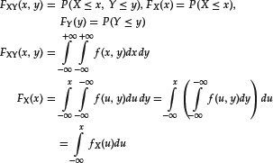
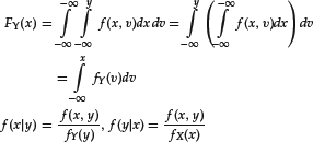
We will also use the short notation:

Given a joint density f(x,y), we can also represent the functional link between the two variables as the dependence of the distribution of one variable on the value assumed by the other variable. In fact, we can write the joint density f(x,y) as the product of two factors, the conditional density f(y|x) and the marginal density fX(x):

(1)

This factorization—that is, expressing a joint density as a product of a marginal density and a conditional density—is the conceptual basis of financial econometrics. There are significant differences in cases where both variables X and Y are random variables, compared to the case where the variable X is deterministic. First, as both variables are uncertain, we cannot fix the value of one variable as if it were independent. We have to adopt a framework of conditioning where our knowledge of one variable influences our knowledge of the other variable.

The impossibility of making experiments is a major issue in econometrics. In the physical sciences, the ability to create the desired experimental setting allows the scientist to isolate the effects of single variables. The experimenter tries to create an environment where the effects of variables other than those under study are minimized. In economics, however, all the variables change together and cannot be controlled. Back in the 1950s, there were serious doubts that econometrics was possible. In fact, it was believed that estimation required the independence of samples while economic samples are never independent.

However, the framework of conditioning addresses this problem. After conditioning, the joint densities of a process are factorized into initial and conditional densities that behave as independent distributions. An econometric model is a probe that extracts independent samples—the noise terms—from highly dependent variables.

Let’s briefly see, at the heuristic level, how conditioning works. Suppose we learn that the random variable X has the value x, that is, X = x. Recall that X is a random variable that is a real-valued function defined over the set Ω. If we know that X = x, we do not know the present state of the world but we do know that it must be in the subspace (ω ∈ Ω: X(ω) = x). We call (Y|X = x) the variable Y defined on this subspace. If we let x vary, we create a family of random variables defined on the family of subspaces (ω ∈ Ω: X(ω) = x) and indexed by the value assumed by the variable X.

It can be demonstrated that the sets (ω ∈ : X(ω) = x) can be given a structure of probability space, that the variables (Y|X = x) are indeed random variables on these probability spaces, and that they have (if they exist) the conditional densities:

(2)

for fX(x) > 0. In the discrete setting we can write

The conditional expectation E[Y|X = x] is the expectation of the variable (Y|X = x). Consider the previous example of the IBM stock price tomorrow and of the S&P 500 level tomorrow. Both variables have unconditional expectations. These are the expectations of IBM’s stock tomorrow and of S&P 500’s level tomorrow considering every possible state of the world. However, we might be interested in computing the expected value of IBM’s stock price tomorrow if we know S&P 500’s value tomorrow. This is the case if, for example, we are creating scenarios based on S&P 500’s value.

If we know the level of the S&P 500, we do not know the present state of the world but we do know the subset of states of the world in which the present state of the world is. If we only know the value of the S&P 500, IBM’s stock price is not known because it is different in each state that belongs to this restricted set. IBM’s stock price is a random variable on this restricted space and we can compute its expected value.

If we consider a discrete setting, that is, if we consider only a discrete set of possible IBM stock prices and S&P 500 values, then the computation of the conditional expectation can be performed using the standard definition of conditional probability. In particular, the conditional expectation of a random variable Y given the event B is equal to the unconditional expectation of the variable Y set to zero outside of B and divided by the probability of B: E[Y|B] = E[1BY]/P(B), where 1B is the indicator function of the set B, equal to 1 for all elements of B, zero elsewhere. Thus, in this example,

However, in a continuous-state setting there is a fundamental difficulty: The set of states of the world corresponding to any given value of the S&P 500 has probability zero; therefore we cannot normalize dividing by P(B). As a consequence we cannot use the standard definition of conditional probability to compute directly the conditional expectation.

To overcome this difficulty, we define the conditional expectation indirectly, using only unconditional expectations. We define the conditional expectation of IBM’s stock price given the S&P 500 level as that variable that has the same unconditional expectation as IBM’s stock price on each set that can be identified by for the value of the S&P 500. This is a random variable which is uniquely defined for each state of the world up to a set of probability zero.

If the conditional density exists, conditional expectation is computed as follows:

(3)

We know from probability theory that the law of iterated expectations holds

(4)

and that the following relationship also holds

(5)

Rigorously proving all these results requires a considerable body of mathematics and the rather difficult language and notation of σ-alge-bras. However, the key ideas should be sufficiently clear.

What is the bearing of the above on the discussion of regressions in this entry? Regressions have a twofold nature: They can be either (1) the representation of dependence in terms of conditional expectations and conditional distributions or (2) the representation of dependence of random variables on deterministic parameters. The above discussion clarifies the probabilistic meaning of both.

REGRESSIONS AND LINEAR MODELS

In this section we discuss regressions and, in particular, linear regressions.

Case Where All Regressors Are Random Variables

Let’s start our discussion of regression with the case where all regressors are random variables. Given a set of random variables X = (Y, X1, … , XN)′, with a joint probability density f(y, x1, … , xN), consider the conditional expectation of Y given the other variables (X1, … , XN)′:

As we saw in the previous section, the conditional expectation is a random variable. We can therefore consider the residual:

The residual is another random variable defined over the set . We can rewrite the above equation as a regression equation:

(6)

The deterministic function y = φ(z) where

(7)

is called the regression function.

The following properties of regression equations hold.

Property 1. The conditional mean of the residual is zero: E[ε|X1, … , XN] = 0. In fact, taking conditional expectations on both sides of equation (7), we can write

Because

is a property that follows from the law of iterated expectations, we can conclude that E[ε|X1, … , XN] = 0.

Property 2. The unconditional mean of the residual is zero: E[ε] = 0. This property follows immediately from the multivariate formulation of the law of iterated expectations (4): E[E[Y|X1, … , XN]] = E[Y]. In fact, taking expectation of both sides of equation (7) we can write

hence E[ε] = 0.

Property 3: The residuals are uncorrelated with the variables X1, … , XN: E[εX] = 0. This follows from equation (6) by multiplying both sides of equation (7) by X1, … , XN and taking expectations. Note however, that the residuals are not necessarily independent of the regressor X.

If the regression function is linear, we can write the following linear regression equation:

(8)

and the following linear regression function:

(9)

The rest of this entry deals with linear regressions. If the vector Z = (Y, X1, … , XN)′ is jointly normally distributed, then the regression function is linear. To see this, partition z, the vector of means μ, and the covariance matrix conformably in the following way:

where μ is the vector of means and Σ is the covariance matrix. It can be demonstrated that the conditional density (Y|X = x) has the following expression:

(10)

where

(11)

The regression function can be written as follows:

(12)

The normal distribution is not the only joint distribution that yields linear regressions. Spherical and elliptical distributions also yield linear regressions. Spherical distributions extend the multivariate normal distribution N(0,I) (i.e., the joint distribution of independent normal variables). Spherical distributions are characterized by the property that their density is constant on a sphere, so that their joint density can be written as

for some function g.

Spherical distributions have the property that their marginal distributions are uncorrelated but not independent, and can be viewed as multivariate normal random variables, with a random covariance matrix. An example of a spherical distribution used in financial econometrics is the multivariate t-distribution with m degrees of freedom, whose density has the following form:

The multivariate t-distribution is important in econometrics for several reasons. First, some sampling distributions are actually a t-distribution entries. Second, the t-distribution proved to be an adequate description of fat-tailed error terms in some econometrics models (although not as good as the stable Paretian distribution).

Elliptical distributions generalize the multivariate normal distribution N(0,Σ). (See Bradley and Taqqu [2003].) Because they are constant on an ellipsoid, their joint density can be written as

where μ is a vector of constants and is a strictly positive-definite matrix. Spherical distributions are a subset of elliptical distributions. Conditional distributions and linear combinations of elliptical distributions are also elliptical.

The fact that elliptical distributions yield linear regressions is closely related to the fact that the linear correlation coefficient is a meaningful measure of dependence only for elliptical distributions. There are distributions that do not factorize as linear regressions. The linear correlation coefficient is not a meaningful measure of dependence for these distributions. The copula function of a given random vector X = (X1, … , XN)′ completely describes the dependence structure of the joint distribution of random variables Xi, i = 1, … , N. (See Embrechts, McNeil, and Straumann [2002].)

Linear Models and Linear Regressions

Let’s now discuss the relationship between linear regressions and linear models. In applied work, we are given a set of multivariate data that we want to explain through a model of their dependence. Suppose we want to explain the data through a linear model of the type:

We might know from theoretical reasoning that linear models are appropriate or we might want to try a linear approximation to nonlinear models. A linear model such as the above is not, per se, a linear regression unless we apply appropriate constraints. In fact, linear regressions must satisfy the three properties mentioned above. We call linear regressions linear models of the above type that satisfy the following set of assumptions such that

is the conditional expectation of Y.

The above set of assumptions is not the full set of assumptions used when estimating a linear model as a regression but only consistency conditions to interpret a linear model as a regression. We will introduce additional assumptions relative to how the model is sampled in the section on estimation. Note that the linear regression equation does not fully specify the joint conditional distribution of the dependent variables and the regressors. (This is a rather subtle point related to concept of exogeneity of variables. See Hendry [1995] for a further discussion.)

Case Where Regressors Are Deterministic Variables

In many applications of interest to the financial modeler, the regressors are deterministic variables. Conceptually, regressions with deterministic regressors are different from cases where regressors are random variables. In particular, as we have seen in a previous section, one cannot consider the regression as a conditional expectation. However, we can write a linear regression equation:

(13)

and the following linear regression function:

(14)

where the regressors are deterministic variables. As we will see in the following section, in both cases the least squares estimators are the same though the variances of the regression parameters as functions of the samples are different.

ESTIMATION OF LINEAR REGRESSIONS

In this section, we discuss how to estimate the linear regression parameters. We consider two main estimation techniques: maximum likelihood method and least squares method. A discussion of the sampling distributions of linear regression parameters follow. The method of moments and the instrumental variables method are other methods that are used but are not discussed in this entry.

Maximum Likelihood Estimates

Let’s reformulate the regression problem in a matrix form that is standard in regression analysis and that we will use in the following sections. Let’s start with the case of a dependent variable Y and one independent regressor X. This case is referred to as the bivariate case or the simple linear regression. Suppose that we are empirically given T pairs of observations of the regressor and the independent variable. In financial econometrics these observations could represent, for example, the returns Y of a stock and the returns X of a factor taken at fixed intervals of time t = 1, 2, … , T. Using a notation that is standard in regression estimation, we place the given data in a vector Y and a matrix X:

(15)

The column of 1s represents constant terms. The regression equation can be written as a set of T samples from the same regression equation, one for each moment:

that we can rewrite in matrix form,

where β is the vector of regression coefficients,

and ε are the residuals.

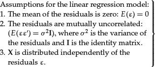
We now make a set of assumptions that are standard in regression analysis and that we will progressively relax. The assumptions for the linear regression model with normally distributed residuals are:

(16)

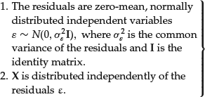
The regression equation can then be written: E(Y|X) = Xβ. The residuals form a sequence of independent variables. They can therefore be regarded as a strict white-noise sequence. As the residuals are independent draws from the same normal distribution, we can compute the log-likelihood function as follows:

(17)

The maximum likelihood (ML) principle requires maximization of the log-likelihood function. Maximizing the log-likelihood function entails first solving the equations:

These equations can be explicitly written as follows:

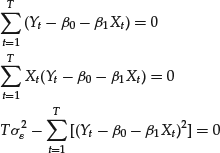
A little algebra shows that solving the first two equations yields

(18)

where

and where are the empirical standard deviations of the sample variables X, Y respectively. Substituting these expressions in the third equation

yields the variance of the residuals:

(19)

In the matrix notation established above, we can write the estimators as follows:

(20)

For the variance of the regression:

(21)

A comment is in order. We started with T pairs of given data (Xi, Yi), i = 1, … , T and then attempted to explain these data as a linear regression Y = β1X + β0 + ε. We estimated the coefficients (β1, β2) with maximum likelihood estimation (MLE) methods. Given this estimate of the regression coefficients, the estimated variance of the residuals is given by equation (22). Note that equation (22) is the empirical variance of residuals computed using the estimated regression parameters. A large variance of the residuals indicates that the level of noise in the process (i.e., the size of the unexplained fluctuations of the process) is high.

Generalization to Multiple Independent Variables

The above discussion of the MLE method generalizes to multiple independent variables, N. We are empirically given a set of T observations that we organize in matrix form,

(22)

and the regression coefficients and error terms in the vectors,

(23)

The matrix X which contains all the regressors is called the design matrix. The regressors X can be deterministic, the important condition being that the residuals are independent. One of the columns can be formed by 1s to allow for a constant term (intercept). Our objective is to explain the data as a linear regression:

We make the same set of assumptions given by equation (17) as we made in the case of a single regressor. Using the above notation, the loglikelihood function will have the form

(24)

The maximum likelihood conditions are written as

(25)

These equations are called normal equations. Solving the system of normal equations gives the same form for the estimators as in the univariate case:

(26)

The variance estimator is not unbiased. It can be demonstrated that to obtain an unbiased estimator we have to apply a correction that takes into account the number of variables by replacing T with T − N, assuming T > N:

(27)

The MLE method requires that we know the functional form of the distribution. If the distribution is known but not normal, we can still apply the MLE method but the estimators will be different. We will not here discuss further MLE for nonnormal distributions.

Ordinary Least Squares Method

We now establish the relationship between the MLE principle and the ordinary least squares (OLS) method. OLS is a general method to approximate a relationship between two or more variables. We use the matrix notation defined above for MLE method; that is, we assume that observations are described by equation (23) while the regression coefficients and the residuals are described by equation (24).

If we use the OLS method, the assumptions of linear regressions can be weakened. In particular, we need not assume that the residuals are normally distributed but only assume that they are uncorrelated and have finite variance. The residuals can therefore be regarded as a white-noise sequence (and not a strict white-noise sequence as in the previous section). We summarize the linear regression assumptions as follows:

(28)

In the general case of a multivariate regression, the OLS method requires minimization of the sum of the squared residuals. Consider the vector of residuals:

The sum of the squared residuals (SSR) = can be written as SSR = ε′ε. As ε = Y − Xβ, we can also write

The OLS method requires that we minimize the SSR. To do so, we equate to zero the first derivatives of the SSR:

This is a system of N equations. Solving this system, we obtain the estimators:

These estimators are the same estimators obtained with the MLE method; they have an optimality property. In fact, the Gauss-Markov theorem states that the above OLS estimators are the best linear unbiased estimators (BLUE). “Best” means that no other linear unbiased estimator has a lower variance. It should be noted explicitly that OLS and MLE are conceptually different methodologies: MLE seeks the optimal parameters of the distribution of the error terms, while OLS seeks to minimize the variance of error terms. The fact that the two estimators coincide was an important discovery.

SAMPLING DISTRIBUTIONS OF REGRESSIONS

Estimated regression parameters depend on the sample. They are random variables whose distribution is to be determined. As we will see in this section, the sampling distributions differ depending on whether the regressors are assumed to be fixed deterministic variables or random variables.

Let’s first assume that the regressors are fixed deterministic variables. Thus only the error terms and the dependent variable change from sample to sample. The are unbiased estimators and therefore holds. It can also be demonstrated that the following expression for the variance of holds

(29)

where an estimate of σ2 is given by (27).

Under the additional assumption that the residuals are normally distributed, it can be demonstrated that the regression coefficients are jointly normally distributed as follows:

(30)

These expressions are important because they allow us to compute confidence intervals for the regression parameters.

Let’s now suppose that the regressors are random variables. Under the assumptions set forth in (29), it can be demonstrated that the variance of the estimators can be written as follows:

(31)

where the terms E[(X′X)−1 ] and V(X′ε) are the empirical expectation of (X′X)–1 and the empirical variance of (X′ε), respectively.

The following terms are used to describe this estimator of the variance: sandwich estimator, robust estimator, and White estimator. The term sandwich estimator is due to the fact that the term V(X′ε) is sandwiched between the terms E[(X’X)−1]. These estimators are robust because they take into account not only the variability of the dependent variables but also that of the independent variables. Consider that if the regressors are a large sample, the sandwich and the classical estimators are close to each other.

DETERMINING THE EXPLANATORY POWER OF A REGRESSION

The above computations to estimate regression parameters were carried out under the assumption that the data were generated by a linear regression function with uncorrelated and normally distributed noise. In general, we do not know if this is indeed the case. Though we can always estimate a linear regression model on any data sample by applying the estimators discussed above, we must now ask the question: When is a linear regression applicable and how can one establish the goodness (i.e., explanatory power) of a linear regression?

Quite obviously, a linear regression model is applicable if the relationship between the variables is approximately linear. How can we check if this is indeed the case? What happens if we fit a linear model to variables that have nonlinear relationships, or if distributions are not normal? A number of tests have been devised to help answer these questions.

Intuitively, a measure of the quality of approximation offered by a linear regression is given by the variance of the residuals. Squared residuals are used because a property of the estimated relationship is that the sum of the residuals is zero. If residuals are large, the regression model has little explanatory power. However, the size of the average residual in itself is meaningless as it has to be compared with the range of the variables. For example, if we regress stock prices over a broad-based stock index, other things being equal, the residuals will be numerically different if the price is in the range of dollars or in the range of hundreds of dollars.

Coefficient of Determination

A widely used measure of the quality and usefulness of a regression model is given by the coefficient of determination denoted by R2 or R-squared. The idea behind R2 is the following. The dependent variable Y has a total variation given by the following expression:

(32)

where

This total variation is the sum of the variation of the variable Y due to the variation of the regressors plus the variation of residuals . We can therefore define the coefficient of determination:

(33)

as the portion of the total fluctuation of the dependent variable, Y, explained by the regression relation. R2 is a number between 0 and 1: R2 = 0 means that the regression has no explanatory power, R2 = 1 means that the regression has perfect explanatory power. The quantity R2 is computed by software packages that perform linear regressions.

It can be demonstrated that the coefficient of determination R2 is distributed as the well-known Student F distribution. This fact allows one to determine intervals of confidence around a measure of the significance of a regression.

Adjusted R2

The quantity R2 as a measure of the usefulness of a regression model suffers from the problem that a regression might fit data very well in-sample but have no explanatory power out-of-sample. This occurs if the number of regressors is too high. Therefore an adjusted R2 is sometimes used. The adjusted R2 is defined as R2 corrected by a penalty function that takes into account the number p of regressors in the model:

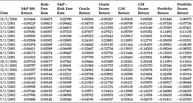
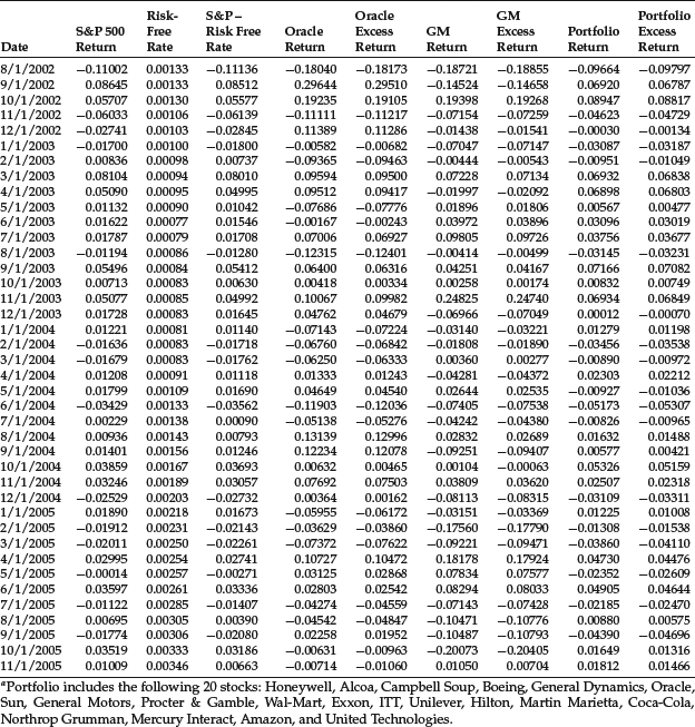
Table 1 Return and Excess Return Data for S&P 500, Oracle, GM, and Portfolioa: 12/1/2000–11/1/2005

(34)

Relation of R2 to Correlation Coefficient

The R2 is the squared correlation coefficient. The correlation coefficient is a number between −1 and +1 that measures the strength of the dependence between two variables. If a linear relationship is assumed, the correlation coefficient has the usual product-moment expression:

(35)

USING REGRESSION ANALYSIS IN FINANCE

This section provides several illustrations of regression analysis in finance as well as the data for each illustration. However, in order to present the data, we limit our sample size.

Characteristic Line for Common Stocks

The characteristic line of a security is the regression of the excess returns of that security on the market excess returns:

where

ri = the security excess return of a security over the risk-free rate
rM = the market excess return of the market over the risk-free rate

We computed the characteristic lines of two common stocks, Oracle and General Motors (GM), and a randomly created portfolio consisting of 20 stocks equally weighted. We used the S&P 500 Index as a proxy for the market returns and the 90-day Treasury rate as a proxy for the risk-free rate. The return and excess return data are shown in Table 1. Note that there are 60 monthly observations used to estimate the characteristic line from December 2000 to November 2005. The 20 stocks comprising the portfolio are shown at the bottom of Table 1.

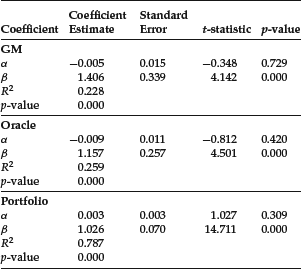
The estimated parameters for the two stocks and the portfolios are reported in Table 2. As can be seen from the table, the intercept term is not statistically significant; however, the slope, referred to as the beta of the characteristic line, is statistically significant. Typically for individual stocks, the R2 ranges from 0.15 to 0.65. For Oracle and GM the R2 is 0.23 and 0.26, respectively. In contrast, for a randomly created portfolio, the R2 is considerably higher. For our 20-stock portfolio, the R2 is 0.79.

Note that some researchers estimate a stock’s beta by using returns rather than excess returns. The regression estimated is referred to as the single-index market model. This model was first suggested by Markowitz as a proxy measure of the covariance of a stock with an index so that the full mean-variance analysis need not be performed. While the approach was mentioned by Markowitz (1959) in a footnote in his book, it was Sharpe (1963) who investigated this further. It turns out that the beta estimated using both the characteristic line and the single-index market model do not differ materially. For example, for our 20-stock portfolio, the betas differed only because of rounding off.

Empirical Duration of Common Stock

A commonly used measure of the interest-rate sensitivity of an asset’s value is its duration. Duration is interpreted as the approximate percentage change in the value of an asset for a 100-basis-point change in interest. Duration can be estimated by using a valuation model or empirically by estimating from historical returns the sensitivity of the asset’s value to changes in interest rates. When duration is measured in the latter way, it is called empirical duration. Since it is estimated using regression analysis, it is sometimes referred to as regression-based duration.

Table 2 Characteristic Line of the Common Stock of General Motors, Oracle, and Portfolio: 12/1/2000–11/1/2005

A simple linear regression for computing empirical duration using monthly historical data (see Reilly, Wright, and Johnson, 2007) is

where

yit = the percentage change in the value of asset i for month t
xt = the change in the Treasury yield for month t

The estimated βi is the empirical duration for asset i.

We will apply this linear regression to monthly data from October 1989 to October 2003 shown in Table 31 for the following asset indexes:

• Electric Utility sector of the S&P 500
• Commercial Bank sector of the S&P 500
• Lehman U.S. Aggregate Bond Index (now the Barclays Capital U.S. Aggregate Bond Index)

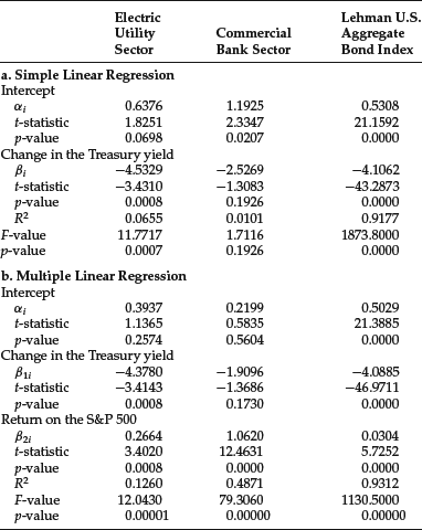
The yield change (xt) is measured by the Lehman Treasury Index. The regression results are shown in Table 4. We report the empirical duration (βi), the t-statistic, the p-value, the R2, and the intercept term. Negative values are reported for the empirical duration. In practice, however, the duration is quoted as a positive value. For the Electric Utility sector and the Lehman U.S. Aggregate Bond Index, the empirical duration is statistically significant at any reasonable level of significance.

Table 3 Data for Empirical Duration Illustration

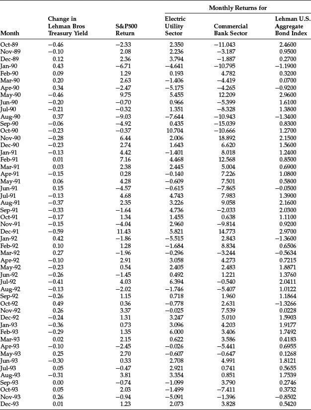
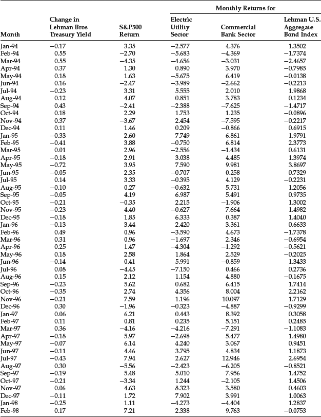
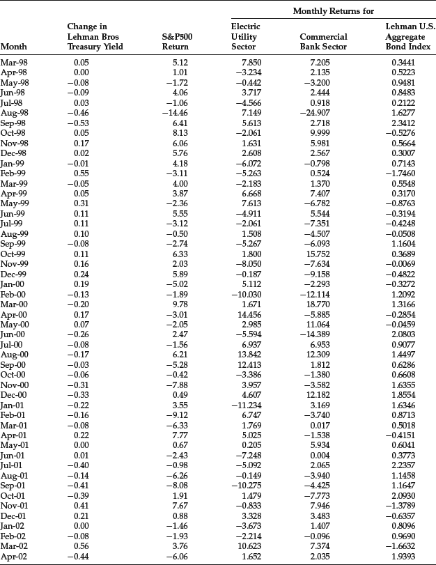
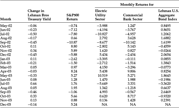
Table 4 Estimation of Regression Parameters for Empirical Duration

A multiple regression model to estimate the empirical duration that has been suggested is

where yit and x1t are the same as for the simple linear regression and x2t is the return on the S&P 500. The results for this model are also shown in Table 4.

The results of the multiple regression indicate that the returns for the Electric Utility sector are affected by both the change in Treasury rates and the return on the stock market as proxied by the S&P 500. For the Commercial Bank sector, the coefficient of the changes in Treasury rates is not statistically significant, however the coefficient of the return on the S&P 500 is statistically significant. The opposite is the case for the Lehman U.S. Aggregate Bond Index. It is interesting to note that the duration for the Lehman U.S. Aggregate Bond Index as reported by Lehman Brothers was about 4.55 in November 2003. The empirical duration is 4.1. While the sign of the coefficient that is an estimate of duration is negative (which means the price moves in the opposite direction to the change in interest rates), mar ket participants talk in terms of the positive value of duration for a bond that has this characteristic.

Predicting the 10-Year Treasury Yield2

The U.S. Department of the Treasury issues two types of securities: zero-coupon securities and coupon securities. Securities issued with one year or less to maturity are called Treasury bills; they are issued as zero-coupon instruments. Treasury securities with more than one year to maturity are issued as coupon-bearing securities. Treasury securities from more than one year up to 10 years of maturity are called Treasury notes; Treasury securities with a maturity in excess of 10 years are called Treasury bonds. The U.S. Treasury auctions securities of specified maturities on a regular calendar basis. The Treasury currently issues 30-year Treasury bonds but had stopped issuance of them from October 2001 to January 2006.

An important Treasury coupon bond is the 10-year Treasury note. In this illustration we will try to forecast this rate based on two independent variables suggested by economic theory. A well-known theory of interest rates is that the interest rate in any economy consists of two components. This relationship is known as Fisher’s law. The first is the expected rate of inflation. The second is the real rate of interest. We use regression analysis to produce a model to forecast the yield on the 10-year Treasury note (simply, the 10-year Treasury yield)—the dependent variable—and the expected rate of inflation (simply, expected inflation) and the real rate of interest (simply, real rate).

The 10-year Treasury yield is observable, but we need a proxy for the two independent variables (i.e., the expected rate of inflation and the real rate of interest at the time) as they are not observable at the time of the forecast. Keep in mind that since we are forecasting, we do not use as our independent variable information that is unavailable at the time of the forecast. Consequently, we need a proxy available at the time of the forecast.

The inflation rate is available from the U.S. Department of Commerce. However, we need a proxy for expected inflation. We can use some type of average of past inflation as a proxy. In our model, we use a 5-year moving average. There are more sophisticated methodologies for calculating expected inflation, but the 5-year moving average is sufficient for our illustration. For example, one can use an exponential smoothing of actual inflation, a methodology used by the OECD. For the real rate, we use the rate on 3-month certificates of deposit (CDs). Again, we use a 5-year moving average.

The monthly data for the three variables from November 1965 to December 2005 (482 observations) are provided in Table 5. The regression results are reported in Table 6. As can be seen, the coefficients of both independent variables are positive (as would be predicted by economic theory) and highly significant.

Table 5 Monthly Data for 10-Year Treasury Yield, Expected Inflation, and Real Rate: November 1965–December 2005

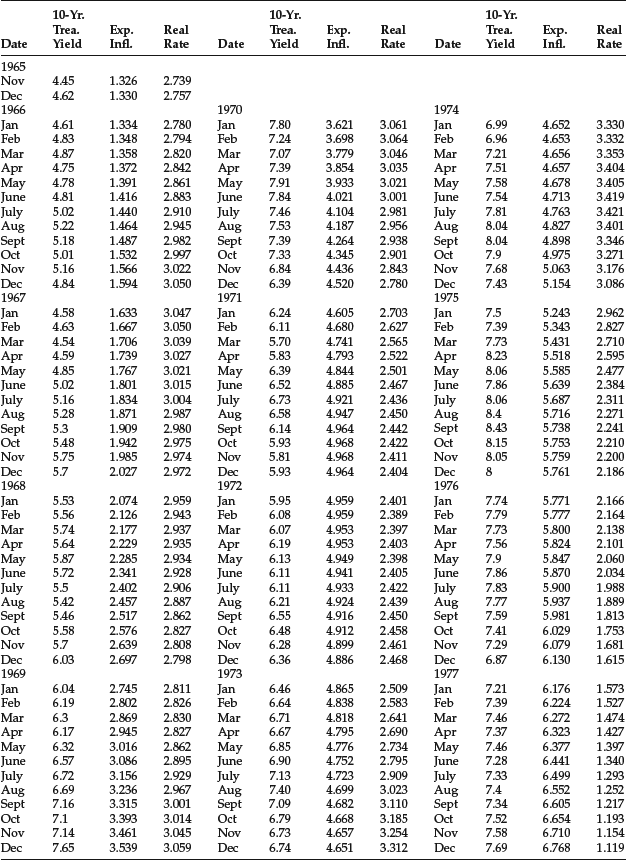
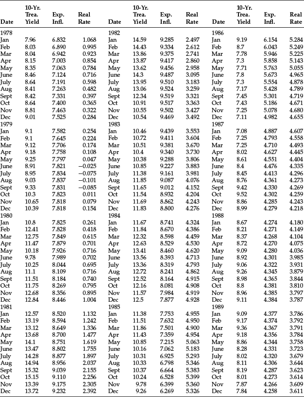
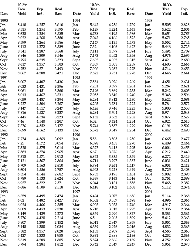
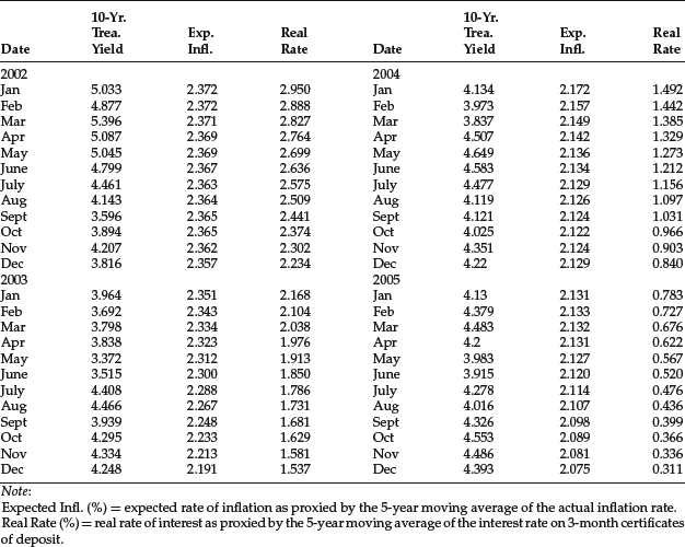
Table 6 Results of Regression for Forecasting 10-Year Treasury Yield

NONNORMALITY AND AUTOCORRELATION OF THE RESIDUALS

In the above discussion we assumed that there is no correlation between the residual terms. Let’s now relax these assumptions. The correlation of the residuals is critical from the point of view of estimation. Autocorrelation of residuals is quite common in financial estimation where we regress quantities that are time series.

A time series is said to be autocorrelated if each term is correlated with its predecessor so that the variance of each term is partially explained by regressing each term on its predecessor.

Recall from the previous section that we organized regressor data in a matrix called the design matrix. Suppose that both regressors and the variable Y are time series data, that is, every row of the design matrix corresponds to a moment in time. The regression equation is written as follows:

Suppose that residuals are correlated. This means that in general E[εiεj] = σij ≠ 0. Thus the variance-covariance matrix of the residuals {σij} will not be a diagonal matrix as in the case of uncorrelated residuals, but will exhibit nonzero off-diagonal terms. We assume that we can write

where Ω is a positive definite symmetric matrix and σ is a parameter to be estimated.

If residuals are correlated, the regression parameters can still be estimated without biases using the formula given by (26). However, this estimate will not be optimal in the sense that there are other estimators with lower variance of the sampling distribution. An optimal linear unbiased estimator has been derived. It is called Aitken’s generalized least squares (GLS) estimator and is given by

(36)

where is the residual correlation matrix.

The GLS estimators vary with the sampling distribution. It can also be demonstrated that the variance of the GLS estimator is also given by the following “sandwich” formula:

(37)

This expression is similar to equation (28) with the exception of the sandwiched term . Unfortunately, (37) cannot be estimated without first knowing the regression coefficients. For this reason, in the presence of correlation of residuals, it is common practice to replace static regression models with models that explicitly capture autocorrelations and produce uncorrelated residuals.

The key idea here is that autocorrelated residuals signal that the modeling exercise has not been completed. If residuals are autocorrelated, this signifies that the residuals at a generic time t can be predicted from residuals at an earlier time. For example, suppose that we are linearly regressing a time series of returns rt on N factors:

Suppose that the residual terms εt are autocorrelated and that we can write regressions of the type

where ηt are now uncorrelated variables. If we ignore this autocorrelation, valuable forecasting information is lost. Our initial model has to be replaced with the following model:

with the initial conditions ε0.

Detecting Autocorrelation

How do we detect the autocorrelation of residuals? Suppose that we believe that there is a reasonable linear relationship between two variables, for instance stock returns and some fundamental variable. We then perform a linear regression between the two variables and estimate regression parameters using the OLS method. After estimating the regression parameters, we can compute the sequence of residuals. At this point, we can apply tests such as the Durbin-Watson test or the Dickey-Fuller test to gauge the autocorrelation of residuals. If residuals are auto-correlated, we should modify the model.

PITFALLS OF REGRESSIONS

It is important to understand when regressions are correctly applicable and when they are not. In addition to the autocorrelation of residuals, there are other situations where it would be inappropriate to use regressions. In particular, we analyze the following cases, which represent possible pitfalls of regressions:

• Spurious regressions with integrated variables
• Collinearity
• Increasing the number of regressors

Spurious Regressions

The phenomenon of spurious regressions, observed by Yule in 1927, led to the study of cointegration. We encounter spurious regressions when we perform an apparently meaningful regression between variables that are independent. A typical case is a regression between two independent random walks. Regressing two independent random walks, one might find very high values of R2 even if the two processes are independent. More in general, one might find high values of R2 in the regression of two or more integrated variables, even if residuals are highly correlated.

Testing for regressions implies testing for cointegration. Anticipating what will be discussed there, it is always meaningful to perform regressions between stationary variables. When variables are integrated, regressions are possible only if variables are cointegrated. This means that residuals are a stationary (though possibly autocorrelated) process. As a rule of thumb, Granger and Newbold (1974) observe that if the R2 is greater than the Durbin-Watson statistics, it is appropriate to investigate if correlations are spurious.

Collinearity

Collinearity, also referred to as multicollinearity, occurs when two or more regressors have a linear deterministic relationship. For example, there is collinearity if the design matrix

exhibits two or more columns that are perfectly proportional. Collinearity is essentially a numerical problem. Intuitively, it is clear that it creates indeterminacy as we are regressing twice on the same variable. In particular, the standard estimators given by (26) and (27) cannot be used because the relative formulas become meaningless.

In principle, collinearity can be easily resolved by eliminating one or more regressors. The problem with collinearity is that some variables might be very close to collinearity, thus leading to numerical problems and indeterminacy of results. In practice, this might happen for many different numerical artifacts. Detecting and analyzing collinearity is a rather delicate problem. In principle one could detect collinearity by computing the determinant of X’X. The difficulty resides in analyzing situations where this determinant is very small but not zero. One possible strategy for detecting and removing collinearity is to go through a process of orthogonalization of variables. (See Hendry [1995].)

Increasing the Number of Regressors

Increasing the number of regressors does not always improve regressions. The econometric theorem known as Pyrrho’s lemma relates to the number of regressors. (See Dijkstra [1995].) Pyrrho’s lemma states that by adding one special regressor to a linear regression, it is possible to arbitrarily change the size and sign of regression coefficients as well as to obtain an arbitrary goodness of fit. This result, rather technical, seems artificial as the regressor is an artificially constructed variable. It is, however, a perfectly rigorous result; it tells us that, if we add regressors without a proper design and testing methodology, we risk obtaining spurious results.

Pyrrho’s lemma is the proof that modeling results can be arbitrarily manipulated in-sample even in the simple context of linear regressions. In fact, by adding regressors one might obtain an excellent fit in-sample though these regressors might have no predictive power out-of-sample. In addition, the size and even the sign of the regression relationships can be artificially altered in-sample.

The above observations are especially important for those financial models that seek to forecast prices, returns, or rates based on regressions over economic or fundamental variables. With modern computers, by trial and error, one might find a complex structure of regressions that give very good results in-sample but have no real forecasting power.

KEY POINTS

• In regression analysis, the relationship between a random variable, called the dependent variable, and one or more variables referred to as the independent variables, regressors, or explanatory variables (which can be random variables or deterministic variables) is estimated.
• Factorization, which involves expressing a joint density as a product of a marginal density and a conditional density, is the conceptual basis of financial econometrics.
• An econometric model is a probe that extracts independent samples—the noise terms—from highly dependent variables.
• Regressions have a twofold nature: they can be either (1) the representation of dependence in terms of conditional expectations and conditional distributions or (2) the representation of dependence of random variables on deterministic parameters.
• In many applications in financial modeling, the regressors are deterministic variables. Therefore, on a conceptual level, regressions with deterministic regressors are different from cases where regressors are random variables. In particular, a financial modeler cannot view the regression as a conditional expectation.
• There are two main estimation techniques for estimating the parameters of a regression: maximum likelihood method and ordinary least squares method. The maximum likelihood principle requires maximization of the log-likelihood function. The ordinary least squares method requires minimization of the sum of the squared residuals. The ordinary least squares estimators are the best linear unbiased estimators.
• Because the estimated regression parameters depend on the sample, they are random variables whose distribution is to be determined. The sampling distributions differ depending on whether the regressors are assumed to be fixed deterministic variables or random variables.
• A measure of the quality of approximation offered by a linear regression is given by the variance of the residuals. If residuals are large, the regression model has little explanatory power. However, the size of the average residual in itself is meaningless as it has to be compared with the range of the variables. A widely used measure of the quality and usefulness of a regression model is given by the coefficient of determination, denoted by R2 or R-squared, that can attain a value from zero to one. The adjusted R2 is defined as R2 corrected by a penalty function that takes into account the number of regressors in the model.
• Stepwise regression is a model-building technique for regression designs. The two methodologies for stepwise regression are the backward stepwise method and the backward removal method.
• A time series is said to be autocorrelated if each term is correlated with its predecessor so that the variance of each term is partially explained by regressing each term on its predecessor. Autocorrelation of residuals, a violation of the regression model assumptions, is quite common in financial estimation where financial modelers regress quantities that are time series. When there is autocorrelation present in a time series, the generalized least squares estimation method is used. The Durbin-Watson test or the Dickey-Fuller test can be utilized to gauge test for the presence of autocorrelation for the residuals.
• Three other situations where there are possible pitfalls of using regressions are spurious regressions with integrated variables, collinearity, and increasing the number of regressors. Spurious regressions occur when an apparently meaningful regression between variables that are independent is estimated. Collinearity occurs when two or more regressors in a regression model have a linear deterministic relationship.
• Pyrrho’s lemma, which relates to the number of regressors in a regression model, states that by adding one special regressor to a linear regression, it is possible to arbitrarily change the size and sign of regression coefficients as well as to obtain an arbitrary goodness of fit. Pyrrho’s lemma is the proof that modeling results can be arbitrarily manipulated in-sample even in the simple context of linear regressions.

NOTES

1. The data were supplied by David Wright of Northern Illinois University.

2. We are grateful to Robert Scott of the Bank for International Settlement for suggesting this illustration and for providing the data.

REFERENCES

Bradley, B., and Taqqu, M. (2003). Financial risk and heavy tails. In S. T. Rachev (ed.), Handbook of Heavy Tailed Distributions in Finance (pp. 35–103). Amsterdam: Elsevier/North Holland.

Dijkstra, T. K. (1995). Pyrrho’s lemma, or have it your way. Metrica 42: 119–225.

Embrechts, P., McNeil, A., and Straumann, D. (2002). Correlation and dependence in risk management: Properties and pitfalls. In M. Dempster (ed.), Risk Management: Value at Risk and Beyond (pp. 176–223). Cambridge: Cambridge University Press.

Granger, C., and Newbold, P. (1974). Spurious regression in econometrics. Journal of Econometrics 2: 111–120.

Hendry, D. F. (1995). Dynamic Econometrics. Oxford: Oxford University Press.

Markowitz, H. M. (1959). Portfolio Selection: Efficient Diversification of Investments. New Haven, CT: Cowles Foundation for Research in Economics.

Reilly, F. K., Wright, D. J., and Johnson, R. R. (2007). An analysis of the interest rate sensitivity of common stocks. Journal of Portfolio Management 33, 2: 85–107.

Sharpe, W. F. (1963). A simplified model for portfolio analysis. Management Science 9, 1: 277–293.