Categorical and Dummy Variables in Regression Models
There are many times in the application of regression analysis when the financial modeler will need to include a categorical variable rather than a continuous variable as a regressor. Categorical variables are variables that represent group membership. For example, given a set of bonds, the rating is a categorical variable that indicates to what category—AA, BB, and so on—each bond belongs. A categorical variable does not have a numerical value or a numerical interpretation in itself. Thus the fact that a bond is in category AA or BB does not, in itself, measure any quantitative characteristic of the bond, though quantitative attributes such as a bond’s yield spread can be associated with each category.
In this entry, we will discuss how to deal with regressors that are categorical variables in a regression model. There are also applications where the dependent variable may be a categorical variable. For example, the dependent variable could be bankruptcy or nonbankruptcy of a company over some period of time. In such cases, the product of a regression is a probability. Probability models of this type include linear probability, logit regression, and probit linear models.
INDEPENDENT CATEGORICAL VARIABLES
Categorical input variables are used to cluster input data into different groups. That is, suppose we are given a set of input-output data and a partition of the data set in a number of subsets Ai so that each data point belongs to one and only one set. The Ai represent a categorical input variable. In financial econometrics categories might represent, for example, different market regimes, economic states, ratings, countries, industries, or sectors.
We cannot, per se, mix quantitative input variables and categorical variables. For example, we cannot sum yield spreads and their ratings. However, we can perform a transformation that allows the mixing of categorical and quantitative variables. Let’s see how. Suppose first that there is only one categorical input variable D, one quantitative input variable X, and one quantitative output variable Y Consider our set of quantitative data, that is, quantitative observations. We organize data in a matrix form as usual:

Suppose data belong to two categories. An explanatory variable that distinguishes only two categories is called a dichotomous variable. The key is to represent a dichotomous categorical variable as a numerical variable D, called a dummy variable, that can assume the two values 0,1. We can now add the variable D to the input variables to represent membership in one or the other group:

If Di = 0, the data Xi belong to the first category; if Di = 1, the data Xi belong to the second category.
Consider now the regression equation
![]()
In financial econometric applications, the index i will be time or a variable that identifies a cross section of assets, such as bond issues. Consider that we can write three separate regression equations, one for those data that correspond to D = 1, one for those data that correspond to D = 0, and one for the fully pooled data. Suppose now that the three equations differ by the intercept term but have the same slope. Let’s explicitly write the two equations for those data that correspond to D = 1 and for those data that correspond to D = 0:
![]()
where i defines the observations that belong to the first category when the dummy variable D assumes value 0 and also defines the observations that belong to the second category when the dummy variable D assumes value 1. If the two categories are recession and expansion, the first equation might hold in periods of expansion and the second in periods of recession. If the two categories are investment-grade bonds and noninvestment-grade bonds, the two equations apply to different cross sections of bonds, as will be illustrated in an example later in this entry.
Observe now that, under the assumption that only the intercept term differs in the two equations, the two equations can be combined into a single equation in the following way:
![]()
where γ = β01 − β00 represents the difference of the intercept for the two categories. In this way we have defined a single regression equation with two independent quantitative variables, X, D, to which we can apply all the usual tools of regression analysis, including the ordinary least squares (OLS) estimation method and all the tests. By estimating the coefficients of this regression, we obtain the common slope and two intercepts. Observe that we would obtain the same result if the categories were inverted. However, the interpretation of the estimated parameter for the categorical variable would differ depending on which category is omitted.
Thus far we have assumed that there is no interaction between the categorical and the quantitative variable, that is, the slope of the regression is the same for the two categories. This means that the effects of variables are additive; that is, the effect of one variable is added regardless of the value taken by the other variable. In many applications, this is an unrealistic assumption.
Using dummy variables, the treatment is the same as that applied to intercepts. Consider the regression equation Yi = β0 + β1Xi + εi and write two regression equations for the two categories as we did above:
![]()
We can couple these two equations in a single equation as follows:
![]()
where δ = β11 − β10. In fact, the above equation is identical to the first equation for Di = 0 and to the second for Di = 1. This regression can be estimated with the usual LS methods.
In practice, it is rarely appropriate to consider only interactions and not the intercept, which is the main effect. We call marginalization the fact that the interaction effect is marginal with respect to the main effect. However, we can easily construct a model that combines both effects. In fact we can write the following regression adding two variables, the dummy D and the interaction DX:
![]()
This regression equation, which now includes three regressors, combines both effects.
The above process of introducing dummy variables can be generalized to regressions with multiple variables. Consider the following regression:
![]()
where data can be partitioned in two categories with the use of a dummy variable:

We can introduce the dummy D as well as its interaction with the N quantitative variable and thus write the following equation:
![]()
The above discussion depends critically on the fact that there are only two categories, a fact that allows one to use the numerical variable 0,1 to identify the two categories. However, the process can be easily extended to multiple categories by adding dummy variables. Suppose there are K > 2 categories. An explanatory variable that distinguishes between more than two categories is called a polytomous variable.
Suppose there are three categories, A, B, and C. Consider a dummy variable D1 that assumes a value one on the elements of A and zero on all the others. Let’s now add a second dummy variable D2 that assumes the value one on the elements of the category B and zero on all the others. The three categories are now completely identified: A is identified by the values 1,0 of the two dummy variables, B by the values 0,1, and C by the values 0,0. Note that the values 1,1 do not identify any category. This process can be extended to any number of categories. If there are K categories, we need K − 1 dummy variables.
How can we determine if a given categorization is useful? It is quite obvious that many categorizations will be totally useless for the purpose of any econometric regression. If we categorize bonds in function of the color of the logo of the issuer, it is quite obvious that we obtain meaningless results. In other cases, however, distinctions can be subtle and important. Consider the question of market regime shifts or structural breaks. These are delicate questions that can be addressed only with appropriate statistical tests.
A word of caution about statistical tests is in order. Statistical tests typically work under the assumptions of the model and might be misleading if these assumptions are violated. If we try to fit a linear model to a process that is inherently nonlinear, tests might be misleading. It is good practice to use several tests and to be particularly attentive to inconsistencies between test results. Inconsistencies signal potential problems in applying tests, typically model misspecification.
The t-statistic applied to the regression coefficients of dummy variables offer a set of important tests to judge which regressors are significant. The t-statistics are the coefficients divided by their respective squared errors. The p-value associated with each coefficient estimate is the probability of the hypothesis that the corresponding coefficient is zero, that is, that the corresponding variable is irrelevant.
We can also use the F-test to test the significance of each specific dummy variable. To do so we can run the regression with and without that variable and form the corresponding F-test. The Chow test is the F-test to gauge if all the dummy variables are collectively irrelevant (see Chow, 1960). The Chow test is an F-test of mutual exclusion, written as follows:
![]()
where
SSR1 = the squared sum of residuals of the regression run with data in the first category without dummy variables
SSR2 = the squared sum of residuals of the regression run with data in the second category without dummy variables
SSR = the squared sum of residuals of the regression run with fully pooled data without dummy variables
Observe that SSR1 + SSR2 is equal to the squared sum of residuals of the regression run on fully pooled data but with dummy variables. Thus the Chow test is the F-test of the unrestricted regressions with and without dummy variables.
Illustration: Predicting Corporate Bond Yield Spreads
To illustrate the use of dummy variables, we will estimate a model to predict corporate bond spreads.1 The regression is relative to a cross section of bonds. The regression equation is the following:
![]()
where
Spreadi = option-adjusted spread (in basis points) for the bond issue of company i
Couponi = coupon rate for the bond of company i, expressed without considering percentage sign (i.e., 7.5% = 7.5)
CoverageRatioi = earnings before interest, taxes, depreciation and amortization (EBITDA) divided by interest expense for company i
LoggedEBITi = logarithm of earnings (earnings before interest and taxes, EBIT, in millions of dollars) for company i
The dependent variable, Spread, is not measured by the typically nominal spread but by the option-adjusted spread. This spread measure adjusts for any embedded options in a bond (see Chapter 6 in Fabozzi, 2006).
Theory would suggest the following properties for the estimated coefficients:
- The higher the coupon rate, the greater the issuer’s default risk and hence the larger the spread. Therefore, a positive coefficient for the coupon rate is expected.
- A coverage ratio is a measure of a company’s ability to satisfy fixed obligations, such as interest, principal repayment, or lease payments. There are various coverage ratios. The one used in this illustration is the ratio of the earnings before interest, taxes, depreciation, and amortization (EBITDA) divided by interest expense. Since the higher the coverage ratio the lower the default risk, an inverse relationship is expected between the spread and the coverage ratio; that is, the estimated coefficient for the coverage ratio is expected to be negative.
- There are various measures of earnings reported in financial statements. Earnings in this illustration is defined as the trailing 12-months earnings before interest and taxes (EBIT). Holding other factors constant, it is expected that the larger the EBIT, the lower the default risk and therefore an inverse relationship (negative coefficient) is expected.
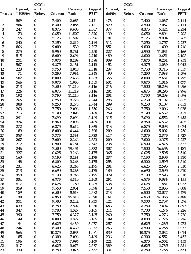
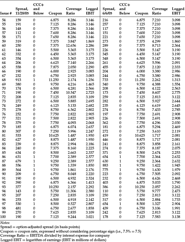
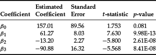
We used 100 observations at two different dates, 6/6/05 and 11/28/05; thus there are 200 observations in total. This will allow us to test if there is a difference in the spread regression for investment-grade and noninvestment grade bonds using all observations. We will then test to see if there is any structural break between the two dates. We organize the data in matrix form as usual. Data are shown in Table 1. The second column indicates that data belong to two categories and suggests the use of one dummy variable. Another dummy variable is used later to distinguish between the two dates. Let’s first estimate the regression equation for the fully pooled data, that is, all data without any distinction in categories. The estimated coefficients for the model and their corresponding t-statistics are shown below:
Table 1 Regression Data for the Bond Spread Application: 11/28/2005 and 06/06/2005
Other regression results are:

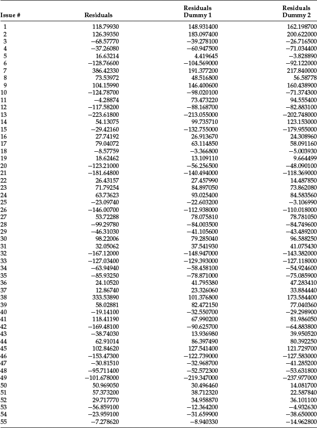
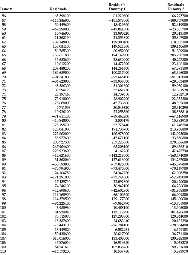
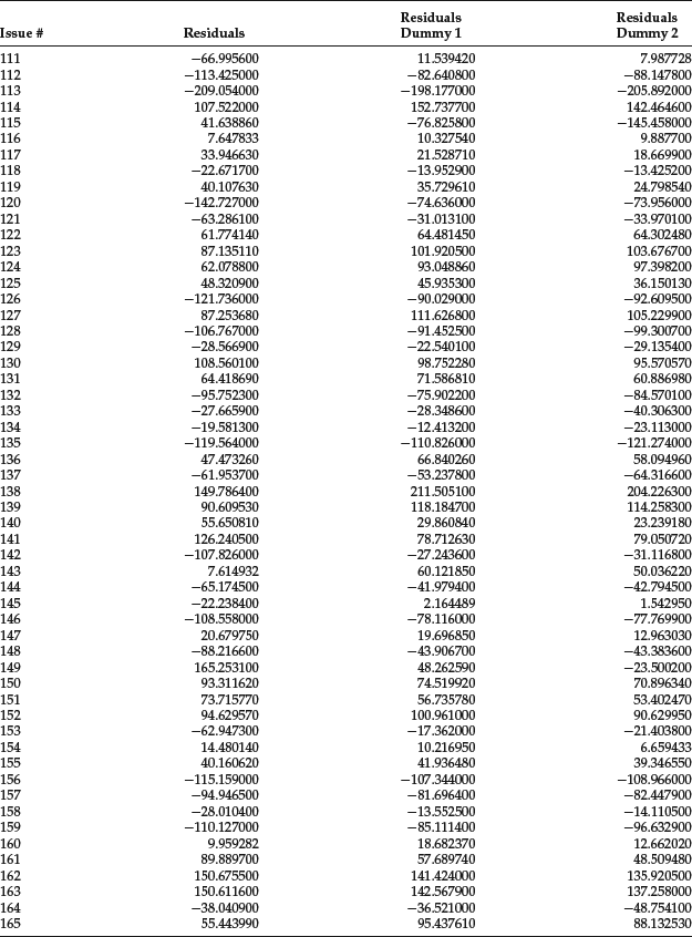
Given the high value of the F-statistic and the p-value close to zero, the regression is significant. The coefficient for the three regressors is statistically significant and has the expected sign. However, the intercept term is not statistically significant. The residuals are given in the first column of Table 2.
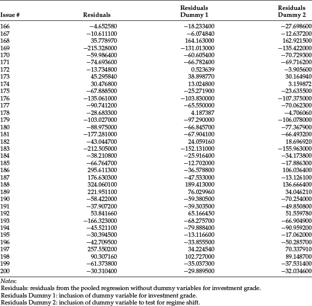
Table 2 Illustration of Residuals and Leverage for Corporate Bond Spread
Let’s now analyze if we obtain a better fit if we consider the two categories of investment-grade and below investment-grade bonds. It should be emphasized that this is only an exercise to show the application of regression analysis. The conclusions we reach are not meaningful from an econometric point of view given the small size of the database. The new equation is written as follows:

There are now seven variables and eight parameters to estimate. The estimated model coefficients and the t-statistics are shown below:
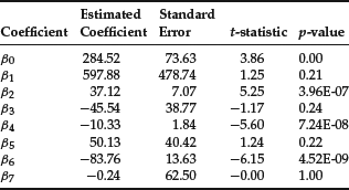
Other regression results are:

The Chow test has the value 16.60. The F-statistic and the Chow test suggest that the use of dummy variables has greatly improved the goodness of fit of the regression, even after compensating for the increase in the number of parameters. The residuals of the model without and with dummy variable D1 are shown, respectively, in the second and third columns of Table 2.
Now let’s use dummy variables to test if there is a regime shift between the two dates. This is a common use for dummy variables in practice. To this end we create a new dummy variable that has the value 0 for the first date 11/28/05 and 1 for the second date 6/6/05. The new equation is written as follows:

as in the previous case but with a different dummy variable. There are seven independent variables and eight parameters to estimate. The estimated model coefficients and t-statistics are shown below:
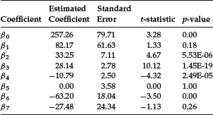
Other regression statistics are:

The Chow test has the value 14.73. The F-statistics and the Chow test suggest that there is indeed a regime shift and that the spread regressions at the two different dates are different. Again, the use of dummy variables has greatly improved the goodness of fit of the regression, even after compensating for the increase in the number of parameters. The residuals of the model with dummy variables D2 are shown in the next-to-the-last column of Table 2.
Illustration: Testing the Mutual Fund Characteristic Lines in Different Market Environments
The characteristic line of a mutual fund is the regression of the excess returns of a mutual fund on the market’s excess returns:
![]()
where
yit = mutual fund i’s excess return over the risk-free rate
xt = market excess return over the risk-free rate
αi and βi = the regression parameters to be estimated for mutual fund i
We will first estimate the characteristic line for two large-cap mutual funds. Since we would prefer not to disclose the name of each fund, we simply refer to them as A and B. (Neither mutual fund selected is an index fund.) Because the two mutual funds are large-cap funds, the S&P 500 was used as the benchmark. The risk-free rate used was the 90-day Treasury bill rate. Ten years of monthly data were used from January 1, 1995 to December 31, 2004. The data are reported in Table 3. The first column in the table shows the month. The second and third columns give the return on the market return (rMt) and risk-free rate (rft), respectively. The fifth column is the excess market return, which is xt in the regression equation. The seventh and eighth columns show the returns for mutual funds A and B, respectively. The excess returns for the two mutual funds (yit) are given in the last two columns. The other columns will be explained shortly.
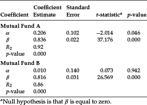
The results of the above regression for both mutual funds are shown in Table 4. The estimated β for both mutual funds is statistically significantly different from zero.
Let’s now perform a simple application of the use of dummy variables by determining if the slope (beta) of the two mutual funds is different in a rising stock market (“up market”) and a declining stock market (“down market”). To test this, we can write the following multiple regression model:
![]()
where Dt is the dummy variable that can take on a value of 1 or 0. We will let
![]()
The coefficient for the dummy variable is β2i. If that coefficient is statistically significant, then for the mutual fund:
Table 3 Data for Estimating Mutual Fund Characteristic Line with a Dummy Variable
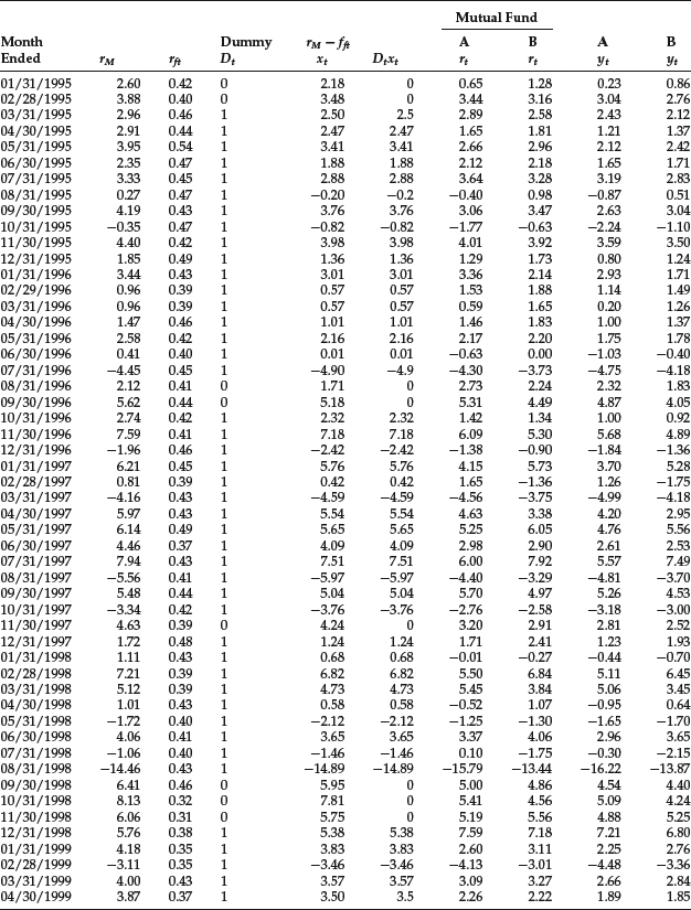
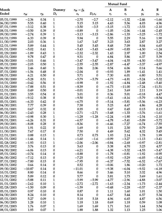
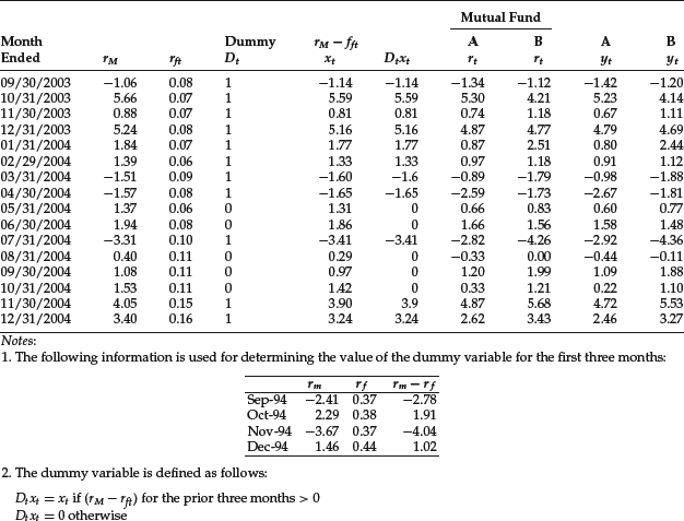
Table 4 Characteristic Line for Mutual Funds A and B
![]()
If β2i is not statistically significant, then there is no difference in βi for up and down markets.
In our illustration, we have to define what we mean by an up and a down market. We will define an up market precisely as one where the average excess return (market return over the risk-free rate or (rMt − rft)) for the prior three months is greater than zero. Then

The regressor will then be

The data are presented in Table 3. The fourth column provides the coding for the dummy variable, Dt, and the sixth column shows the product of Dt and xt.The regression results for the two mutual funds are shown in Table 5. The adjusted R2 is 0.93 and 0.83 for mutual funds A and B, respectively.
Table 5 Regression Results for Dummy Variable Regression for Mutual Funds A and B
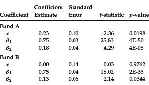
For both funds, β2i is statistically significantly different from zero. Hence, for these two mutual funds, there is a difference in the βi for up and down markets. From the results reported previously, we would find that:
| Mutual Fund A | Mutual Fund B | |
| Down market βi (= β1i) | 0.75 | 0.75 |
| Up market βi (= β1i + β2i) | 0.93 (= 0.75 + 0.18) | 0.88 (= 0.75 + 0.13) |
DEPENDENT CATEGORICAL VARIABLES
Thus far we have discussed models where the independent variables can be either quantitative or categorical while the dependent variable is quantitative. Let’s now discuss models where the dependent variable is categorical. Recall that a regression model can be interpreted as a conditional probability distribution. Suppose that the dependent variable is a categorical variable Y that can assume two values, which we represent conventionally as 0 and 1. The probability distribution of the dependent variable is then a discrete function:
![]()
A regression model where the dependent variable is a categorical variable is therefore a probability model; that is, it is a model of the probability p given the values of the independent variables X:
![]()
In the following sections we will discuss three probability models: the linear probability model, the probit regression model, and the logit regression model.
Linear Probability Model
The linear probability model assumes that the function f(X) is linear. For example, a linear probability model of default assumes that there is a linear relationship between the probability of default and the factors that determine default.
![]()
The parameters of the model can be obtained by using ordinary least squares applying the estimation methods of multiple regression models entry. Once the parameters of the model are estimated, the predicted value for P(Y) can be interpreted as the event probability such as the probability of default in our previous example. Note, however, that when using a linear probability model, in this entry the R2 is used only if all the independent variables are also binary variables.
A major drawback of the linear probability model is that the predicted value may be negative. In the probit regression and logit regression models described below, the predicted probability is forced to be between 0 and 1.
Probit Regression Model
The probit regression model is a nonlinear regression model where the dependent variable is a binary variable. Due to its nonlinearity, one cannot estimate this model with least squares methods. We have to use maximum likelihood (ML) methods as described below. Because what is being predicted is the standard normal cumulative probability distribution, the predicted values are between 0 and 1.
The general form for the probit regression model is
![]()
where N is the cumulative standard normal distribution function.
To see how ML methods work, consider a model of the probability of corporate bond defaults. Suppose that there are three factors that have been found to historically explain corporate bond defaults. The probit regression model is then

The likelihood function is formed from the products

extended to all the samples, where the variable Y assumes a value of 0 for defaulted companies and 1 for nondefaulted companies. Parameters are estimated by maximizing the likelihood.
Suppose that the following parameters are estimated:
![]()
Then
![]()
Now suppose that the probability of default of a company with the following values for the independent variables is sought:
![]()
Substituting these values we get
![]()
The standard normal cumulative probability for N(−0.65) is 25.8%. Therefore, the probability of default for a company with this characteristic is 25.8%.
Application to Hedge Fund Survival
An illustration of the probit regression model is provided by Malkiel and Saha (2005) who use it to calculate the probability of the demise of a hedge fund. The dependent variable in the regression is 1 if a fund is defunct (did not survive) and 0 if it survived. The explanatory variables, their estimated coefficient, and the standard error of the coefficient using hedge fund data from 1994 to 2003 are given below:
| Explanatory Variable | Coefficient | Standard Deviation |
| 1. Return for the first quarter before the end of fund performance | −1.47 | 0.36 |
| 2. Return for the second quarter before the end of fund performance | −4.93 | 0.32 |
| 3. Return for the third quarter before the end of fund performance | −2.74 | 0.33 |
| 4. Return for the fourth quarter before the end of fund performance | −3.71 | 0.35 |
| 5. Standard deviation for the year prior to the end of fund performance | 17.76 | 0.92 |
| 6. Number of times in the final three months the fund’s monthly return fell below the monthly median of all funds in the same primary category | 0.00 | 0.33 |
| 7. Assets of the fund (in billions of dollars) estimated at the end of performance | −1.30 | −7.76 |
| Constant term | −0.37 | 0.07 |
For only one explanatory variable, the sixth one, the coefficient is not statistically significant from zero. That explanatory variable is a proxy for peer comparison of the hedge fund versus similar hedge funds. The results suggest that there is a lower probability of the demise of a hedge fund if there is good recent performance (the negative coefficient of the first four variables above) and the more assets under management (the negative coefficient for the last variable above). The greater the hedge fund performance return variability, the higher the probability of demise (the positive coefficient for the fifth variable above).
Logit Regression Model
As with the probit regression model, the logit regression model is a nonlinear regression model where the dependent variable is a binary variable and the predicted values are between 0 and 1. The predicted value is also a cumulative probability distribution. However, rather than being a standard normal cumulative probability distribution, it is a standard cumulative probability distribution of a distribution called the logistic distribution.
The general formula for the logit regression model is

where W = a + b1X1 + b2X2 + … + bNXN.
As with the probit regression model, the logit regression model is estimated with ML methods.
Using our previous illustration, W = −0.65. Therefore
![]()
The probability of default for the company with these characteristics is 34.3%.
KEY POINTS
- Categorical variables are variables that represent group membership and can appear in a regression equation as a regressor or as an independent variable.
- A dichotomous variable is an explanatory variable that distinguishes only two categories; the key is to represent a dichotomous categorical variable as a numerical variable, referred to as a dummy variable, that can assume the two values 0,1.
- When a dummy variable is a regressor, the t-statistic can be used to determine if that variable is statistically significant. The Chow test can also be used to test if all the dummy variables in a regression model are collectively relevant.
- A regression model where the dependent variable is a categorical variable is a probability model, and there are three types of such models: the probability model, the probit regression model, and the logit regression model.
- The linear probability model assumes that the probability model to be estimated is linear and can be estimated using least squares.
- The probit regression model is a nonlinear regression model where the dependent variable is a binary variable. The model cannot be estimated using least squares because it is a nonlinear model and is instead estimated using maximum likelihood methods.
- The logit regression model is a nonlinear regression model where the dependent variable is a binary variable and the predicted values are between 0 and 1 and represent a cumulative probability distribution. Rather than being a standard normal cumulative probability distribution, it is a standard cumulative probability of a logit.
NOTE
1. The model presented in this illustration was developed by FridsonVision and is described in “Focus Issues Methodology,” Leverage World (May 30, 2003). The data for this illustration were provided by Greg Braylovskiy of FridsonVision. The firm uses about 650 companies in its analysis. Only 100 observations were used in this illustration.
REFERENCES
Chow, G. C. (1960). Tests of equality between sets of coefficients in two linear regressions. Econometrica 28: 591--605.
Fabozzi, F. J. (2006). Bond Markets, Analysis, and Strategies, 6th ed. Upper Saddle River, NJ: Prentice Hall.
Malkiel, B., and Saha, A. (2005). Hedge funds: Risk and return. Financial Analysts Journal 22: 80--88.
