
Difference Equations
Linear difference equations are important in the context of dynamic econometric models. Stochastic models in finance are expressed as linear difference equations with random disturbances added. Understanding the behavior of solutions of linear difference equations helps develop intuition about the behavior of these models. The relationship between difference equations (the subject of this entry) and differential equations is as follows. The latter are great for modeling situations in finance where there is a continually changing value. The problem is that not all changes in value occur continuously. If the change in value occurs incrementally rather than continuously, then differential equations have their limitations. Instead, a financial modeler can use difference equations, which are recursively defined sequences.
In this entry we explain the theory of linear difference equations and describe how to compute explicit solutions of different types of equations.
THE LAG OPERATOR L
The lag operator L is a linear operator that acts on doubly infinite time series by shifting positions by one place:
![]()
The difference operator Δxt = xt − xt−1 can be written in terms of the lag operator as
![]()
Products and thus powers of the lag operator are defined as follows:
![]()
From the previous definition, we can see that the i-th power of the lag operator shifts the series by i places:
![]()
The lag operator is linear, that is, given scalars a and b we have
![]()
Hence we can define the polynomial operator:
![]()
HOMOGENEOUS DIFFERENCE EQUATIONS
Homogeneous difference equations are linear conditions that link the values of variables at different time lags. Using the lag operator L, they can be written as follows:
![]()
where the λi, i = 1, 2, … , p are the solutions of the characteristic equation:
![]()
Suppose that time extends from 0 ⇒ ![]() , t = 0, 1, 2, … and that the initial conditions (x−1, x−2, … , x−P) are given.
, t = 0, 1, 2, … and that the initial conditions (x−1, x−2, … , x−P) are given.
Real Roots
Consider first the case of real roots. In this case, as we see later in this entry, solutions are sums of exponentials. First suppose that the roots of the characteristic equation are all real and distinct. It can be verified by substitution that any series of the form
![]()
where C is a constant, solves the homogeneous difference equation. In fact, we can write
![]()
In addition, given the linearity of the lag operator, any linear combination of solutions of the homogeneous difference equation is another solution. We can therefore state that the following series solves the homogeneous difference equation:
![]()
By solving the linear system
that states that the p initial conditions are satisfied, we can determine the p constants Cs.
Suppose now that all m roots of the characteristic equation are real and coincident. In this case, we can represent a difference equation in the following way:
![]()
It can be demonstrated by substitution that, in this case, the general solution of the process is the following:
![]()
In the most general case, assuming that all roots are real, there will be m < p distinct roots φi, i = 1, 2, … , m each of order ni ≥ 1,
![]()
and the general solution of the process will be
![]()
We can therefore conclude that the solutions of a homogeneous difference equation whose characteristic equation has only real roots is formed by a sum of exponentials. If these roots have modulus greater than unity, then solutions are diverging exponentials; if they have modulus smaller than unity, solutions are exponentials that go to zero. If the roots are unity, solutions are either constants or, if the roots have multiplicity greater than 1, polynomials.
Figure 1 Solution of the Equation (1 − 0.8L)xt = 0 with Initial Condition x1 = 1

Figure 2 Solution of the Equation (1 + 0.8L)xt = 0 with Initial Condition x1 = 1
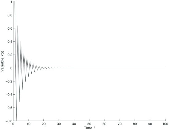
Figure 1 illustrates the simple equation
![]()
whose solution, with initial condition x1 = 1, is
![]()
The behavior of the solution is that of an exponential decay.
Figure 2 illustrates the equation
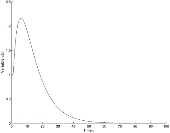
Figure 3 Solution of the Equation (1 − 1.7L + 0.72L2)xt = 0 with Initial Conditions x1 = 1, x2 = 1.5
![]()
Simulations were run for 100 time steps
whose solution, with initial condition x1 = 1, is
![]()
The behavior of the solution is that of an exponential decay with oscillations at each step. The oscillations are due to the change in sign of the exponential at odd and even time steps.
If the equation has more than one real root, then the solution is a sum of exponentials. Figure 3 illustrates the equation
![]()
whose solution, with initial condition x1 = 1, x2 = 1.5, is
![]()
The behavior of the solution is that of an exponential decay after a peak.
Figure 4 illustrates the equation
![]()
whose solution, with initial condition x1 = 1, x2 = 1.5, is
Figure 4 Solution of the Equation (1 − 1.9L + 0.88L2)xt = 0 with Initial Conditions x1 = 1, x2 = 1.5
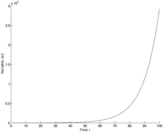
![]()
The behavior is that of exponential explosion due to the exponential with modulus greater than 1.
Complex Roots
Now suppose that some of the roots are complex. In this case, solutions exhibit an oscillating behavior with a period that depends on the model coefficients. For simplicity, consider initially a second-order homogeneous difference equation:
![]()
Suppose that its characteristic equation given by
![]()
admits the two complex conjugate roots:
![]()
Let’s write the two roots in polar notation:
It can be demonstrated that the general solution of the above difference equation has the following form:
![]()
where the C1 and C2 or C and ϑ are constants to be determined in function of initial conditions. If the imaginary part of the roots vanishes, then ω vanishes and a = r, the two complex conjugate roots become a real root, and we find again the expression xt = Crt.
Consider now a homogeneous difference equation of order 2n. Suppose that the characteristic equation has only two distinct complex conjugate roots with multiplicity n. We can write the difference equation as follows:
![]()
and its general solution as follows:
![]()
The general solution of a homogeneous difference equation that admits both real and complex roots with different multiplicities is a sum of the different types of solutions. The above formulas show that real roots correspond to a sum of exponentials while complex roots correspond to oscillating series with exponential dumping or explosive behavior. The above formulas confirm that in both the real and the complex case, solutions decay if the modulus of the roots of the inverse characteristic equation is outside the unit circle and explode if it is inside the unit circle.
Figure 5 illustrates the equation
![]()
which has two complex conjugate roots,
Figure 5 Solutions of the Equation (1 − 1.2L + 1.0L2)xt = 0 with Initial Conditions x1 = 1, x2 = 1.5
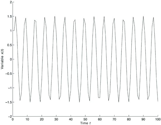
![]()
or in polar form,
![]()
and whose solution, with initial condition x1 = 1, x2 = 1.5, is
![]()
The behavior of the solutions is that of undamped oscillations with frequency determined by the model.
Figure 6 illustrates the equation
![]()
which has two complex conjugate roots,
![]()
or in polar form,
![]()
and whose solution, with initial condition x1 = 1, x2 = 1.5, is
Figure 6 Solutions of the Equation (1 − 1.0L + 0.89L2)xt = 0 with Initial Conditions x1 = 1, x2 = 1.5
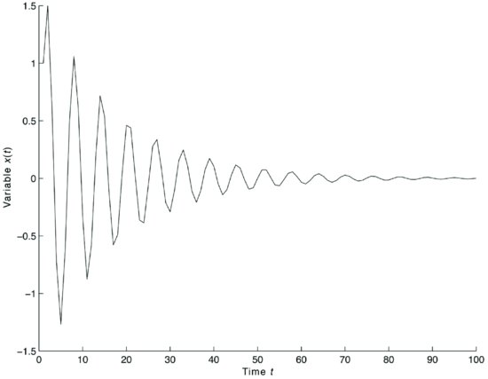
![]()
The behavior of the solutions is that of damped oscillations with frequency determined by the model.
NONHOMOGENEOUS DIFFERENCE EQUATIONS
Consider now the following n-th order difference equation:
![]()
where yt is a given sequence of real numbers. Recall that we are in a deterministic setting, that is, the yt are given. The general solution of the above difference equation will be the sum of two solutions x1,t + x2,t where x1,t is the solution of the associated homogeneous equation,
![]()
and X2,t solves the given nonhomogeneous equation.
Real Roots
To determine the general form of x2,t in the case of real roots, we begin by considering the case of a first-order equation:
![]()
We can compute the solution as follows:
which is meaningful only for |a1| < 1. If, however, yt starts at t = −1, that is, if yt = 0 for t = −2, −3, … , n, we can rewrite the above formula as
This latter formula, which is valid for any real value of a1, yields
and so on. These formulas can be easily verified by direct substitution. If yt = y = constant, then
![]()
Consider now the case of a second-order equation:
![]()
where λ1, λ2 are the solutions of the characteristic equation (the reciprocal of the solutions of the inverse characteristic equation). We can write the solution of the above equation as
![]()
Recall that, if |λi| < 1, i = 1, 2, we can write:
so that the solution can be written as
If the two solutions are coincident, reasoning as in the homogeneous case, we can establish that the general solutions can be written as follows:
If yt starts at t = −2, that is, if yt = 0 for t = −3, −4, … , −n, … , we can rewrite the above formula respectively as
if the solutions are distinct, and as
if the solutions are coincident. These formulas are valid for any real value of λ1.
The above formulas can be generalized to cover the case of an n-th order difference equation. In the most general case of an n-th order difference equation, assuming that all roots are real, there will be m < n distinct roots λi, i = 1, 2, … , m, each of order ni ≥ 1,
![]()
and the general solution of the process will be
if |λi| < 1, i = 1, 2, … , m, and
if yt starts at t = −n, that is, if yt = 0 for t = −(n + 1), −(n + 2), … for any real value of the λi.
Therefore, if the roots are all real, the general solution of a difference equation is a sum of exponentials. Figure 7 illustrates the case of the same difference equation as in Figure 3 with the same initial conditions x1 = 1, x2 = 1.5 but with an exogenous forcing sinusoidal variable:
Figure 7 Solutions of the Equation ![]() with Initial Conditions x1 = 1, x2 = 1.5
with Initial Conditions x1 = 1, x2 = 1.5
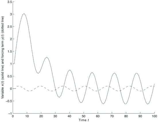
![]()
The solution of the equation is the sum of x1,t = −7.5(0.8)t + 7.7778(0.9)t plus
![]()
After the initial phase dominated by the solution of the homogeneous equation, the forcing term dictates the shape of the solution.
Complex Roots
Consider now the case of complex roots. For simplicity, consider initially a second-order difference equation:
![]()
Suppose that its characteristic equation,
![]()
admits the two complex conjugate roots,
![]()
We write the two roots in polar notation:
![]()
It can be demonstrated that the general form of the x2,t of the above difference equation has the following form:
![]()
which is meaningful only if |r| < 1. If yt starts at t = −2, that is, if yt = 0 for t = −3, −4, … , −n, … we can rewrite the previous formula as
![]()
This latter formula is meaningful for any real value of r. Note that the constant ω is determined by the structure of the model while the constants C1, C2 that appear in x1,t need to be determined in the function of initial conditions. If the imaginary part of the roots vanishes, then ω vanishes and a = r, the two complex conjugate roots become a real root, and we again find the expression xt = Crt.
Figure 8 illustrates the case of the same difference equation as in Figure 7 with the same initial conditions x1 = 1, x2 = 1.5 but with an exogenous forcing sinusoidal variable:
Figure 8 Solutions of the Equation (1 − 1.2L + 1.0L2)xt = 0.5 × sin(0.4 × t) with Initial Conditions x1 = 1, x2 = 1.5
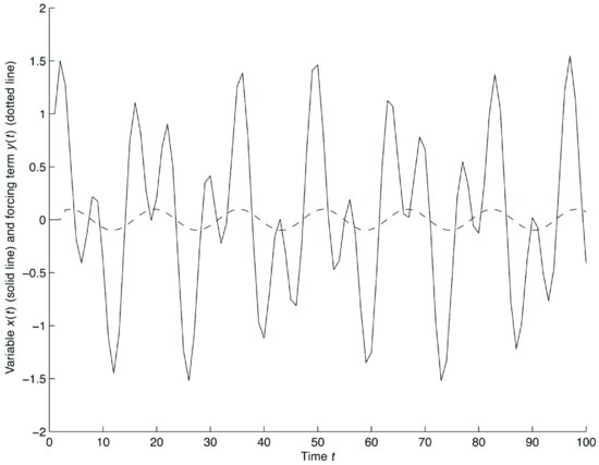
![]()
The solution of the equation is the sum of x1,t = −0.3cos(0.9273t) + 1.475 sin(0.9273t) plus
After the initial phase dominated by the solution of the homogeneous equation, the forcing term dictates the shape of the solution. Note the model produces amplification and phase shift of the forcing term 0.1 × sin(0.4 × t) represented by a dotted line.
SYSTEMS OF LINEAR DIFFERENCE EQUATIONS
In this section, we discuss systems of linear difference equations of the type
![]()
or in vector notation:
![]()
Observe that we need to consider only first-order systems, that is, systems with only one lag. In fact, a system of an arbitrary order can be transformed into a first-order system by adding one variable for each additional lag. For example, a second-order system of two difference equations,
can be transformed in a first-order system adding two variables:
Transformations of this type can be generalized to systems of any order and any number of equations.
A system of difference equations is called homogeneous if the exogenous variable yt is zero, that is, if it can be written as
![]()
while it is called nonhomogeneous if the exogenous term is present.
There are different ways to solve first-order systems of difference equations. One method consists in eliminating variables as in ordinary algebraic systems. In this way, the original first-order system in k equations is solved by solving a single difference equation of order k with the methods explained above. This observation implies that solutions of systems of linear difference equations are of the same nature as those of difference equations (i.e., sums of exponential and/or sinusoidal functions). In the following section we will show a direct method for solving systems of linear difference equations. This method could be used to solve equations of any order, as they are equivalent to first-order systems. In addition, it gives a better insight into vector autoregressive processes.
SYSTEMS OF HOMOGENEOUS LINEAR DIFFERENCE EQUATIONS
Consider a homogeneous system of the following type:
![]()
where A is a k × k, real-valued, nonsingular matrix of constant coefficients. Using the lag operator notation, we can also write the above systems in the following form:
![]()
If a vector of initial conditions x(0) is given, the above system is called an initial value problem.
Through recursive computation, that is, starting at t = 0 and computing forward, we can write

The following theorem can be demonstrated: Any homogeneous system of the type x(t) = Ax(t − 1), where A is a k × k, real-valued, nonsingular matrix, coupled with given initial conditions x(0) admits one and only one solution.
A set of k solutions xi(t), i = 1, … , k, t = 0, 1, 2, … are said to be linearly independent if
![]()
t = 0, 1, 2, … implies ci = 0, i = 1, … , k. Suppose now that k linearly independent solutions xi(t), i = 1, … , k are given. Consider the matrix
![]()
The following matrix equation is clearly satisfied:
![]()
The solutions xi(t), i = 1, … , n are linearly independent if and only if the matrix ![]() (t) is nonsingular for every value t ≥ 0, that is, if det[
(t) is nonsingular for every value t ≥ 0, that is, if det[![]() (t)] ≠ 0, t = 0, 1, …. Any nonsingular matrix
(t)] ≠ 0, t = 0, 1, …. Any nonsingular matrix ![]() (t), t = 0, 1, … such that the matrix equation
(t), t = 0, 1, … such that the matrix equation
![]()
is satisfied is called a fundamental matrix of the system x(t) = Ax(t − 1), t = 1, … , n, … and it satisfies the equation
![]()
In order to compute an explicit solution of this system, we need an efficient algorithm to compute the matrix sequence At. We will discuss one algorithm for this computation.1 Recall that an eigenvalue of the k × k real valued matrix A = (aij) is a real or complex number λ that satisfies the matrix equation:
![]()
where ![]() is a k-dimensional complex vector. The above equation has a nonzero solution if and only if
is a k-dimensional complex vector. The above equation has a nonzero solution if and only if
![]()
or
The above condition can be expressed by the following algebraic equation:
![]()
which is called the characteristic equation of the matrix A = (aij).
To see the relationship of this equation with the characteristic equations of single equations, consider the k-order equation:
![]()
which is equivalent to the first-order system,
The matrix

is called the companion matrix. By induction, it can be demonstrated that the characteristic equation of the system x(t) = Ax(t − 1), t = 1, … , n, … and of the k-order equation above coincide.
Given a system x(t) = Ax(t − 1), t = 1, … , n, … , we now consider separately two cases: (1) All, possibly complex, eigenvalues of the real-valued matrix A are distinct, and (2) two or more eigenvalues coincide.
Recall that if λ is a complex eigenvalue with corresponding complex eigenvector ξ, the complex conjugate number ![]() is also an eigenvalue with corresponding complex eigenvector
is also an eigenvalue with corresponding complex eigenvector ![]() .
.
If the eigenvalues of the real-valued matrix A are all distinct, then the matrix can be diagonalized. This means that A is similar to a diagonal matrix, according to the matrix equation
and
We can therefore write the general solution of the system x(t) = Ax(t − 1) as follows:
![]()
The ci are complex numbers that need to be determined for the solutions to be real and to satisfy initial conditions. We therefore see the parallel between the solutions of first-order systems of difference equations and the solutions of k-order difference equations that we have determined above. In particular, if solutions are all real they exhibit exponential decay if their modulus is less than 1 or exponential growth if their modulus is greater than 1. If the solutions of the characteristic equation are real, they can produce oscillating damped or undamped behavior with period equal to two time steps. If the solutions of the characteristic equation are complex, then solutions might exhibit damped or undamped oscillating behavior with any period.
To illustrate the above, consider the following second-order system:
![]()
This system can be transformed in the following first-order system:
with matrix
The eigenvalues of the matrix A are distinct and complex:
![]()
The corresponding eigenvector matrix Ξ is
Each column of the matrix is an eigenvector.
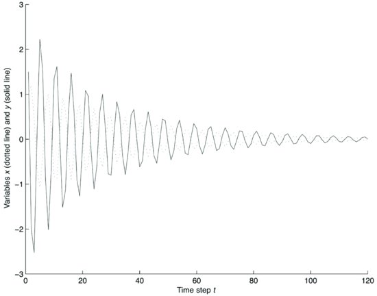
The solution of the system is given by
The four constants c can be determined using the initial conditions: (1) = 1; x(2) = 1.2; y(1) = 1.5; y(2) = −2. Figure 9 illustrates the behavior of solutions.
Now consider the case in which two or more solutions of the characteristic equation are coincident. In this case, it can be demonstrated that the matrix A can be diagonalized only if it is normal, that is if
![]()
If the matrix A is not normal, it cannot be diagonalized. However, it can be put in Jordan canonical form. In fact, it can be demonstrated that any nonsingular real-valued matrix A is similar to a matrix in Jordan canonical form,
![]()
where the matrix J has the form J = diag[J1, … , Jk], that is, it is formed by Jordan diagonal blocks:
where each Jordan block has the form
The Jordan canonical form is characterized by two sets of multiplicity parameters, the algebraic multiplicity and the geometric multiplicity. The geometric multiplicity of an eigenvalue is the number of Jordan blocks corresponding to that eigenvalue, while the algebraic multiplicity of an eigenvalue is the number of times the eigenvalue is repeated. An eigenvalue that is repeated s times can have from 1 to s Jordan blocks. For example, suppose a matrix has only one eigenvalue λ = 5 that is repeated three times. There are four possible matrices with the following Jordan representation:

These four matrices have all algebraic multiplicity 3 but geometric multiplicity from left to right 1, 2, 2, 3, respectively.
KEY POINTS
- Homogeneous difference equations are linear conditions that link the values of variables at different time lags.
- In the case of real roots, solutions are sums of exponentials. Any linear combination of solutions of the homogeneous difference equation is another solution.
- When some of the roots are complex, the solutions of a homogeneous difference equation exhibit an oscillating behavior with a period that depends on the model coefficients.
- The general solution of a homogeneous difference equation that admits both real and complex roots with different multiplicities is a sum of the different types of solutions.
- A system of difference equations is called homogeneous if the system’s exogenous variable is zero, and nonhomogeneous if the exogenous term is present.
- One method of solving first-order systems of difference equations is by eliminating variables as in ordinary algebraic systems; another way is a direct method that can be used to solve systems of linear difference equations of any order.
NOTE
1. This discussion of systems of difference equations draws on Elaydi (2002).
REFERENCES
Elaydi, S. (2002). An Introduction to Difference Equations. New York: Springer Verlag.
Goldberg, S. (2010). Introduction to Difference Equations. New York: Dover Publications.
Kelley, W. G., and Peterson, A. C. (1991). Difference Equations: An Introduction with Applications, 2nd ed. San Diego, CA: Academic Press.