
Robust Estimates of Betas and Correlations
Point estimates of betas and correlations are most often obtained using ordinary least squares (OLS) and the standard maximum likelihood estimator, respectively. While these estimators are clearly optimal when asset returns are normally distributed, and when we hold no view on their prior distribution, they can be far from optimal when these conditions are not satisfied. In this entry, a novel explanation of OLS is provided and is then used to motivate a robust univariate regression algorithm due to Theil (1950) and Sen (1968). This estimator is then used to obtain remarkably robust (i.e., outlier resistant) estimates of asset betas, asset correlations, and non-negative definite correlation and covariance matrices.
OLS REVISITED
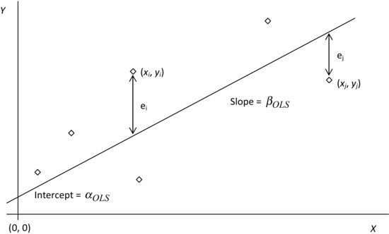
Generations of students have learned OLS in the way depicted pictorially in Figure 1. We are given a set of points, each with an abscissa (or x value) and an ordinate (or y value), and which are displayed on a scatter plot in the X − Y plane. All errors are assumed to be concentrated in the ordinates. The abcissae are assumed to be known with certainty. The ith point has coordinates (xi, yi), and the collection of points visually evidences a noisy, but linear, relationship between the x’s and the y’s. The object of OLS is to find a straight line, the line of best fit, with slope βOLS and intercept αOLS, and which minimizes the sum of squared vertical distances (or errors) from the points to this line.
Figure 1 Ordinary Least Squares—Classical Depiction
This pictorial representation has become so firmly embedded in our consciousness that we take its geometry and its formulation for granted. But consider that the method dates back to 1800, and the fact that it was independently discovered by Carl Friedrich Gauss and Joseph-Louis Lagrange, who surely rank among the greatest mathematicians of all time, and it should come as no surprise that this textbook depiction of OLS hides more than one secret. In this section, we expose two of its secrets.
Figure 2 Ordinary Least Squares—Alternative Depiction
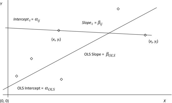
We start our exploration of OLS with Figure 2, which plots the same set of points as Figure 1, but now, instead of drawing a single line of best fit through the entire data set, we choose two specific points, (xi, yi) and (xj, yj), draw the unique straight line joining them and project it back till it intersects the Y axis. This line has slope βij and intercept αij, where βij and αij are given by:
(1) ![]()
and
(2) ![]()
On comparing Figures 1 and 2, it is clear that βOLS must necessarily lie between ![]() and
and ![]() , both endpoints inclusive, and that αOLS must likewise lie between
, both endpoints inclusive, and that αOLS must likewise lie between ![]() and
and ![]() . The OLS slope and intercept can therefore be written as weighted averages of all
. The OLS slope and intercept can therefore be written as weighted averages of all ![]() pairwise slopes and intercepts for some nonnegative sets of weights, that is,
pairwise slopes and intercepts for some nonnegative sets of weights, that is,
and
In any particular situation, these weights are not unique, as equations (3) and (4) are enormously overdetermined, and we therefore seek a set of strictly positive weights that simultaneously solves both equations for an arbitrary collection of points. Such a set of weights can be identified using some clever guesswork motivated by the following observation: If (xi, yi) and (xj, yj) are close together, then any error in either ordinate will induce significant errors in βij and αij. Pairs of points that are far apart are much less susceptible to this problem. We ought, therefore, to overweight slopes and intercepts derived from pairs of points that are far apart relative to those that are derived from pairs of points that are close together.
Next, as all the error is concentrated in the abscissae, and as the ordinates are known with certainty, the weights must be a function only of (xi−xj)—they cannot depend on (yi−yj). Finally, the function must be even, because some weights would be negative if it were odd. Some tedious and not particularly enlightening algebra shows our intuition to be correct, that is,
(5) 
It follows that
and
Equations (6) and (7) yield OLS’ first little secret—the line of best fit is just an appropriately weighted average of all possible lines that could be drawn using this data set! While this argument does not readily extend to the multivariate case, it does give us a fresh perspective on OLS, which now stands exposed as a clever and computationally efficient weighting scheme over the set of unique straight lines drawn through all possible pairs of points. A proof of this result, which is usually credited to Sen (1968), can be found in Heitman and Ord (1985).
Its second little secret lies in its focus on squared errors. Why should it be the second, and not the fourth or the sixty-fourth power of the error that is minimized? To answer this question, recall the way in which the OLS slope and intercept are defined:
(8) 
Solving this minimization problem requires us to compute the partial derivatives of the sum of squared errors with respect to αOLS and βOLS, and to equate the resulting expressions to 0. This results in a set of linear equations that can be solved in closed form (the solution was known to both Gauss and Lagrange). If, however, the error is raised to a power other than two, we would have to solve a set of nonlinear equations, which do not, in general, admit a closed form solution—they must be solved numerically on a computer, a tool that neither Gauss nor Lagrange had access to. That said, raising the error to any even power (or even making it the argument of any even function) and then performing the indicated minimization numerically will result in a line that is optimal under that measure, though its slope and intercept will not, in general, equal the OLS slope and intercept.
All of this leads to our second insight—the mathematical formulation of OLS is driven by thoroughly practical considerations. In 1800, anything else simply couldn’t be (and for that matter, still can’t be) solved analytically! Having exposed these two little secrets of OLS, we now describe a better way in which to compute univariate regressions and explore its application to the estimation of beta and the correlation coefficient, as well as to the estimation of positive definite correlation and covariance matrices.
THEIL-SEN REGRESSION
The Theil-Sen regression algorithm (Thiel, 1950; Sen, 1968) is a robust alternative to univariate OLS that performs particularly well in the presence of outliers (loosely, in the presence of large, sporadic errors that are anything but Gaussian). It has long been known that OLS is acutely sensitive to errors in its inputs, and it is immediately apparent from equations (6) and (7) that even a single outlier can induce arbitrarily large errors in βOLS and αOLS.
Theil (1950) and Sen (1968) propose a novel solution to this problem—they propose using the median of all ![]() slopes to estimate the slope of the regression line, and choose the intercept to force the median error to 0. The primary difference between their methods is that Theil uses all available observations, while Sen restricts attention to the subset of observations with distinct abscissae, that is, the set of points for which
slopes to estimate the slope of the regression line, and choose the intercept to force the median error to 0. The primary difference between their methods is that Theil uses all available observations, while Sen restricts attention to the subset of observations with distinct abscissae, that is, the set of points for which ![]() , and replaces each set of points that share the same abscissa with a single point whose ordinate is the average of their ordinates.
, and replaces each set of points that share the same abscissa with a single point whose ordinate is the average of their ordinates.
Formally, the Theil-Sen estimates of slope and intercept are given by:
(9) ![]()
and
(10) ![]()
This regression has been widely studied. Peng, Wang, and Wang (2008), for example, show that it is strongly consistent and superefficient, and derive its asymptotic distribution. Interestingly, the median has long been used as a robust estimator of the mean for symmetric distributions, but this appears to be the first known application of the median to the estimation of regression coefficients.
We illustrate the superiority of Thiel-Sen regression over OLS via simulations, the results of which are displayed in Tables 1 and 2. When the distribution of errors is normal, the distributions of βTS and αTS are almost identical to those of βOLS and αOLS. When the errors are drawn from a highly skewed distribution, or when the data are contaminated with significant amounts of noise, the distributions of βTS and αTS are far less variable than those of βOLS and αOLS.
Table 1 Theil-Sen Regression vs. OLS: Normally Distributed Random Variables
Table 2 Theil-Sen Regression vs. OLS: Pareto(2) Distributed Random Variables
These results are generated as follows. Using a high-quality random number generator (Mersenne twister), we create two independent random vectors, X and Y, both of length 100, and drawn from one of two distributions—unit normal and Pareto(2). We then regress Y against X using both OLS and the Theil-Sen regression. As the vectors are independent, the distribution of the slope and the intercept of the regression lines should be centered at 0 and E[X], respectively.
We run 10,000 simulations to ensure that the 99% confidence intervals on our estimates are extremely tight (the width of the confidence interval is inversely proportional to the square root of the number of simulation runs), and Tables 1 and 2 display various percentiles of the distribution of the slope, the intercept, and the mean squared error (i.e., the sum of squared errors divided by 100) for both OLS and the Theil-Sen regression.
The first simulation, for normal random variables, illustrates how close the Theil-Sen algorithm is to OLS in the special case when OLS is clearly optimal. The second simulation illustrates its robustness with Pareto(2) random variables, whose distribution is highly skewed, and whose long tails serve as proxies for outliers.
When X and Y are normally distributed (Table 1), the median slope, the interquartile range for the slope (the difference between the 75th and the 25th percentiles), and the MSE for the two algorithms are essentially identical. The same holds true even when we look at a 90% range (the difference between the 5th and the 95th percentiles). However, when X and Y are drawn from a Pareto(2) distribution (Table 2), the performance of the two algorithms diverges: The interquartile range for the slope is 40% smaller for the Theil-Sen regression (0.06 vs. 0.10 for OLS) and an astonishing 60% smaller for the 90% range (0.16 vs. 0.41), though the median MSE rises by about 12%.
The median slope remains 0 for the Theil-Sen regression, but exhibits a slight downward bias for OLS. The range of the intercept for the Thiel-Sen regression is slightly larger than it is for OLS, but this is driven entirely by the fact that the Theil-Sen intercept is chosen to force the median error to 0, while the OLS intercept is chosen to minimize the sum of squared errors.
These simulations clearly show that the Theil-Sen regression gives up nothing to OLS when X and Y are normally distributed and is at a significant advantage when they are not. Similar results are obtained when either X or Y is contaminated with outliers. In all such experiments, the advantage of the Theil-Sen approach is readily apparent. In fact, it can be shown that as many as 29% of the data points can be corrupted with errors of arbitrary size before the Theil-Sen estimates of slope and intercept start to break down.
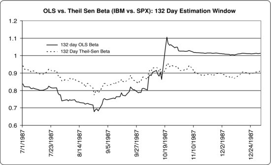
Figure 3 OLS vs. Theil-Sen Estimates of Beta: July 1, 1987, to December 31, 1987
Given these results, and the accompanying fact that the vast majority of regressions run in practice are univariate, it is surprising that the Theil-Sen regression is not more widely used and appreciated. This may in part be driven by the fact that Theil-Sen regression, unlike OLS, does not generalize naturally to the case where there are many independent variables, as the median is inherently a one-dimensional measure.
A number of attempts have been made to create multivariate extensions of the Theil-Sen regression, the two most popular ones being the iterative Gauss-Seidel method described by Hastie and Tibshirani (1990) and the elemental subset method of Oja and Niinimaa (1984), which is described in Rousseeuw and Leroy (1987). Unfortunately, neither approach is entirely reliable in practice, and it is easy to find simple examples for which they converge to the wrong solution, particularly when the relationship being modeled is nonlinear.
ROBUST ESTIMATES OF BETA
The beta of an asset Y with respect to the market portfolio X plays a central role in modern finance as a result of the capital asset pricing model (Treynor, 1961; Sharpe, 1964; Lintner, 1965; and Mossin, 1966), and is defined to be
(11) ![]()
This quantity is, of course, just the slope coefficient in a univariate regression, and is precisely what OLS estimates. The application of the Theil-Sen regression algorithm to the estimation of beta is obvious—the Theil-Sen estimate of slope ought to provide us a more robust estimate of the historical of a security than the corresponding OLS estimate.
The advantages of the Theil-Sen estimator of beta are made clear by the following estimate of the beta of IBM around the crash of 1987. Starting on July 1, 1987, and ending on December 31, 1987, we estimate IBM’s β by regressing its daily return for the most recent 132 days (or 6 months) against the corresponding daily return of the S&P 500. As can be seen from Figure 3, the Theil-Sen estimate is far more stable than the OLS estimate. In particular, it does not jump sharply after the 20% drop in the S&P 500 on October 19 as does the OLS beta, just as one would expect given its robustness.
While this is clearly an extreme example of a single outlier corrupting an estimate of beta, outliers in financial data are far more common than is usually assumed, and they are not easily detected, as they influence many classical estimators in a way that masks their presence. One popular method of identifying and removing outliers is to remove points that lie more than three sample standard deviations away from the regression line.
Unfortunately, outliers can so distort the slope and intercept of the regression line, as well as the sample standard deviation of the errors, that all the points, including the outliers, will be found to lie within three sample standard deviations of the regression line! In general, filtering data using classical estimators to identify outliers works poorly in practice, and it proves far more effective to use estimators that are inherently robust to outliers.
The Theil-Sen estimate of beta can be further adjusted for the effects of nonsynchronous trading using the Scholes-Williams (1977) or Dimson (1979) corrections and can be shrunk cross-sectionally using a Bayesian correction as is done in Vasicek (1973). In each case, the Theil-Sen estimates of beta will provide a more robust point from which to start building an enhanced estimate of beta.
The Dimson correction sums contemporaneous and lagged betas for the asset to create an overall beta that accounts for the fact that an asset may have both a contemporaneous and a lagged response to market shocks, that is,
(12) ![]()
When using daily data, k is commonly set to 4 (i.e., one week’s data), and when using monthly data, it is most commonly set to 1, so as not to pick up spurious responses from shocks in the distant past.
Vasicek’s (1973) correction is a Bayesian correction, which allows the user to reflect information gleaned from the (known) cross-sectional distribution of betas to enhance an unconditional estimate of beta. In particular, Vasicek (1973) assumes that the prior distribution of betas is normal and shows that the maximum a posteriori estimate of beta is a linear combination of its initial estimate and its cross-sectional mean, that is,
(13) ![]()
where
(14) ![]()
![]() is the variance of βY|X, and
is the variance of βY|X, and ![]() is the cross-sectional variance of the betas of the entire universe of securities under consideration at this point in time. A particularly simple and reasonably effective implementation of this method sets wY = 0.5 for all assets and at all points in time. Both techniques see use in the enhanced estimation of beta across a wide range of asset classes in Frazzini and Pedersen (2010).
is the cross-sectional variance of the betas of the entire universe of securities under consideration at this point in time. A particularly simple and reasonably effective implementation of this method sets wY = 0.5 for all assets and at all points in time. Both techniques see use in the enhanced estimation of beta across a wide range of asset classes in Frazzini and Pedersen (2010).
ROBUST ESTIMATES OF CORRELATION
To derive a robust estimate of the correlation coefficient, we rewrite and re-interpret the expression for the correlation coefficient in a novel way, and then show how it can be estimated using two Theil-Sen regressions. Recall the definition of the correlation between two random variables X and Y:
(15) ![]()
where ![]() is the covariance between X and Y, and
is the covariance between X and Y, and ![]() and
and ![]() are the standard deviations of X and Y, respectively. This expression can be rewritten as
are the standard deviations of X and Y, respectively. This expression can be rewritten as
Factored in this way, the correlation coefficient stands revealed as the geometric mean of two betas and is interpreted as follows. If a causal linear relationship runs from X to Y, (i.e., if X causes Y), the logical quantity to focus on is βY|X. Likewise, if a causal linear relationship runs from Y to X, (i.e., if Y causes X), the logical quantity to focus on is βX|Y.
Table 3 Distribution of Theil-Sen Estimates of Correlation vs. Standard Maximum Likelihood Estimate: Normally Distributed Random Variables
Table 4 Distribution of Theil-Sen Estimates of Correlation vs. Standard Maximum Likelihood Estimate: Pareto(2) Distributed Random Variables
But when we don’t know which way the causation flows, or even if the relationship is linear, we throw our hands up, take the geometric mean of these two betas, and call this quantity the correlation coefficient! For jointly normally distributed random variables, the correlation coefficient fully captures and encapsulates their covariation. For all other distributions, it serves merely as a useful shortcut that measures their covariation in a standardized way, as evidenced by the fact that its value is bounded between −1 and 1.
The application of the Theil-Sen regression to the robust estimation of correlation is now obvious. Given two random vectors, X and Y, first regress X on Y, and then regress Y on X, using the Theil-Sen regression both times. The geometric mean of the two slopes is a robust estimate of the correlation coefficient, that is,
(17) ![]()
When the random vectors are drawn from a normal distribution and are not corrupted by noise, we expect that this approach will work just as well as the standard maximum likelihood estimator. In the presence of outliers, or if distribution of X and Y is highly skewed, it ought to do much better. And so it is, as the data in Tables 3 and 4 demonstrate.
Table 3 compares the performance of equation (16) to the standard maximum likelihood estimator when X and Y are drawn from a normal distribution, while Table 4 performs an identical comparison for Pareto(2) random variables. Both tables are created by extending the simulations used to illuminate the performance of the Theil-Sen regression to compute correlations as well.
The results follow the pattern established in Tables 1 and 2 for the slope coefficient. When X and Y are drawn from a normal distribution, the distribution of the Theil-Sen estimate of correlation is essentially identical to that of the maximum likelihood estimate; and when they are drawn from a Pareto(2) distribution, the Theil-Sen estimate of correlation is far more stable than the maximum likelihood estimate. Similar results are obtained when either X or Y (or both) are contaminated with noise (i.e., with outliers).
It is a short step from estimating individual correlations to estimating correlation matrices, and the repeated use of the Theil-Sen estimator across a set of random variables gives us a computationally inefficient but robust estimate of a correlation matrix ![]() , whose i,jth element is denoted by
, whose i,jth element is denoted by ![]() , and whose diagonal elements are all 1. Unfortunately, there is no guarantee that this correlation matrix will be nonnegative definite.
, and whose diagonal elements are all 1. Unfortunately, there is no guarantee that this correlation matrix will be nonnegative definite.
This, however, is no cause for alarm. It is relatively easy to transform this matrix into a nearby nonnegative definite correlation matrix ![]() . Ideally, the transformation will minimally distort
. Ideally, the transformation will minimally distort ![]() , and the many available solutions to this problem differ largely in the metric (or norm) that they use to measure the distance between
, and the many available solutions to this problem differ largely in the metric (or norm) that they use to measure the distance between ![]() and
and ![]() . In general, they solve the following optimization problem:
. In general, they solve the following optimization problem:
(18) ![]()
Lindskog (2000), Rousseeuw and Molenberghs (1993), and Higham (2002) describe a number of different ways in which the nearest correlation matrix can be identified using both linear and nonlinear transformations of ![]() . The method that seems to work best in practice is the iterative method described by Higham (2002), which iteratively identifies the closest valid correlation matrix under a Frobenius norm (the sum of squared element by element differences) by factoring the correlation matrix in a particular way, forcing its negative eigenvalues to 0, then recombining its constituent pieces and forcing its diagonal elements to 1. The algorithm is described here for the sake of completeness and can be found in the NAG Fortran and C Libraries, as well as the NAG Toolbox for Matlab.
. The method that seems to work best in practice is the iterative method described by Higham (2002), which iteratively identifies the closest valid correlation matrix under a Frobenius norm (the sum of squared element by element differences) by factoring the correlation matrix in a particular way, forcing its negative eigenvalues to 0, then recombining its constituent pieces and forcing its diagonal elements to 1. The algorithm is described here for the sake of completeness and can be found in the NAG Fortran and C Libraries, as well as the NAG Toolbox for Matlab.
We first define two operators, PS(A) and PU(A) that can be applied to any symmetric matrix A. As A is symmetric, it admits a spectral decomposition ![]() , where Q is orthogonal, and
, where Q is orthogonal, and ![]() is a square matrix whose diagonal elements are the eigenvalues of A, and whose off-diagonal elements are 0. PS(A) and PU(A) are defined via
is a square matrix whose diagonal elements are the eigenvalues of A, and whose off-diagonal elements are 0. PS(A) and PU(A) are defined via
(19) ![]()
(20) ![]()
The algorithm proceeds as follows, with both Xk and Yk converging linearly to ![]() :
:
Algorithm H (Higham, 2002)
It is but a short step from estimating a robust nonnegative definite correlation matrix to estimating a similarly robust nonnegative definite covariance matrix. Given robust estimates of the volatility of each security, say ![]() , we can form a matrix whose diagonal elements are the robust volatilities of the assets, and whose off-diagonal elements are all 0, that is,
, we can form a matrix whose diagonal elements are the robust volatilities of the assets, and whose off-diagonal elements are all 0, that is,
(21) 
and we can then define a robust nonnegative definite covariance matrix ![]() via:
via:
If the correlation matrix is nonnegative definite, the covariance matrix described in equation (22) is nonnegative definite as well. Rousseeuw and Croux (1993) describe a number of robust estimators of volatility, their preferred one being QN(X), which is defined to be 2.222 times the 25th percentile of the set of distances {|xi−xj|, i<j}. They explore the properties of this estimator, which is similar in spirit to the Hodges–Lehmann (1963) estimate of the mean, show that its efficiency for the normal distribution is high (82%), and that it is robust to errors of arbitrary size in approximately half the points.
The robust covariance matrix defined by equation (22) can be used in a variety of applications such as mean-variance portfolio analysis and risk budgeting. It proves remarkably useful in practice, as it reduces and often completely eliminates the need for various constraints to ensure positive solutions that accord with a thoughtful portfolio manager’s intuition.
KEY POINTS
- The Theil-Sen regression algorithm is an extraordinarily simple, intuitive, and robust algorithm for performing univariate regressions.
- The Theil-Sen estimator should be used routinely in place of OLS when performing univariate regressions, and in place of the standard maximum likelihood estimator when estimating correlations.
- The fact that the Theil-Sen estimator does not generalize naturally to multivariate regression should not be held against it—the vast majority of regressions that are carried out in practice are univariate, and a wide range of robust algorithms that work well with multivariate data are known.
- The Theil-Sen regression algorithm can be used to obtain robust estimates of beta, which can be further enhanced by the application of Dimson’s correction for nonsynchronous trading and Vasicek’s Bayesian adjustment.
- The robust estimates of correlation obtained from the Theil-Sen regression algorithm can be used as inputs to Higham’s projection algorithm to estimate a nonnegative definite correlation matrix. This nonnegative definite correlation matrix can be combined with Rousseeuw and Croux’s robust estimator of volatility to estimate a nonnegative definite covariance matrix. This nonnegative definite covariance matrix is of particular use in a wide range of mean-variance portfolio optimization and risk budgeting applications, including, but not limited to, the construction of minimum variance portfolios.
REFERENCES
Dimson, E. (1979). Risk measurement when shares are subject to infrequent trading. Journal of Financial Economics 7, 2: 197–226.
Frazzini, A., and Pedersen, L. (2010). Betting against beta. http://papers.ssrn.com/sol3/papers.cfm?abstract_id=1723048
Hastie, T. J., and Tibshirani, R. J. (1990). Generalized Additive Models. New York: Chapman and Hall.
Heitman, G., and Ord, K. J. (1985). An interpretation of the least squares regression surface. The American Statistician 39, 2: 120--123.
Higham, N. (2002). Computing the nearest correlation matrix—a problem from finance. IMA Journal of Numerical Analysis, 22, 3: 329–343.
Hodges, J. L., Jr., and Lehmann, E. L. (1963). Estimates of location based on rank tests. Annals of Mathematical Statistics 34, 2: 598–611.
Linkdskog, F. (2000). Linear correlation estimation. http://www.risklab.ch/ftp/papers/LinearCorrelationEstimation.pdf
Lintner, J. (1965). The valuation of risky assets and the selection of risky investments in stock portfolios and capital budgets. Review of Economics and Statistics 47, 1: 13–37.
Mossin, J. (1966). Equilibrium in a capital asset market. Econometrica 34, 4: 768–783.
Oja, H., and Niinimaa, A. (1984). On Robust Estimation of Regression Coefficients. Research Report, Department of Applied Mathematics and Statistics, University of Oulu, Finland.
Peng, H., Wang, S., and Wang, X. (2008). Consistency and asymptotic distribution of the Theil-Sen estimator. Journal of Statistical Planning and Inference 138, 6: 1836–1850.
Rousseeuw, P. J., and Croux, C. (1993). Alternatives to the median absolute deviation. Journal of the American Statistical Association 88, 424: 1273–1283.
Rousseeuw, P. J., and Leroy, A. M. (1987). Robust Regression and Outlier Detection. New York: John Wiley and Sons.
Rousseeuw, P. J., and Molenberghs, G. (1993). Transformation of nonpositive semidefinite correlation matrices. Communications in Statistics—Theory and Methods 22, 4: 965–984.
Scholes, M., and Williams, J. (1977). Estimating betas from nonsynchronous data. Journal of Financial Economics 5, 3: 309–327.
Sen, P. K. (1968). Estimate of the regression coefficient based on Kendall’s Tau. Journal of the American Statistical Association 63, December: 1379–1389.
Sharpe, W. F. (1964). Capital asset prices: A theory of market equilibrium under conditions of risk. Journal of Finance 19, 3: 425–442.
Theil, H. (1950). A rank-invariant method of linear and polynomial regression analysis. Indigationes Mathematicae 12: 85–91.
Treynor, J. L. (1961). Towards a theory of market value of risky assets. Unpublished manuscript.
Vasicek, O. A. (1973). A note on using cross-sectional information in Bayesian estimation on security betas. Journal of Finance 28, 5: 1233–1239.