
Partial Differential Equations in Finance
Numerical methods based on partial differential equations (PDEs) in finance are not very popular. Indeed, the models are usually derived from probabilistic arguments and Monte Carlo methods are therefore much more natural. Stochastic methods are also often simpler to implement than the algorithms used for solving the related PDEs. However, when it is possible to efficiently discretize the PDE (which is not always the case, the typical counterexample being high-dimensional problems), deterministic methods are usually more efficient than stochastic ones. Moreover, the solution to the partial differential equation gives more information. In the context of option pricing, one obtains, for example, the price of the option for all values of the maturity and for all spot prices, while the probabilistic formulation typically gives the value of the option for a fixed maturity and a fixed spot price. In particular, this is useful for computing derivatives of the option’s price with respect to some parameters of the model (the so-called “Greeks”).
The PDEs obtained in finance have several characteristics. First, they are posed on a bounded domain in time (0, T), with typically a singular final condition at the maturity t = T, and very often in an unbounded domain in the spot variable, which requires to impose suitable “boundary conditions” at infinity to get well-posed problems and to use appropriate numerical approximations (truncation to a bounded domain and artificial boundary conditions). These PDEs are usually of parabolic type, but often with degenerate diffusions. Because of operational constraints, the numerical methods used for the discretization of the PDE must be sufficiently fast and accurate to be useful in practice. These peculiarities of PDEs in finance explain the need for up-to-date and sometimes involved numerical methods.
In this entry we focus on numerical issues and try to review the main numerical methods used for solving PDEs in finance. This presentation heavily relies on Achdou and Pironneau (2005), as well as Lamberton and Lapeyre (1997), Karatzas and Shreve (1991), and Wilmott, Dewynne, and Howison (1993).
PARTIAL DIFFERENTIAL EQUATIONS FOR OPTION PRICING
In this section, we present the main arguments to derive a PDE for the price of various European and American options.
A Primer: The Black and Scholes Model for European Options
The aim of this section is to recall the basic tools needed to derive a PDE in the context of option pricing, without providing all the detailed assumptions required on the data to perform this derivation. Karatzas and Shreve (1991) and Lamberton and Lapeyre (1997), for example, provide more details on the mathematical aspects. We adopt the standard Black and Scholes model (Black and Scholes, 1973; Merton, 1973) with a risky asset whose price at time t is St and a risk-free asset whose price at time t is S0t, such that:
![]()
The process Bt is a standard Brownian motion defined on a probability space ![]() , and μ (the mean rate of return), r (the interest rate), and σ > 0 (the volatility) are three constants. However, the following can be generalized to the case where μ, r, and σ > 0 are functions of t and S (under suitable smoothness assumptions).
, and μ (the mean rate of return), r (the interest rate), and σ > 0 (the volatility) are three constants. However, the following can be generalized to the case where μ, r, and σ > 0 are functions of t and S (under suitable smoothness assumptions).
We introduce the stochastic process ![]() . Under the so-called risk-neutral probability
. Under the so-called risk-neutral probability ![]() defined by its Radon-Nikodym derivative with respect to
defined by its Radon-Nikodym derivative with respect to ![]() by
by
Wt is a Brownian motion and St/S0t is a martingale. This is one of the fundamental properties of the stochastic process needed in the following. The process St satisfies the following stochastic differential equation (SDE) under ![]() :
:
Let us now consider a portfolio with Ht risky assets and H0t no-risk assets. Its value at time t is:
(2) ![]()
We suppose that this portfolio is self-financing (any manipulation on this portfolio, i.e., any change of the values of Ht or H0t, is done without any inflows or outflows of money), which translates into
The value of a self-financing portfolio changes if and only if the price of the risky asset changes. Using (3), it is possible to show that Pt/S0t is also a martingale.
We consider the following problem: For a given function ![]() (the payoff function) and a given time T>0 (the maturity), is it possible to build a self-financing portfolio such that
(the payoff function) and a given time T>0 (the maturity), is it possible to build a self-financing portfolio such that ![]() Classical examples of function
Classical examples of function ![]() are
are ![]() (vanilla call) or
(vanilla call) or ![]() (vanilla put), where, for any real x, x+ = max(x, 0) and x− = max(−x, 0). The answer is positive (this is typically based on a martingale representation theorem, the fact that Pt/S0t is a martingale, and the fact that the payoff
(vanilla put), where, for any real x, x+ = max(x, 0) and x− = max(−x, 0). The answer is positive (this is typically based on a martingale representation theorem, the fact that Pt/S0t is a martingale, and the fact that the payoff ![]() is
is ![]() -measurable), and it is then possible to show that such a portfolio has the following value at time t:
-measurable), and it is then possible to show that such a portfolio has the following value at time t:
where here and in the following, ![]() denotes an expectation with respect to the risk-neutral probability
denotes an expectation with respect to the risk-neutral probability ![]() . By the so-called arbitrage-free principle, Pt is actually the “fair price” at time t of the option, which enables its owner to get the payoff
. By the so-called arbitrage-free principle, Pt is actually the “fair price” at time t of the option, which enables its owner to get the payoff ![]() at time T. In the particular context of vanilla options, the solution is analytically known, at least if r and σ are constant: This is the celebrated Black and Scholes formula. However, in the case when r and σ are functions of t and S, (4) cannot be estimated without a numerical method. We are interested in deterministic numerical methods, based on a PDE related to (4).
at time T. In the particular context of vanilla options, the solution is analytically known, at least if r and σ are constant: This is the celebrated Black and Scholes formula. However, in the case when r and σ are functions of t and S, (4) cannot be estimated without a numerical method. We are interested in deterministic numerical methods, based on a PDE related to (4).
The second fundamental property of the stochastic process St required to obtain a PDE formulation of this problem is a Markov property. Roughly speaking, it states that the expectation of any function of ![]() conditionally to
conditionally to ![]() is actually a function of the price St of the risky asset at time t. In our context, this property shows that Pt writes
is actually a function of the price St of the risky asset at time t. In our context, this property shows that Pt writes
where p is a function of ![]() and
and ![]() , called the pricing function of the option. Notice that even if (5) only involves the value of p at point (t, St), the pricing function p is a deterministic function defined for all values of
, called the pricing function of the option. Notice that even if (5) only involves the value of p at point (t, St), the pricing function p is a deterministic function defined for all values of ![]() and
and ![]() . By the Markov property of St, we also have the following representation formula for p:
. By the Markov property of St, we also have the following representation formula for p:
where ![]() denotes the process solution to (1) starting from x at time t
denotes the process solution to (1) starting from x at time t
(7) ![]()
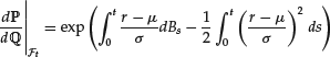
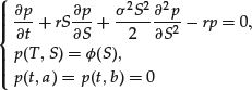
By using Ito’s calculus and the fact that Pt/S0t is a martingale, we then obtain that p should satisfy the following backward-in-time PDE:
Conversely, it is possible (using again a martingale representation theorem) to show that if p satisfies (8), then p(t, St) is the value of a self-financing portfolio with value ![]() at time T. Moreover, one can check that
at time T. Moreover, one can check that ![]() , which shows that obtaining an accurate approximation of
, which shows that obtaining an accurate approximation of ![]() is important in order to estimate the quantity of risky asset Ht needed at time t to build the portfolio with value Pt (this is the hedging strategy). Collectively, equations (4) – (5) and (8) provide an example of so-called Feynman-Kac formulas, which are used in many other contexts (quantum chemistry or transport equations, for example) either to give a probabilistic interpretation to a PDE, or to recast the computation of an expectation into a PDE problem.
is important in order to estimate the quantity of risky asset Ht needed at time t to build the portfolio with value Pt (this is the hedging strategy). Collectively, equations (4) – (5) and (8) provide an example of so-called Feynman-Kac formulas, which are used in many other contexts (quantum chemistry or transport equations, for example) either to give a probabilistic interpretation to a PDE, or to recast the computation of an expectation into a PDE problem.
For problem (8) to be well posed (i.e., for one and only one solution to exist), one needs to supply the system with “boundary conditions” when S = 0 or ![]() . More precisely, one needs to make precise in which functional space the function p is looked for. This will be explained in the next section.
. More precisely, one needs to make precise in which functional space the function p is looked for. This will be explained in the next section.
From the PDE (8) and the so-called maximum principle, it is possible to derive many qualitative properties and a priori bounds on the price p (like the call-put parity, for example; see Achdou and Pironneau, 2005). Roughly speaking, the maximum principle states that if the data (initial condition, boundary conditions, right-hand side) for the PDE (8) are positive, then the solution is positive. This property is definitely necessary to hold for a price. It is also an important property to check on the numerical schemes (which is then called a discrete maximum principle as discussed below).
It is also possible to obtain the PDE without introducing the risk-neutral probability (see Wilmott, Dewynne, and Howison, 1993) by considering a portfolio containing some options and some risky assets and by using an arbitrage-free argument.
It is important to recall that the Black and Scholes model for the evolution of the risky asset (1) badly compares with experimental data. We discuss later in this entry some possible refinements that have been introduced in order to better fit the observations (see the discussion on calibration below). However, this model remains very important in practice because it is used as a prototypical description of the evolution of the asset. Moreover, for a given observed price of a derivative, there exists a constant volatility σ (called the implied volatility; see the section on calibration below) for which the Black-Scholes price is the observed price. The implied volatility is a major quantity used in practice to compare derivatives.
Other Options
The argument presented for the Black-Scholes model is prototypical. In particular, the derivation of a PDE satisfied by the pricing function of an option always relies on the two fundamental properties stressed above: the martingale and the Markov properties of a suitable stochastic process. In this section, we present PDEs for the prices of various options without providing all the details of the derivation.
Basket Options
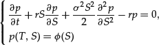
In many cases, the payoff of the option depends on the values of more than one asset, which typically do not evolve independently. Let us, for example, consider the case of two assets, which evolve following the following SDE under the neutral risk probability
where W1t and W2t are possibly correlated standard Brownian motions. We call ρ the correlation of W1t and W2t : ![]() . We suppose that the maturity is T>0 and the payoff is
. We suppose that the maturity is T>0 and the payoff is ![]() , where
, where ![]() is a given function. It is then possible to show that the price of the option at time t is p(t, S1t, S2t) where p satisfies
is a given function. It is then possible to show that the price of the option at time t is p(t, S1t, S2t) where p satisfies
Here again, r, σ 1, and σ 2 may be functions of t and (S1, S2). It is possible to solve such PDEs by standard numerical methods up to dimension 3 or 4. As discussed later, to derive appropriate discretization for higher dimensions is not an easy task and is still the subject of current research.
Barrier Options
Again, let us consider an option on a single asset. For some options, the payoff becomes 0 if there exists a time ![]() such that St goes below a or above b, where a and b are two given values, 0<a<b (the case a = 0 or
such that St goes below a or above b, where a and b are two given values, 0<a<b (the case a = 0 or ![]() can be treated similarly). Mathematically, the payoff is
can be treated similarly). Mathematically, the payoff is ![]() where, for any event
where, for any event ![]() , 1A denotes the characteristic function of A, and St satisfies (1). In this case, the relevant stochastic process for deriving the PDE is
, 1A denotes the characteristic function of A, and St satisfies (1). In this case, the relevant stochastic process for deriving the PDE is ![]() , where
, where ![]() is a stopping time, and, for any real x and y,
is a stopping time, and, for any real x and y, ![]() . It can be checked that
. It can be checked that ![]() is a Markov process, and that
is a Markov process, and that ![]() is a martingale. It is then possible to show that the price of the option at time t is
is a martingale. It is then possible to show that the price of the option at time t is ![]() where p is defined for
where p is defined for ![]() and
and ![]() and satisfies:
and satisfies:
(10) 
Here again, r and σ may be functions of t and S. Moreover, the generalization to basket options is straightforward, as explained above. In this case, it is possible to consider more general barriers, namely a payoff of the form ![]() , where d denotes the number of underlying assets and
, where d denotes the number of underlying assets and ![]() is any simple connected domain of
is any simple connected domain of ![]() . The appropriate discretization for general domains
. The appropriate discretization for general domains ![]() is the finite element method that will be discussed later on.
is the finite element method that will be discussed later on.
Options on the Maximum
For some options (the so-called lookback options), the payoff involves the maximum of the risky asset. For example, it writes ![]() where
where ![]() and St satisfies (1). One can check that (St, Mt) is a Markov process. It is then possible to show that the price of the option at time t is p(t, St, Mt) where p is defined for
and St satisfies (1). One can check that (St, Mt) is a Markov process. It is then possible to show that the price of the option at time t is p(t, St, Mt) where p is defined for ![]() and
and ![]() and satisfies:
and satisfies:
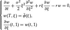
If the payoff is of the form ![]() , it is possible to reduce the problem to a two-dimensional one (including the time variable). Indeed, one can check by straightforward computations that p(t, S, M) = Mw(t, S/M) where w is a function of
, it is possible to reduce the problem to a two-dimensional one (including the time variable). Indeed, one can check by straightforward computations that p(t, S, M) = Mw(t, S/M) where w is a function of ![]() and
and ![]() , which satisfies:
, which satisfies:
(12) 
Notice that this reduction is not generally possible for (t, S, M)-dependent interest rate and volatility (except for very peculiar dependencies).
Options on the Average
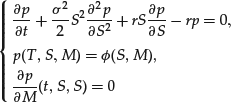
Some options (the so-called Asian options) involve the average of the risky asset. More precisely, the payoff writes ![]() where
where ![]() and St satisfies (1). One can check that (St, At) is a Markov process. Using this property, it is possible to show that the price of the option at time t is p(t, St, At) where p is defined for
and St satisfies (1). One can check that (St, At) is a Markov process. Using this property, it is possible to show that the price of the option at time t is p(t, St, At) where p is defined for ![]() and
and ![]() , and p satisfies:
, and p satisfies:
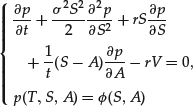
In some cases (see Rogers and Shi, 1995), it is possible to reduce this problem to a one-dimensional PDE. More precisely, for fixed strike call (![]() ) or fixed strike put (
) or fixed strike put (![]() ), we have
), we have ![]() where f satisfies
where f satisfies
and ![]() (resp.
(resp. ![]() ). This reduction of (13) to (14) is also possible for floating strike call (
). This reduction of (13) to (14) is also possible for floating strike call (![]() ) (resp. for floating strike put (
) (resp. for floating strike put (![]() )) by setting
)) by setting ![]() and
and ![]() (resp.
(resp. ![]() ). However, this reduction is generally not possible for general payoff function or (t, S, A)-dependent interest rate and volatility (except for very peculiar dependencies).
). However, this reduction is generally not possible for general payoff function or (t, S, A)-dependent interest rate and volatility (except for very peculiar dependencies).
Bermudean Options
As a transition between European and American options, we would like to mention that it is very easy to price Bermudean options with the PDE approach. For such options, the contract can be exercised only at certain days between the present time and the maturity. Mathematically, for an option on a single asset (the spot price is called S) and if ![]() denotes the payoff, the pricing function satisfies
denotes the payoff, the pricing function satisfies ![]() , at each exercising time ti, and (8) between the exercising times; see Duffie (1992, p. 211).
, at each exercising time ti, and (8) between the exercising times; see Duffie (1992, p. 211).
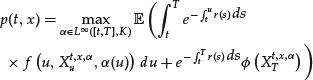
The Case of American Options
We have so far presented so-called European options, that is, some options that enable their owners to get ![]() at a fixed time T. On the other hand, American options can be exercised at any time up to the maturity. Hence the price of an American option of payoff
at a fixed time T. On the other hand, American options can be exercised at any time up to the maturity. Hence the price of an American option of payoff ![]() and maturity T will be the maximum of all possible expectations such as (6) for stopping times
and maturity T will be the maximum of all possible expectations such as (6) for stopping times ![]() between t and T, that is, for
between t and T, that is, for ![]() and
and ![]() ,
,
where ![]() denotes the set of stopping times
denotes the set of stopping times ![]() of the filtration
of the filtration ![]() , with values in [t, T].
, with values in [t, T].
The PDE for American Options
We now present the main arguments to derive a PDE on p defined by (15) (or more precisely a system of partial differential inequalities).
Notice first that taking ![]() in (15) yields the inequality
in (15) yields the inequality
Moreover, we clearly have from (15) ![]() .
.
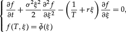
Let t and δt be such that ![]() . From (15) we have:
. From (15) we have:
where we have used the fact that: ![]() . By Ito’s calculus (taking the limit
. By Ito’s calculus (taking the limit ![]() ), we thus obtain
), we thus obtain
where we have introduced the linear PDE operator
Combined with (16), we then obtain
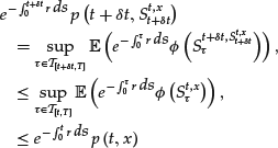
Our aim is now to show that the inequality in (19) is actually an equality. This is done in several steps, and requires us to identify an optimal stopping time ![]() for which the supremum in (15) is obtained. For a fixed (t, x), let us introduce the stopping time
for which the supremum in (15) is obtained. For a fixed (t, x), let us introduce the stopping time ![]() defined by
defined by
(notice that ![]() since
since ![]() ). It can be shown (see Appendix) that
). It can be shown (see Appendix) that
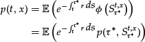
Using a decreasing property (65) proved in the Appendix, one then obtains that for any δ t>0,
This can be seen as a dynamic programming principle (or Bellman’s principle). For a European option we would have more simply
![]()
Now if we suppose that ![]() , then for any δ t>0 we have
, then for any δ t>0 we have ![]() . Considering Ito’s formula in (22), and by (17), we obtain
. Considering Ito’s formula in (22), and by (17), we obtain ![]() for
for ![]() , thus leading to
, thus leading to ![]() . This shows that the inequality in (19) is actually an equality.
. This shows that the inequality in (19) is actually an equality.
Hence the PDE for the American option is
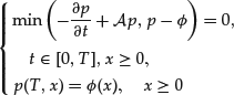
where ![]() is defined by (18). The major difference between the PDE (23) for American options and the PDE (8) for European options is that (23) is a nonlinear equation. This makes the theory of existence and uniqueness as well as the numerical approximation more difficult than for European options.
is defined by (18). The major difference between the PDE (23) for American options and the PDE (8) for European options is that (23) is a nonlinear equation. This makes the theory of existence and uniqueness as well as the numerical approximation more difficult than for European options.
In the presentation above, we have used Ito’s formula, which requires that p is C1 in time and C2 in the spot variable. This is not true in general. It is however possible, following the same lines, to prove that p is a weak solution to (23) in the viscosity sense. For a historical derivation of this PDE, see Bensoussan and Lions (1978) or El Karoui (1981) where a variational formulation of (23) is derived (see (52) below). We also refer to Oksendal and Rekvam (1998) for an infinite horizon-related problem, Crandall, Ishii, and Lions (1992) for general results, Pham (1998) for an approach of optimal stopping including jump diffusion processes, and to Barles (1994) for the case of a discontinuous payoff ![]() .
.
PRICING EUROPEAN OPTIONS WITH PDES
The aim of this section is to present two classes of methods for solving partial differential equations with some applications to the PDEs derived previously. We first introduce the finite difference method, which is based on approximation of the differential operators by Taylor expansions, and then the finite element methods, which belong to the wider class of Galerkin methods and are based on a variational formulation of the PDE. We try to stress the most important aspects of the numerical methods and refer, for example, to Achdou and Pironneau (2005 and 2009) for a more comprehensive presentation.
The Finite Difference Method for European Options
We first present the simplest approach to discretize a PDE: the finite difference method.
Basic Schemes
Let us introduce the finite difference method on the simple PDE (8). Let us first concentrate on the discretization of (8) with respect to the variable S. The principle is to divide the interval [0, Smax] into I intervals of length δ S = Smax/I (where Smax has to be chosen large enough, see below), and to approximate the derivatives by finite differences. A possible semidiscretization of (8) is: for ![]() ,
,
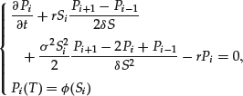
where Si = iδ S denotes the i-th discretization point, and Pi(t) is intended to be an approximation of p(t, Si). Now, (24) is a system of coupled ordinary differential equations (ODEs). The generalization to the case of a time and spot dependent r or σ is straightforward.
Notice that for S = 0, P0 can be solved independently (since S0 = 0): ![]() . In order to obtain a solution of the whole system of ODEs, one needs to define an appropriate boundary condition at S = Smax. Indeed, (24) taken at i = I involves PI+1 which is a priori not defined. There are basically two methods to deal with this issue. The first one consists of using some a priori knowledge on the values of p(t,S) when S is large and making some approximations of p(t, Smax). In this case, the value of PI is given as a data (this is a so-called Dirichlet boundary condition), and the unknowns are
. In order to obtain a solution of the whole system of ODEs, one needs to define an appropriate boundary condition at S = Smax. Indeed, (24) taken at i = I involves PI+1 which is a priori not defined. There are basically two methods to deal with this issue. The first one consists of using some a priori knowledge on the values of p(t,S) when S is large and making some approximations of p(t, Smax). In this case, the value of PI is given as a data (this is a so-called Dirichlet boundary condition), and the unknowns are ![]() . For example, in the case of a put (
. For example, in the case of a put (![]() ) (resp. a call (
) (resp. a call (![]() )), it is known that
)), it is known that ![]() (resp., in the limit
(resp., in the limit ![]() ,
, ![]() ), so that one can set PI(t) = 0 (resp.
), so that one can set PI(t) = 0 (resp. ![]() ). The error introduced by these artificial boundary conditions can be estimated. Another method is based on some knowledge on the asymptotic behavior of the derivatives of p. For example, in the case of the put, one can use the so-called homogeneous Neumann boundary condition, which writes
). The error introduced by these artificial boundary conditions can be estimated. Another method is based on some knowledge on the asymptotic behavior of the derivatives of p. For example, in the case of the put, one can use the so-called homogeneous Neumann boundary condition, which writes ![]() at the continuous level and
at the continuous level and ![]() at the discrete level. In this case, the unknowns are
at the discrete level. In this case, the unknowns are ![]() . For both methods, Smax should be chosen sufficiently large. In practice, the quality of the method may be assessed by measuring how sensitive the result is to the value of Smax.
. For both methods, Smax should be chosen sufficiently large. In practice, the quality of the method may be assessed by measuring how sensitive the result is to the value of Smax.
Let us now consider the time discretization. Here again, the idea is to divide the time interval [0, T] into N intervals of length δ t = T/N and to replace the time derivative by a finite difference. Three numerical methods are classically used:
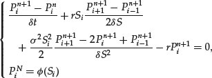
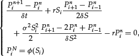
or

where Pni is intended to be an approximation of p(tn, Si), with tn = nδ t. Notice that using the discretization scheme (25) (the so-called explicit Euler scheme), the values of ![]() are explicitly obtained from the values of
are explicitly obtained from the values of ![]() . On the contrary, in the two other schemes (26) (implicit Euler scheme) or (27) (Crank-Nicolson scheme), the values of
. On the contrary, in the two other schemes (26) (implicit Euler scheme) or (27) (Crank-Nicolson scheme), the values of ![]() are obtained from the values of
are obtained from the values of ![]() through the resolution of a linear system, which is more demanding from the computational viewpoint. Various numerical methods can be used for solving this linear system; here, we cannot describe them in detail. Let us simply mention that basically, there exist two classes of methods: the direct methods, which are based on Gaussian elimination, and the iterative methods, which consist of computing the solution as the limit of a sequence of approximations and which only require matrix-vector multiplications. The method of choice depends on the characteristics of the problem.
through the resolution of a linear system, which is more demanding from the computational viewpoint. Various numerical methods can be used for solving this linear system; here, we cannot describe them in detail. Let us simply mention that basically, there exist two classes of methods: the direct methods, which are based on Gaussian elimination, and the iterative methods, which consist of computing the solution as the limit of a sequence of approximations and which only require matrix-vector multiplications. The method of choice depends on the characteristics of the problem.
Notions of Stability and Consistency
In order to analyze the convergence of the three discretization schemes (25), (26), and (27), and to understand the differences between these schemes, we need to introduce two important notions. The first notion is the consistency. A numerical method is said to be consistent if, when the exact solution is plugged into the numerical scheme, the error tends to zero when the discretization parameters tend to zero. In our context, it consists of replacing Pni in (25), (26), or (27) by p(tn, Si), where p satisfies (8), and to check that the remaining terms tend to zero when δt and δ S tend to zero. By using Taylor expansions, one can check that for (25) and (26) (resp. for (27)), the remaining terms are bounded from above by C(δ t+δ S2) (resp. by C(δ t2+δ S2)), where C denotes a constant, which depends on some norms of the derivatives of p. Therefore (25) and (26) (resp. (27)) are consistent discretization schemes of order 2 in the spot variable, and of order 1 (resp. 2) in time. The second important notion is the stability. A numerical method is said to be stable if the norm of the solution to the numerical scheme is bounded from above by a constant (independent of the discretization parameters) multiplied by the norm of the data (initial condition, boundary conditions, right-hand side). This property is clearly satisfied if the numerical method is convergent, that is, if the numerical approximation converges to the solution of the PDE when the discretization parameters tend to zero. A general result states that, conversely, a consistent and stable discretization scheme is indeed convergent. The estimate of convergence is given by the estimate of consistency error. For example, if p is smooth enough, the error for the EI scheme is bounded from above by C(δ t+δ S2). Notice that the constant C in these estimates depends on the solution p. Higher order schemes will lead to better error estimates as soon as the solution of the continuous problem is smooth enough: The higher the order, the more regular p must be in order to take full advantage of the scheme. For example, for some parameters, it may happen that the results obtained with the CN scheme around t = T are not better than those obtained with an order one scheme (IE or EE) since the solution is not sufficiently regular in time around t = T.
To give a precise meaning to all these results would require us to specify the norms used to measure the errors and to prove the stability. Let us simply mention that two norms are used in practice: The stability in ![]() -norm (the supremum of the absolute values of the components) is related to a discrete maximum principle (see below); and the stability in L2-norm (the Euclidean norm of the vector) is related to an energy estimate on the variational formulation. We refer, for example, to Achdou and Pironneau (2005) for more details.
-norm (the supremum of the absolute values of the components) is related to a discrete maximum principle (see below); and the stability in L2-norm (the Euclidean norm of the vector) is related to an energy estimate on the variational formulation. We refer, for example, to Achdou and Pironneau (2005) for more details.
The discrete maximum principle is the counterpart at the discrete level of the maximum principle at the continuous level mentioned above. It states that if the data for the numerical schemes are positive, then the solution is positive. Such schemes are by construction stable in ![]() -norm. There exist deterministic numerical methods based on a probabilistic representation of the stock evolution on a binomial or a trinomial tree. Such methods can be interpreted as explicit finite difference methods to solve the PDE (8) and naturally satisfy a discrete maximum principle.
-norm. There exist deterministic numerical methods based on a probabilistic representation of the stock evolution on a binomial or a trinomial tree. Such methods can be interpreted as explicit finite difference methods to solve the PDE (8) and naturally satisfy a discrete maximum principle.
Convergence Analysis
Let us now discuss the properties of the three discretization schemes. We already mentioned that they are all consistent. On the other hand, it can be shown that the explicit scheme (25) is stable under an additional assumption (a so-called CFL condition; see Courant, Friedrichs, and Lewy, 1967) of the form ![]() , where C denotes a positive constant. The other two schemes (26) and (27) are unconditionally stable (in L2-norm). In conclusion, with the explicit scheme, the values of
, where C denotes a positive constant. The other two schemes (26) and (27) are unconditionally stable (in L2-norm). In conclusion, with the explicit scheme, the values of ![]() can be very rapidly obtained from the values of
can be very rapidly obtained from the values of ![]() , but the time step must be sufficiently small with respect to the spot step to guarantee stability and hence convergence. On the other hand, the implicit schemes (26) and (27) require the resolution of a linear system at each time-step, but converge without any restriction on the time-step. This situation is very general for the parabolic PDEs obtained in finance. In terms of computational costs, the balance is generally in favor of the implicit schemes, since the CFL condition appears to be very stringent in practice. Concerning the stability in
, but the time step must be sufficiently small with respect to the spot step to guarantee stability and hence convergence. On the other hand, the implicit schemes (26) and (27) require the resolution of a linear system at each time-step, but converge without any restriction on the time-step. This situation is very general for the parabolic PDEs obtained in finance. In terms of computational costs, the balance is generally in favor of the implicit schemes, since the CFL condition appears to be very stringent in practice. Concerning the stability in ![]() -norm, let us just mention that the implicit schemes above do not satisfy the discrete maximum principle and are not
-norm, let us just mention that the implicit schemes above do not satisfy the discrete maximum principle and are not ![]() -stable as such. These properties are, however, satisfied after a small modification of the discretization of the advection term
-stable as such. These properties are, however, satisfied after a small modification of the discretization of the advection term ![]() (this is a so-called upwinding technique), which amounts to adding a diffusion term of order δ S, which implies that this modified scheme becomes only of order 1 in the spot variable. Thus, the price to pay to get
(this is a so-called upwinding technique), which amounts to adding a diffusion term of order δ S, which implies that this modified scheme becomes only of order 1 in the spot variable. Thus, the price to pay to get ![]() -stability is a loss of one order of convergence.
-stability is a loss of one order of convergence.
Table 1 Error on the Value of a Call in Function of the Number of Intervals I in the Variable S, for the Implicit Euler (IE) Scheme
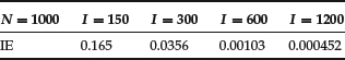
Table 2 Error on the Value of a Call in Function of the Number of Time-Steps N
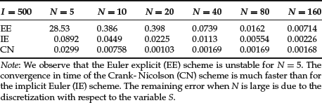
In Tables 1 and 2, we illustrate this analysis by computing the error on the price of a call with r = 0.1, σ = 0.01, K = 100, T = 1, S0 = 100, and Smax = 300 for the three discretization schemes (25), (26), and (27), and various values of the numerical parameters I and N. The reference value (P = 9.51625) is obtained by the analytic Black and Scholes formula. In particular, one can check that the rates of convergence with respect to δt and δ S are indeed those predicted by the analysis.
Before presenting an extension of this discretization method to Asian options, we mention the interest of a classical change of variable for the spot variable. It is indeed well known that by a change of variable x = ln S, it is possible to get rid of the dependency in S of the advection and diffusion terms in (8). It is not better to discretize the PDE after this change of variable, since it corresponds to taking a grid refined near S = 0, which is useless in this case. As we will see below, what actually matters is to refine the grid around the singularity of p (i.e., around S = K). A finite element approach is better suited in order to implement these refinements.
Application to Asian Options
We now present a less easy implementation of a finite difference method for pricing Asian options (see Dubois and Lelièvre, 2005). More precisely, we focus on computing numerical solutions to (14) for a fixed strike call:
(28) ![]()
We have seen in the previous section that a simple finite difference scheme leads to very satisfactory results when computing the solution of the classical Black-Scholes equation (8). On the other hand, when one uses a simple finite difference scheme on (14), very bad results are obtained, especially when the volatility σ is small (see Table 1 in Dubois and Lelièvre, 2005). These bad results are due to the fact that when ![]() is close to zero, the advection term
is close to zero, the advection term ![]() is much larger than the diffusion term
is much larger than the diffusion term ![]() in (14). This is known to deteriorate the stability of the numerical scheme, particularly with respect to the
in (14). This is known to deteriorate the stability of the numerical scheme, particularly with respect to the ![]() -norm. In practice, the numerical solution exhibits some oscillations and does not satisfy the discrete maximum principle. Moreover, the finite difference method introduces numerical diffusion, which leads to unsatisfactory results for purely advective equations.
-norm. In practice, the numerical solution exhibits some oscillations and does not satisfy the discrete maximum principle. Moreover, the finite difference method introduces numerical diffusion, which leads to unsatisfactory results for purely advective equations.
One way to handle this problem is to use a characteristic method (based on the solution of ![]() ) in order to get rid of the term 1/T. This means that the following change of variable is introduced:
) in order to get rid of the term 1/T. This means that the following change of variable is introduced:
(29) ![]()
One can easily show that g is solution of:1
The PDE (30) satisfied by g is such that when the advection term r(x−t/T) is small, the diffusion term ![]() is also small. As shown below, a finite difference scheme applied to (30) will indeed lead to satisfactory results.
is also small. As shown below, a finite difference scheme applied to (30) will indeed lead to satisfactory results.
An important property of the solution to (30) for ![]() is that (see Rogers and Shi, 1995)
is that (see Rogers and Shi, 1995) ![]() ,
,
and therefore, ![]() ,
,
To prove (31), one can notice that f given by (31) is the solution to (14) with ![]() , and that, due to the fact that the diffusion term is null for
, and that, due to the fact that the diffusion term is null for ![]() and that the advection term is negative, the solution to (14) for
and that the advection term is negative, the solution to (14) for ![]() on
on ![]() is the same as the solution to (14) for
is the same as the solution to (14) for ![]() on
on ![]() .
.
To discretize (30), a Crank-Nicolson time scheme is used, with a uniform time step δ t = T/N. In order to use the fact that g is analytically known on ![]() (see (32)), a mesh that properly discretizes the boundary x = t/T is used. Therefore, the space interval (0, 1) is also discretized with N space steps of length δ x = 1/N (see Figure 1). The mesh is completed by adding J intervals on the right-hand side of x = 1, so that
(see (32)), a mesh that properly discretizes the boundary x = t/T is used. Therefore, the space interval (0, 1) is also discretized with N space steps of length δ x = 1/N (see Figure 1). The mesh is completed by adding J intervals on the right-hand side of x = 1, so that ![]() with
with ![]() . The value J = N/2 has been found to be sufficient to guarantee the independence of the results on the position of xmax.
. The value J = N/2 has been found to be sufficient to guarantee the independence of the results on the position of xmax.
Figure 1 The Mesh and the Computational Domain for the Finite Difference Scheme Used to Discretize (30)
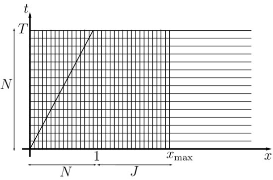
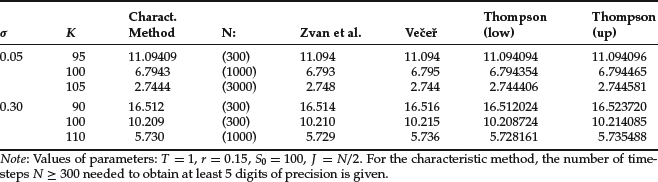
Table 3 Comparisons of the Prices for an Asian Fixed Call Obtained with Various Finite Difference Methods: Characteristic Method, Zvan et al. (1998), Večeř (2001), and Thompson (1999)
Notice that at time tn = nδ t, the number of unknowns is (N+J−n). This means that the dimension of the linear system to solve depends on the time-step.
As far as boundary conditions are concerned, we use a Dirichlet boundary condition on x = t/T (using (32)) and an artificial zero Neumann boundary condition on ![]() .
.
Let us now give some numerical results. In Table 3, a few comparisons of the results obtained with the characteristic method and other methods are given. The characteristic method appears to be accurate for both small and large volatilities. For any values of the parameters, at least 5 digits of precision are obtained in less than one second. Notice that the Thompson bounds and the characteristic method are implemented in Premia.2
The Finite Element Method for European Options
We would like now to introduce the finite element method. This technique is more flexible than the finite difference method. In particular, it allows for local refinements of the spot grid (even in dimensions greater than one), and possibly based on local error estimators that are mentioned below. This is particularly important for American options, because the pricing function is singular near the exercise boundary, and this curve is not known a priori. Let us emphasize that the use of a refined mesh around the singularities of the solution (for example, for vanilla option pricing problems, around t = T and S = K) is very important in practice to rapidly obtain accurate results. The finite element method can also be used in a flexible way when the geometry of the computational domain becomes complex, which may be of interest for barrier options in dimensions greater than one. Finally, finite element methods are interesting since they are naturally stable (in L2-norm) and optimal error bounds (in L2-norm) can be derived.
In the following, we first present the finite element method on a simple example, namely equation (8). We then show how to treat more complex European options.
Variational Formulation and Finite Element Space
The conforming finite element method is based on two ingredients: a so-called variational formulation of the PDE on a functional space V and the choice of an appropriate sequence of finite dimensional spaces ![]() , which tends to V when h (which is the typical diameter of the cells of the space mesh) tends to 0. Let us illustrate this on (8).
, which tends to V when h (which is the typical diameter of the cells of the space mesh) tends to 0. Let us illustrate this on (8).
To derive a variational formulation of (8), the principle is to multiply the equation by a test function of the spot variable and to integrate by parts. For these computations to be well defined, the functions need to be sufficiently smooth. We thus introduce the functional spaces ![]() , and
, and ![]() . Assuming that
. Assuming that ![]() is square integrable, a variational formulation of (8) is then (for an S-dependent volatility σ): Find
is square integrable, a variational formulation of (8) is then (for an S-dependent volatility σ): Find ![]() such that for all
such that for all ![]() ,
,
All the integrals are with respect to ![]() . This rewrites: Find
. This rewrites: Find ![]() such that for all
such that for all ![]() ,
,
where a is the bilinear form
Under suitable assumptions on the data (r, σ, and ![]() ), it is possible to prove that this variational problem is well posed (see Achdou and Pironneau, 2005).
), it is possible to prove that this variational problem is well posed (see Achdou and Pironneau, 2005).
The second step is to introduce a sequence of meshes in the spot variable indexed by the maximal step h and related finite dimensional functional spaces ![]() . In the case of (33), the problem is posed on an infinite domain, and one needs to first localize the PDE in a finite domain [0, Smax] by using artificial boundary condition at S = Smax, as already explained for finite difference discretizations. We consider, for example, a zero Neumann boundary condition on S = Smax:
. In the case of (33), the problem is posed on an infinite domain, and one needs to first localize the PDE in a finite domain [0, Smax] by using artificial boundary condition at S = Smax, as already explained for finite difference discretizations. We consider, for example, a zero Neumann boundary condition on S = Smax: ![]() . Then, a mesh of [0, Smax] consists of a finite number of intervals (Si, Si+1) with S0 = 0 and SI = Smax. We set
. Then, a mesh of [0, Smax] consists of a finite number of intervals (Si, Si+1) with S0 = 0 and SI = Smax. We set ![]() . The intervals (Si, Si+1) are called elements. We then need to define a functional space Vh associated with the mesh. A classical example is the P1 finite element space, which contains continuous and piecewise affine functions, namely, continuous functions, which are affine on each interval (Si, Si+1), for
. The intervals (Si, Si+1) are called elements. We then need to define a functional space Vh associated with the mesh. A classical example is the P1 finite element space, which contains continuous and piecewise affine functions, namely, continuous functions, which are affine on each interval (Si, Si+1), for ![]() . In this case, a basis of the vector space Vh is given by the so-called hat functions
. In this case, a basis of the vector space Vh is given by the so-called hat functions ![]() such that for
such that for ![]() ,
, ![]() is the Kronecker symbol). Notice that higher order finite element methods may be easily obtained by taking continuous and element-wise polynomial functions of degree k>1.
is the Kronecker symbol). Notice that higher order finite element methods may be easily obtained by taking continuous and element-wise polynomial functions of degree k>1.
The discretization in the spot price variable now simply consists in replacing the functional space V by the finite dimensional space Vh in (33) or (34) (this is the principle of Galerkin methods): Find ![]() such that for all
such that for all ![]() ,
,
where ![]() is an approximation of
is an approximation of ![]() in the space Vh, and where the integrals in the bilinear form a are here for
in the space Vh, and where the integrals in the bilinear form a are here for ![]() (see (35)). One can take, for example,
(see (35)). One can take, for example, ![]() such that
such that ![]() for all
for all ![]() (
(![]() is then the L2 projection of
is then the L2 projection of ![]() onto Vh). Problem (36) is a finite-dimensional problem in space of the form
onto Vh). Problem (36) is a finite-dimensional problem in space of the form ![]() , where Ph(t) is a vector of dimension I containing the values of ph at the nodes of the mesh (
, where Ph(t) is a vector of dimension I containing the values of ph at the nodes of the mesh (![]() ) and Mh, Ah are
) and Mh, Ah are ![]() matrices. The matrix Mh (resp. Ah), with (i, j)-th component
matrices. The matrix Mh (resp. Ah), with (i, j)-th component ![]() (resp. a(qj, qi)) is classically called the mass (resp. stiffness) matrix, because the finite element method was originally popularized by the mechanical engineering community. When using the nodal basis (hat functions), these matrices are very sparse (tridiagonal for one-dimensional problems). Problem (36) is somewhat similar to (24) obtained by the finite difference method; the two problems (24) and (36) are actually equivalent if a mesh with uniform space steps is used, and if Mh is replaced by a close diagonal matrix (mass-lumping).
(resp. a(qj, qi)) is classically called the mass (resp. stiffness) matrix, because the finite element method was originally popularized by the mechanical engineering community. When using the nodal basis (hat functions), these matrices are very sparse (tridiagonal for one-dimensional problems). Problem (36) is somewhat similar to (24) obtained by the finite difference method; the two problems (24) and (36) are actually equivalent if a mesh with uniform space steps is used, and if Mh is replaced by a close diagonal matrix (mass-lumping).
A fundamental result (the Cea’s lemma) states that the norm of (p−ph) (the discretization error) is bounded from above by a constant times the infimum of the norm of (p−qh), over all ![]() (the best fit error). Using this result, if Vh gets closer to V when h tends to 0, that is, if the best fit error tends to 0 when h tends to zero, so does the discretization error. In particular, the finite element discretization is thus naturally stable in this norm. A precise meaning for this statement requires us to define the norm and study the best fit error. Let us simply mention that the norms used in this context are related to the L2-norm introduced for finite difference schemes. We refer to Achdou and Pironneau (2005) or Quarteroni and Valli (1997) for the details. In our specific example, it is possible to prove that, if the payoff function is regular enough, then
(the best fit error). Using this result, if Vh gets closer to V when h tends to 0, that is, if the best fit error tends to 0 when h tends to zero, so does the discretization error. In particular, the finite element discretization is thus naturally stable in this norm. A precise meaning for this statement requires us to define the norm and study the best fit error. Let us simply mention that the norms used in this context are related to the L2-norm introduced for finite difference schemes. We refer to Achdou and Pironneau (2005) or Quarteroni and Valli (1997) for the details. In our specific example, it is possible to prove that, if the payoff function is regular enough, then
![]()
and that
![]()
For the discretization in time, the situation is exactly the same as for the finite difference method: One can use the explicit Euler scheme, implicit Euler scheme, or Crank-Nicolson scheme, and the rate of convergence is O(δ t) for the Euler schemes and O(δ t2) for the Crank-Nicolson scheme.
Finite Element Methods for Other Options
We have introduced the finite element method in a very simple case. The aim of this section is to explain how it applies for other options.
Let us first consider basket options, or basket options with barriers, in dimension 2 and 3. The derivation of a variational formulation for (9) is very similar to the one-dimensional case. However, the construction of the mesh is much more complicated in dimension 2 and 3, than in dimension 1. It consists of partitioning the domain into non-overlapping cells (elements) whose shapes are simple and fixed (for example, triangles or quadrilaterals in dimension 2, or tetrahedra or hexahedra in dimension 3). The functional spaces Vh can then be constructed as in dimension 1, for example, by considering continuous piecewise affine functions. One interest of the finite element method in this context is that it is possible to mesh any domain ![]() for barrier options. In the finite difference method, to mesh nonquadrilateral (or nonhexahedral) domains is complicated.
for barrier options. In the finite difference method, to mesh nonquadrilateral (or nonhexahedral) domains is complicated.
Let us now consider the case of lookback options whose prices satisfy (11). This is a natural variational formulation of (11) (written here for a constant volatility σ): Find ![]() such that, for all
such that, for all ![]() ,
,
(37) 
where ![]() . The boundary condition
. The boundary condition ![]() is naturally contained in this variational formulation since, by integration by parts over
is naturally contained in this variational formulation since, by integration by parts over ![]() :
:
The first term corresponds to the diffusion term in (11). The second term is an integral over the boundary ![]() of
of ![]() and naturally enforces the boundary condition
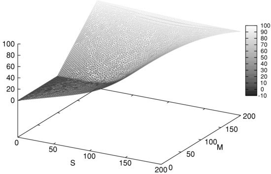
and naturally enforces the boundary condition ![]() . In Figure 2, we represent the price of a fixed strike call obtained using the formulation (11), an implicit Euler scheme, and P1 finite elements. The computations are made with FreeFem++.3
. In Figure 2, we represent the price of a fixed strike call obtained using the formulation (11), an implicit Euler scheme, and P1 finite elements. The computations are made with FreeFem++.3
Figure 2 Price of a Lookback Option for a Fixed Strike Call: ![]()
Note: The parameters are: σ = 0.3, r = 0.1, K = 100, T = 1.
A Posteriori Error Estimates
A frequently mentioned advantage of the Monte Carlo methods is that they naturally provide a posteriori error bounds through a confidence interval, typically built upon the central limit theorem. It is also possible to obtain such a posteriori error estimates in the framework of the finite element method (this is one additional advantage of this method compared to finite difference methods). Moreover, these a posteriori estimates have two very important features:
- They depend on local error indicators.
- They can be proved to be reliable and efficient, that is, the actual error is bounded above and below by some fixed constants times the a posteriori error, and these estimates can be made local.
Therefore, in the finite element method, the a posteriori error estimates enable us to refine the mesh in space and time adaptively. We will give a numerical illustration for American options and refer to Ern, Villeneuve, and Zanette (2004), Achdou and Pironneau (2005 and 2009), or Achdou, Hecht, and Pommier (2008) for more details.
High-Dimensional Problems
In practical problems, options often involve more than three assets. In this case, the PDE is posed in a space of dimension larger than 4, and the finite element or difference methods cannot be used, since the number of unknowns typically grows exponentially with respect to the problem’s dimension. This is the so-called curse of dimensionality. Let us mention that such high-dimensional problems also appear in other scientific fields, quantum chemistry, for example, and that it is still a subject of current research to build appropriate discretizations for high-dimensional PDEs. Roughly speaking, the problem is to find an appropriate sequence of functional spaces Vh (whose basis is called a Galerkin basis), such that their dimensions do not grow too rapidly with the dimension of the problem. One approach is the sparse tensor product (see Bungartz and Griebel, 2004; Petersdoff and Schwab, 2004). The main difficulty when using this approach is actually to project the initial condition on Vh. Another approach used in other contexts for solving high-dimensional problems by deterministic methods is the low separation rank method (see Beylkin and Mohlenkamp, 2002) and the related greedy algorithms (see Ammar et al., 2002; Temlyakov, 2008; Le Bris, Lelièvre, and Maday, 2009; and Nouy, 2009). Let us finally mention that another possible approach for building an appropriate Galerkin basis would be the reduced basis method, where some solutions for a given set of parameters are used to approximate the solution for other values of the parameters. Such methods are currently actively investigated (see, for example, Boyaval, Le Bris, Lelièvre, Maday, Nguyen, and Patera, 2010).
The Uncertain Volatility Model: An Example of a Nonlinear PDE
One major interest of the PDE approach is that it can be applied for nonlinear models. This will be the case for American options, see below, but we would like to give here another example of such a situation. The principle of the uncertain volatility model introduced by Avellaneda, Levy, and Paras (1995) is to give a price for a European option, when the volatility is only supposed to be in an interval [σ min, σ max]. The principle is the following. For a European option with convex payoff, it is easy to check that the price should be the Black-Scholes price obtained with the maximum volatility σ max. In this case, the profit and loss for the hedging strategy is indeed zero if the realized volatility is constant equal to σ max. A similar reasoning holds for concave payoffs: In this case, one should consider the Black-Scholes price with the minimum volatility σ min. For a general payoff, it is thus natural (and it can be checked that this is indeed an approach that leads to a very good hedging strategy, with small profit and loss, and thus cheap price) to consider the solution p to the PDE:
(38) 
In other words, σ max (resp. σ min) is used where the price is convex (resp. concave), as a function of the spot. This PDE can be solved using extensions of the discretization techniques presented above; see, for instance, section 2.4 in van der Pijl and Oosterlee (2011).
PRICING AMERICAN OPTIONS WITH PDES
This section is devoted to the discretization of the system (23) for the price of an American option. Notice that no closed formulas such as the Black-Scholes formula are available for American put, or for American call with a dividend rate, so that efficient discretization of this system is needed even for these simple payoffs.
The Finite Difference Approach for American Options
We first present the extension of the finite difference approach presented above for European options to American options.
Some Finite Difference Schemes
We consider a regular mesh discretization Si = iδ S and a time discretization tn = nδ t with ![]() . As in the European case, it is natural to consider the following three iterative numerical schemes for Pni, an approximation of p(tn, Si). In all cases, the scheme is initialized by
. As in the European case, it is natural to consider the following three iterative numerical schemes for Pni, an approximation of p(tn, Si). In all cases, the scheme is initialized by ![]() . Let A be the matrix such that
. Let A be the matrix such that
(39) 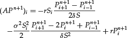
The explicit Euler (EE) scheme for (23) is, for ![]() ,
,
The scheme computes ![]() from the knowledge of
from the knowledge of ![]() . Similarly, we can propose an implicit Euler (IE) scheme:
. Similarly, we can propose an implicit Euler (IE) scheme:
and an (implicit) Crank-Nicolson (CN) scheme
In the case of the EE scheme, it is easy to see that we have the equivalent formulation
where Id denotes the identity matrix.
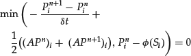
We now have two new difficulties compared to the European case: First, the well-posedness of the schemes (41) or (42) is not immediate (for European options, we obtained a linear system, but this is no longer true for American options), and second, studying the convergence is more difficult.
One way to circumvent the first difficulty is to introduce a splitting method (see Barles and Souganidis, 1991; Barles, Daher, and Romano, 1995; and Lions and Mercier, 1979). For (23), it writes (a similar modification of (42) could also be considered, yielding a Crank Nicolson-splitting (CN-S) scheme):
(44b) ![]()
Hereafter, (44) will be refered to as the implicit Euler-splitting (IE-S) scheme. The first step (44a) consists of solving a linear system, as in the European case. The second step is a projection on the set ![]() , as for the EE scheme (43).
, as for the EE scheme (43).
Notice that as for European options, we set the equation on a truncated domain (0, Smax) and use artificial boundary conditions on S = Smax. We refer to Barles, Daher, and Romano (1995) for error estimates between the truncated problem on (0, Smax) and the exact problem.
An Abstract Convergence Result
Assuming for the moment that the schemes are well posed, it is possible to study the convergence in the general framework of finite different schemes for Hamilton-Jacobi equations. Possibly under some restrictions on the mesh sizes δt and δ S, we can obtain convergence to the viscosity solution of the PDE (23). We refer to Barles (1994) or Barles, Daher, and Romano (1995) for a short introduction, and Crandall, Ishii, and Lions (1992) for a more detailed overview. To give a rough idea of the convergence results for such schemes, we consider a general Hamilton-Jacobi equation of the form
with a terminal condition on ![]() , where H is assumed to be Lipschitz continuous and “backward parabolic” in the sense that
, where H is assumed to be Lipschitz continuous and “backward parabolic” in the sense that
(46b) ![]()
Equation (23) is indeed of the form of (45) with, for ![]() ,
, ![]() , which obviously satisfies (46).
, which obviously satisfies (46).
First convergence results were given in the fundamental work of Crandall and Lions (1984) for Lipschitz continuous final condition ![]() (and without
(and without ![]() dependence in (45)).
dependence in (45)).
An abstract and general convergence result is given by Barles and Souganidis (1991), and we now give a simplified presentation of this result.
We first assume that H satisfies a comparison principle, which can be seen as an extension of the maximum principle to some nonlinear equations. The comparison principle is roughly the following (see Crandall, Ishii, and Lions, 1992; Barles, 1994; or Pham, 1998): Assume that u (resp. v) is a subsolution (resp. supersolution) of (45), that is,
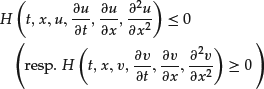
for ![]() , and that
, and that ![]() on the boundaries S = Smax and t = T, then
on the boundaries S = Smax and t = T, then ![]() everywhere.
everywhere.
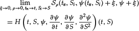
Now, suppose that we can write the scheme in the abstract form: ![]() ,
, ![]() ,
,
where ![]() , and [P] stands for a continuous function that takes values
, and [P] stands for a continuous function that takes values ![]() on the corresponding grid points (tk, Sj).4 We suppose that (47) admits at least one solution denoted
on the corresponding grid points (tk, Sj).4 We suppose that (47) admits at least one solution denoted ![]() . Then, in the limit when ρ goes to zero,
. Then, in the limit when ρ goes to zero, ![]() converges to p solution to (45) if the following conditions are satisfied:
converges to p solution to (45) if the following conditions are satisfied:
For a weaker statement see Barles and Souganidis (1991).
![]()
For most standard financial options, a comparison principle holds. The stability and consistency conditions are close to the stability and consistency conditions already introduced in the case of the schemes for European options. Hence the new condition to check is the monotonicity assumption (which is related to the property (46a) satisfied by H). It is actually related to a discrete maximum principle.
Error estimates can also be obtained for the finite difference schemes (40)–(41)–(42). For example, for the EE scheme, an error estimate of order δ S1/2 in ![]() -norm can be proved under a CFL condition and for Lipschitz initial data (see Jackobsen, 2003). In the context of the finite element method (see below) an error estimate of order δ S2 can be proved, but in the weaker L2-norm.
-norm can be proved under a CFL condition and for Lipschitz initial data (see Jackobsen, 2003). In the context of the finite element method (see below) an error estimate of order δ S2 can be proved, but in the weaker L2-norm.
Implementation and Convergence of the Finite Difference Schemes
It is easy to see, in view of (43), that the EE scheme is stable and monotone if the components of the matrix (Id−δ tA) are nonnegative. This is exactly what is needed to prove a discrete maximum principle in the European case. This property holds under a CFL condition of the form ![]() , C constant, and with an appropriate discretization of the advection term. The CN scheme is also stable and monotone under a CFL-like condition. On the other hand, it can be shown that the IE-S scheme as well as the IE scheme are stable and monotone without any CFL condition.
, C constant, and with an appropriate discretization of the advection term. The CN scheme is also stable and monotone under a CFL-like condition. On the other hand, it can be shown that the IE-S scheme as well as the IE scheme are stable and monotone without any CFL condition.
Now let us explain how to solve the implicit schemes (41) or (42) in practice. Let us consider the IE scheme (41). At each time step, setting b = Pn+1, B = Id+δ tA and ![]() , the problem is equivalent to finding x = Pn such that
, the problem is equivalent to finding x = Pn such that
The Howard algorithm (see Howard, 1960; also called the policy iteration algorithm) is the method of choice to solve (48). To present this algorithm, we rewrite (48) in the following form: Find x such that,
where ![]() (where δ i,j is again the Kronecker symbol, i.e., the (i, j)-th component of Id) and
(where δ i,j is again the Kronecker symbol, i.e., the (i, j)-th component of Id) and ![]() . The i-th component of
. The i-th component of ![]() only depends on the i-th component of α, so that the minimum for the i-th component in (49) is indeed taken with respect to the i-th component of α. Thus, for a given x and α realizing the minimum in (49), the component
only depends on the i-th component of α, so that the minimum for the i-th component in (49) is indeed taken with respect to the i-th component of α. Thus, for a given x and α realizing the minimum in (49), the component ![]() is equal to 0 (resp. to 1) if, at the i-th node, the minimum in (48) is (Bx−b)i (resp. (x−g)i). For an initial value5
is equal to 0 (resp. to 1) if, at the i-th node, the minimum in (48) is (Bx−b)i (resp. (x−g)i). For an initial value5 ![]() , the algorithm is written as follows: Iterate for
, the algorithm is written as follows: Iterate for ![]() ,
,
Santos and Rust (2004) and Bokanowski, Maroso, and Zidani (2009) provide some convergence results. Under suitable assumptions on the matrix B (which are satisfied for the schemes considered above, which satisfy the monotonicity condition), it can be proved that this method converges in at most I iterations. In practice, only a few iterations are needed for solving (41).
This algorithm can also be seen as:
- A Newton’s method on the function F defined by Fi(x) = min((Bx−b)i, (x−g)i). More precisely, it is a semismooth Newton’s method applied to the slantly differentiable function6 F.
- A primal-dual algorithm to implement the fully implicit Euler scheme (41) as introduced in Hintermüller, Ito, and Kunisch (2002).
Another well-known method for solving (48) is the projected successive over relaxation (PSOR) method, which is a modification of the successive over relaxation (SOR) method to solve iteratively systems of linear equations (see Saad, 2003). In its simplest form, it consists of decomposing B = L+U where L is a lower triangular matrix and U is an upper triangular matrix with zero coefficients on the diagonal. The algorithm consists of choosing an initial guess x0 and then computing iteratively for ![]() , for
, for ![]() ,
, ![]() . This method converges only if B is a diagonal dominant matrix, and the convergence is rather slow in practice. However, it leads to a highly efficient method for the finite element method discussed below, when combined with a suitable splitting scheme.
. This method converges only if B is a diagonal dominant matrix, and the convergence is rather slow in practice. However, it leads to a highly efficient method for the finite element method discussed below, when combined with a suitable splitting scheme.
For the specific case of an American put option on a single asset, a fast algorithm was proposed by Brennan and Schwartz (1977) for solving (41) and proved to converge in Jaillet, Lamberton, and Lapeyre (1990) in the finite element setting (see also Bokanowski, Maroso, and Zidani [2009] in the finite difference setting). Also in this case it can be proved that the region of exercise (namely ![]() ) is of the form
) is of the form ![]() where
where ![]() is continuous under some regularity assumption of the data. Then the Howard algorithm takes a simple form, which is known as the front-tracking algorithm (see, for instance, Achdou and Pironneau, 2005). However, these algorithms are very specific to the one-dimensional case and do not apply for general payoff functions.
is continuous under some regularity assumption of the data. Then the Howard algorithm takes a simple form, which is known as the front-tracking algorithm (see, for instance, Achdou and Pironneau, 2005). However, these algorithms are very specific to the one-dimensional case and do not apply for general payoff functions.
Numerical Results for the American Put Option
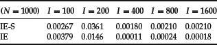
In Table 4, we give numerical results obtained with the IE-S and IE schemes for an American put option with r = 0.1, σ = 0.1, K = 100, T = 1, S = 100, and Smax = 150. We have computed all error values by taking the reference value P = 1.63380 (obtained with a Cox-Ross-Rubinstein algorithm with N = 105, CPU-time = 1750 s.; see Cox, Ross, and Rubinstein [1979] and Lamberton and Lapeyre [1997]). In this example, the IE scheme is one digit more accurate than the IE-S scheme. With these numerical parameters, the EE scheme would yield bad results since the CFL condition is not respected. The IE scheme has been implemented using the Howard algorithm. The remaining error when I is large is due to the time discretization.
Table 4 Error on the Value of an American Put in Function of the Number I of Intervals in the Variable S (and for N = 1000)
In Table 5, we compare the EE, IE-S and IE schemes. Since the error is of order of O(δ t)+O(δ S2), we have used parameters N and I such that ![]() (i.e.,
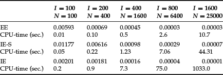
(i.e., ![]() ), and such that the CFL condition is satisfied. We remark that the EE scheme gives satisfactory results in less than a few seconds. The IE is more accurate but more costly than IE-S. Hence in view of the CPU-time it is more advantageous here to use simply the EE or the IE-S scheme. This conclusion holds for a finite difference discretization, but may be different for a finite element discretization, or for another set of parameters.
), and such that the CFL condition is satisfied. We remark that the EE scheme gives satisfactory results in less than a few seconds. The IE is more accurate but more costly than IE-S. Hence in view of the CPU-time it is more advantageous here to use simply the EE or the IE-S scheme. This conclusion holds for a finite difference discretization, but may be different for a finite element discretization, or for another set of parameters.
Table 5 Error and CPU-Times for the Value of an American Put as a Function of the Number N of Time-Steps N and the Number I of Intervals in the Variable S
Markov Chains Approximations
There exist related discretization schemes for American options based on Markov chain approximations. Markov chain schemes (see Kushner and Dupuis, 2001) are based on the approximation of the dynamic programming principle between times t and t+δ t and on the use of a spatial interpolation over a mesh (Sj). This leads to another class of schemes that are also in finite difference form. Their convergence can be established by showing the convergence to the dynamic programming equation, or by using the Barles-Souganidis theorem (see Barles and Souganidis, 1991). Finite difference schemes enter this framework as well as semi-Lagrangian schemes (Capuzzo-Dolcetta and Falcone, 1989; Falcone and Ferretti, 1994). An inversed CFL condition, typically of the form ![]() can then be needed. Notice that the Cox-Ross-Rubinstein algorithm (Cox, Ross, and Rubinstein, 1979) can also be seen as a discrete Markov chain approximation scheme using a very particular spatial mesh such that no interpolation appears at the end.
can then be needed. Notice that the Cox-Ross-Rubinstein algorithm (Cox, Ross, and Rubinstein, 1979) can also be seen as a discrete Markov chain approximation scheme using a very particular spatial mesh such that no interpolation appears at the end.
Portfolio Optimization
The techniques developed above for pricing American options can be used in the context of portfolio optimization. A portfolio optimization problem (or stochastic optimization problem) is typically of the form
where K is compact, α is a progressively measurable function with values in K, and with
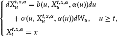
The corresponding PDE can be shown to be
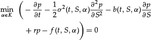
in the viscosity sense (see Pham, 2006). Finite difference schemes similar to those presented above for American options can be applied. Implicit schemes, if considered, can be solved by the Howard algorithm. This can also be generalized to an optimal stopping time problem, adding in (50) a supremum over stopping times with values in [t, T] (as in (15)). For such general HJB equations, a discretization by a finite element approach is not always possible because an appropriate variational formulation cannot always be obtained; see Bensoussan and Lions (1978).
The Finite Element Approach for American Options
As in the European case, the finite element approach requires a variational formulation of the PDE (23). Let us consider the case of the American put option. Let V be the functional space used for the variational formulation, and
![]()
We first notice that (23) is equivalent to the set of inequalities7
(together with ![]() )
)
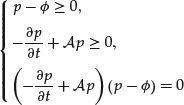
We can check that this is equivalent (for sufficiently smooth function p) to the following variational formulation for (23): find ![]() such that for all
such that for all ![]() ,
,
where a is the bilinear form (35) defined above (recall that for compactly supported functions p and q, ![]() ), with the final condition
), with the final condition
![]()
Indeed, by writing ![]() , it is clear that (51) implies (52). Conversely, choosing a sufficiently large
, it is clear that (51) implies (52). Conversely, choosing a sufficiently large ![]() in (52), we obtain that
in (52), we obtain that ![]() . Taking then
. Taking then ![]() in (52), we obtain that
in (52), we obtain that ![]() , but this inequality is actually an equality since
, but this inequality is actually an equality since ![]() and
and ![]() .
.
Notice that if we take K = V in (52), we recover the variational formulation (34) for the European option. Precise existence and uniqueness results for such variational inequalities can be found in Bensoussan and Lions (1978). For results and applications in the finance context, we refer to Achdou and Pironneau (2005 and 2009).
Now, as in the case of the finite element method for European options, we introduce a sequence of finite dimensional functional spaces ![]() , such that the functions in V are better and better approximated by functions in Vh as h goes to 0. One can, for example, consider a P1 finite element space on a mesh
, such that the functions in V are better and better approximated by functions in Vh as h goes to 0. One can, for example, consider a P1 finite element space on a mesh ![]() . Remember that a basis of Vh is given by a set of functions
. Remember that a basis of Vh is given by a set of functions ![]() . The finite element approximation of (52) is obtained by replacing V by Vh: Find
. The finite element approximation of (52) is obtained by replacing V by Vh: Find ![]() such that for all
such that for all ![]() ,
,
with the final condition ![]() , where
, where ![]() is an approximation of
is an approximation of ![]() .
.
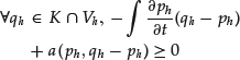
For time discretization, one can again use the schemes we have introduced in the case of the discretization of European options. For example, the implicit Euler scheme applied to (53) is naturally defined as follows: Find ![]() in
in ![]() such that
such that ![]() (initialization) and, for
(initialization) and, for ![]() :
:
One can easily check that
![]()
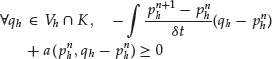
Denoting Ah and Mh the mass and stiffness matrices as in the case of the finite element method for European options, and reasoning as for the equivalence between (23), (51), and (52), it can be checked that (54) is equivalent to solve in ![]() :
:
Figure 3 The Adapted Mesh and the Contours of P One Year to Maturity. σ 1 = 0.2, σ 2 = 0.1, ![]() .
.
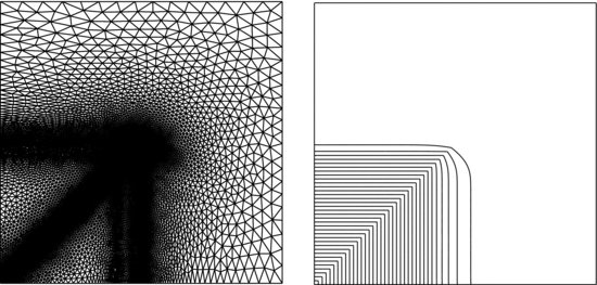
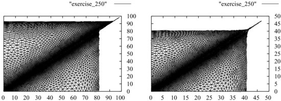
Figure 4 The Exercise Region One Year to Maturity. Left: K = 100, σ 1 = 0.2, σ 2 = 0.1, ![]() . Right: K = 50, σ 1 = σ 2 = 0.2,
. Right: K = 50, σ 1 = σ 2 = 0.2, ![]() .
.
where ![]() and Pni = pnh(Si). Equivalently, the problem is to find Pn such that
and Pni = pnh(Si). Equivalently, the problem is to find Pn such that
![]()
This is a similar problem as for the IE finite difference scheme (see (48)) where the matrix (Id+δ tA) is now replaced by (Mh+δ tAh). It can be solved by the Howard algorithm previously presented. For the particular American put problem under some assumptions on the mesh steps δt and h, it can also be solved by the Brennan and Schwartz algorithm or the front-tracking algorithm mentioned above.
Notice that a Crank-Nicolson scheme can be derived in a similar way. The expected error (in L2-norm) is (as in the European case) O(h2)+O(δ t) for the IE scheme and O(h2)+O(δ t2) for the CN scheme.
We conclude this section by a numerical illustration of the mesh refinement procedure (that can be implemented by using a posteriori error estimates) applied to the pricing of an American option on two assets. Such an automatic refinement procedure is particularly useful for American options because the pricing function is not smooth at any given time ![]() . Figures 3 and 4 illustrate such a mesh refinement for a typical two-assets American option with payoff
. Figures 3 and 4 illustrate such a mesh refinement for a typical two-assets American option with payoff ![]() . The artificial boundary
. The artificial boundary ![]() is
is ![]() . Homogeneous Dirichlet conditions are imposed on
. Homogeneous Dirichlet conditions are imposed on ![]() . We have chosen two examples. In the first example, the parameters are σ 1 = 0.2, σ 2 = 0.1, r = 0.05,
. We have chosen two examples. In the first example, the parameters are σ 1 = 0.2, σ 2 = 0.1, r = 0.05, ![]() , and K = 100. In the second example, the parameters are σ 1 = σ 2 = 0.2, r = 0.05,
, and K = 100. In the second example, the parameters are σ 1 = σ 2 = 0.2, r = 0.05, ![]() , and K = 50. The implicit Euler scheme has been used with a uniform time step of 1/250 year. For the variables S1 and S2, we have used adaptive finite elements. For solving the linear complementarity problems, we have used the Howard algorithm. Mesh adaption in the (S1, S2) variable has been performed every 1/10 year. In Figure 3, we have plotted the adapted mesh (left) and the contours of the pricing function (right) one year to maturity for the first example. Note that the contours exhibit right angles in the exercise region. In Figure 4, we plot the exercise region one year to maturity for the first example (left) and for the second example (right). One sees that the exercise boundary has singularities. It is also visible that the mesh has been adapted near the exercise boundary.
, and K = 50. The implicit Euler scheme has been used with a uniform time step of 1/250 year. For the variables S1 and S2, we have used adaptive finite elements. For solving the linear complementarity problems, we have used the Howard algorithm. Mesh adaption in the (S1, S2) variable has been performed every 1/10 year. In Figure 3, we have plotted the adapted mesh (left) and the contours of the pricing function (right) one year to maturity for the first example. Note that the contours exhibit right angles in the exercise region. In Figure 4, we plot the exercise region one year to maturity for the first example (left) and for the second example (right). One sees that the exercise boundary has singularities. It is also visible that the mesh has been adapted near the exercise boundary.
CALIBRATION
Let us now discuss the question of the determination of the parameters that appear in the models we introduced, with an emphasis on the calibration of the local volatility.
Limitation of the Black-Scholes Model: The Need for Calibration
Consider a European-style option on a given stock with a maturity T and a payoff function ![]() , and assume that this option is on the market. Call p its present price. Also, assume the risk-free interest rate is the constant r. One may associate with p the so-called implied volatility, that is, the volatility σ imp such that the price given by formula (4) at time t = 0 with σ = σ imp coincides with p. If the Black-Scholes model was sharp, then the implied volatility would not depend on the payoff function
, and assume that this option is on the market. Call p its present price. Also, assume the risk-free interest rate is the constant r. One may associate with p the so-called implied volatility, that is, the volatility σ imp such that the price given by formula (4) at time t = 0 with σ = σ imp coincides with p. If the Black-Scholes model was sharp, then the implied volatility would not depend on the payoff function ![]() . Unfortunately, for vanilla European puts or calls, for example, it is often observed that the implied volatility is far from constant. Rather, it is often a convex function of the strike price. This phenomenon is known as the volatility smile. A possible explanation for the volatility smile is that the deeply out-of-the-money options are less liquid, thus relatively more expensive than the options in-the-money.
. Unfortunately, for vanilla European puts or calls, for example, it is often observed that the implied volatility is far from constant. Rather, it is often a convex function of the strike price. This phenomenon is known as the volatility smile. A possible explanation for the volatility smile is that the deeply out-of-the-money options are less liquid, thus relatively more expensive than the options in-the-money.
This shows that the critical parameter in the Black-Scholes model is the volatility σ. Assuming σ constant and using (8) often leads to poor predictions of the options’prices. The volatility smile is the price paid for the too great simplicity of Black-Scholes’ assumptions.
Let us now discuss some of the possible enrichments of the Black-Scholes model:
- Local volatility models: The volatility is a function of time and of the spot price, that is, σ t = σ (t, St). With suitable assumptions on the regularity and the behavior at infinity of the function σ, (4) holds, and Pt = p(t, St), where p satisfies the final value problem (8), in which σ varies with t and S. Calibrating the model consists of tuning the function σ in such a way that the prices computed, for example, with the PDE coincide with the observed prices. This will be discussed in detail below.
- Stochastic volatility models: One assumes that σ t = f(yt), where yt is a continuous time stochastic process, correlated or not to the process driving St; see Fouque, Papanicolaou, and Sircar (2000) for a nice presentation. Several models have been proposed, among which are the following:
1. Hull-White model (see Hull and White, 1987):
 and yt is a lognormal process.2. Scott model:
 and yt is a mean-reverting Ornstein-Uhlenbeck process:
(55)
where α and β are positive constants, Zt is a Brownian motion. 3. Heston model (see Heston, 1993):
 and yt is a Cox-Ingersoll-Ross process,
(56)
where
 , m, and
  are positive constants.4. Stein-Stein model (see Stein and Stein, 1991):
 and yt is a mean-reverting Ornstein-Uhlenbeck process.
There are two risk factors, one for the stock price and the other for the volatility. If the two driving processes are not completely correlated, it is not possible to construct a hedged portfolio containing simply one option and shares of the underlying asset. One says that the market is incomplete. Nevertheless, if one fixes the contribution of the second source of randomness dZt to the risk premium, that is, the market price of the volatility risk or the risk premium factor as a function of t, St and yt, then it is possible to prove that the option’s price is of the form Pt = p(t, St, yt), where the pricing function satisfies a PDE in the variables (t, S, y). The PDE may be degenerate for the values of y corresponding to volatility cancellation. Calibrating the model consists of tuning the parameters of the process yt and the function f in order to match the observed prices. - Lévy-driven spot price: One may generalize the Black-Scholes model by assuming that the spot price is driven by a more general stochastic process, for example, a Lévy process (see Cont and Tankov, 2003; Merton, 1976; and Carr, Geman, and Yor, 2002). Lévy processes are processes with stationary and independent increments which are continuous in probability. For a Lévy process
 on a filtered probability space with probability
  , the Lévy-Khintchine formula says that there exists a function
  such that
for ,
,  and a positive measure
  on
on  such that
  . The measure
  is called the Lévy measure of X. We focus on the Lévy measure with a density,
  . It is assumed that the discounted price of the risky asset is a square integrable martingale under
  , and that it is represented as the exponential of a Lévy process:

The martingale property is that , i.e.
and the square integrability comes from the condition .
.
With such models, the pricing function for a European option is obtained by solving a partial integrodifferential equation (PIDE), with a nonlocal term. Calibrating the model consists of tuning σ and the function k in such a way that the prices computed with the PIDE, for example, match the observed prices (see Cont and Tankov, 2004).
Local Volatility and Dupire’s Formula
We consider a local volatility model and call ![]() the pricing function for a vanilla European call with maturity
the pricing function for a vanilla European call with maturity ![]() and strike x. It satisfies the final value problem: for
and strike x. It satisfies the final value problem: for ![]() ,
,
where we have supposed that the underlying asset yields a distributed dividend, ![]() . By reasoning directly on (4) or by using PDE arguments, it can be proved that the function
. By reasoning directly on (4) or by using PDE arguments, it can be proved that the function ![]() (now t and S are fixed) satisfies the forward parabolic PDE:
(now t and S are fixed) satisfies the forward parabolic PDE:
for ![]() and
and ![]() . This observation was first made by Dupire (1994), and the proof of (58) by PDE arguments can be found in Achdou and Pironneau (2005) or Pironneau (2007). We also mention that similar partial differential equations can be derived for other options, like binary options, barrier options, options on Lévy-driven assets, or basket options (see Pironneau, 2007).
. This observation was first made by Dupire (1994), and the proof of (58) by PDE arguments can be found in Achdou and Pironneau (2005) or Pironneau (2007). We also mention that similar partial differential equations can be derived for other options, like binary options, barrier options, options on Lévy-driven assets, or basket options (see Pironneau, 2007).
Using (58) is useful for two reasons. First, consider a family of calls on the same stock with different maturities and strikes ![]() ,
, ![]() , where I is a finite set. Assume that the spot price is known, that is, S = S0. In order to numerically compute the prices of the calls, that is,
, where I is a finite set. Assume that the spot price is known, that is, S = S0. In order to numerically compute the prices of the calls, that is, ![]() ,
, ![]() , one may solve (58) for
, one may solve (58) for ![]() and initial data
and initial data ![]() with, for example, a finite difference or a finite element method. Only one initial value problem is needed. On the contrary, using (8) would necessitate solving #I initial value problems. We see that (58) may save a lot of work.
with, for example, a finite difference or a finite element method. Only one initial value problem is needed. On the contrary, using (8) would necessitate solving #I initial value problems. We see that (58) may save a lot of work.
Second, (58) may be used for local volatility calibration. Indeed, if all the possible vanilla options were on the market, the local volatility in (57) could be computed:
This is known as Dupire’s formula for the local volatility. In practice, (59) cannot be used directly because only a finite number of options are on the market.
Assume that the observations are the prices ![]() of a family of calls with maturity/strike
of a family of calls with maturity/strike ![]() . Finding a function
. Finding a function ![]() such that the solution of (58) with C(0, x) = (S0−x)+ takes the value
such that the solution of (58) with C(0, x) = (S0−x)+ takes the value ![]() at
at ![]() ,
, ![]() is called an inverse problem.
is called an inverse problem.
A natural idea is to somehow interpolate the observed prices by a sufficiently smooth function ![]() , then use (59) with
, then use (59) with ![]() . For example, bicubic splines may be used. This approach has several serious drawbacks:
. For example, bicubic splines may be used. This approach has several serious drawbacks:
- It is difficult to design an interpolation process such that
 does not take the value 0, and such that the right-hand side of (59) is nonnegative.
 - There is an infinity of possible interpolations of
 at
at  ,
,  , and for two possible choices, the volatility obtained by (59) may differ considerably.
We see that financially relevant additional information has to be added to the interpolation process.
Least-Square Methods
Here, we show how (58) can be used for calibration. The first idea is to use least squares, that is, to minimize a functional ![]() for σ in a suitable function set σ, where
for σ in a suitable function set σ, where ![]() are positive weights, and the pricing function C is the solution of (58) with C(0, x) = (S0−x)+. The evaluation of J requires the solution of an initial value problem. The set σ where the volatility is to be found must be chosen in order to ensure that from a minimizing sequence one can extract at least a subsequence that converges in σ, and that its limit is indeed a solution of the least square problem. For example, σ may be a compact subset of a Hilbert space W (in principle W could be a more general Banach space but it is easier to work in Hilbert spaces if gradients are needed) such that the mapping J is continuous in W. In practice, W has a finite dimension and is compactly embedded in the space of bounded and continuous functions σ such that
are positive weights, and the pricing function C is the solution of (58) with C(0, x) = (S0−x)+. The evaluation of J requires the solution of an initial value problem. The set σ where the volatility is to be found must be chosen in order to ensure that from a minimizing sequence one can extract at least a subsequence that converges in σ, and that its limit is indeed a solution of the least square problem. For example, σ may be a compact subset of a Hilbert space W (in principle W could be a more general Banach space but it is easier to work in Hilbert spaces if gradients are needed) such that the mapping J is continuous in W. In practice, W has a finite dimension and is compactly embedded in the space of bounded and continuous functions σ such that ![]() is bounded. Thus, the existence of a solution to the minimization problem is most often guaranteed. What is more difficult to guarantee is uniqueness and stability: Is there a unique solution to the least square problem? If yes, is the solution insensitive to small variations of the data? The answer to these questions is no in general, and we say that the problem is ill-posed.
is bounded. Thus, the existence of a solution to the minimization problem is most often guaranteed. What is more difficult to guarantee is uniqueness and stability: Is there a unique solution to the least square problem? If yes, is the solution insensitive to small variations of the data? The answer to these questions is no in general, and we say that the problem is ill-posed.
As a possible cure to ill-posedness, one usually modifies the problem by minimizing the functional ![]() instead of J, where JR is a sufficiently large strongly convex functional defined on W and containing some financially relevant information. For example, one may choose
instead of J, where JR is a sufficiently large strongly convex functional defined on W and containing some financially relevant information. For example, one may choose ![]() , where ω is some positive weight,
, where ω is some positive weight, ![]() is a norm in W, and
is a norm in W, and ![]() is a prior local volatility, which may come from historical knowledge. The difficulty is that ω must not be too large not to perturb the inverse problem too much, but not too small to guarantee some stability. The art of the practitioner lies in the choice of JR.
is a prior local volatility, which may come from historical knowledge. The difficulty is that ω must not be too large not to perturb the inverse problem too much, but not too small to guarantee some stability. The art of the practitioner lies in the choice of JR.
Once the least square problem is chosen, we are left with proposing a strategy for the construction of minimizing sequences. If J and JR are C1 functional, then gradient methods may be used. The drawbacks and advantages of such methods are well known: On the one hand, they do not guarantee convergence to the global minimum if the functional is not convex, because the iterates can be trapped near a local minimum. On the other hand, they are fast and accurate when the initial guess is close enough to the minimum. For these reasons, gradient methods are often combined with techniques that permit us to localize the global minimum but that are slow, like simulated annealing or evolutionary algorithms.
Anyhow, gradient methods require the evaluation of the functional’s gradient. Since JR explicitly depends on σ, its gradient is easily computed. The gradient of J is more difficult to evaluate, because the prices ![]() depend on σ in an indirect way: One needs to evaluate the variations of
depend on σ in an indirect way: One needs to evaluate the variations of ![]() caused by a small variation of σ; calling δ σ the variation of σ and δ C the induced variation of C, one sees by differentiating (58) that
caused by a small variation of σ; calling δ σ the variation of σ and δ C the induced variation of C, one sees by differentiating (58) that ![]() and
and
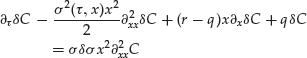
To express δ J in terms of δ σ, an adjoint state function P is introduced as the solution to the adjoint problem: Find the function P such that ![]() and for
and for ![]() ,
,
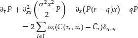
where ![]() is an arbitrary time greater than
is an arbitrary time greater than ![]() and in the right-hand side, the
and in the right-hand side, the ![]() denote Dirac functions in time and strike at
denote Dirac functions in time and strike at ![]() . The meaning of (61) is the following:
. The meaning of (61) is the following:
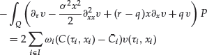
where ![]() , and v is any function such that
, and v is any function such that ![]() with
with ![]() and
and ![]() . Taking v = δ C in (62) and using (60), one finds
. Taking v = δ C in (62) and using (60), one finds
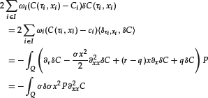
We have worked in a formal way, but all the integrations above can be justified. This leads to the estimate
![]()
which implies that J is differentiable, and that its differential at point σ is given by
![]()
where P(σ) satisfies (61), and C(σ) satisfies (58). We see that the gradient of J can be evaluated. When (58) is discretized with, for example, finite elements, all that has been done can be repeated with a discrete adjoint problem, and the gradient of the functional can be evaluated in the same way. Let us stress that the gradient ![]() is computed exactly, which would not be the case with, for example, a finite difference method.
is computed exactly, which would not be the case with, for example, a finite difference method.
Local volatility can also be calibrated with American options, but it is not possible to find the analogue of Dupire’s equation. Thus, in the context of a least square approach, the evaluation of the cost function requires the solution of #I variational inequalities, which is computationally expensive (see Achdou and Pironneau, 2005). In this case, it is also possible to find the necessary optimality conditions involving an adjoint state (see Achdou, 2005).
Appendix: Proof of (21)
First, from the definition (15) of p we have, for any stopping time ![]() ,
,
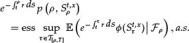
where ![]() denotes the set of stopping times
denotes the set of stopping times ![]() such that
such that ![]() . Then it is possible to show that (see, for instance, Karatzas and Shreve, 2010, Eq. (D.7)), for any stopping time
. Then it is possible to show that (see, for instance, Karatzas and Shreve, 2010, Eq. (D.7)), for any stopping time ![]() ,
,
We obtain from (64) the decreasing property: For all stopping times ![]() , such that
, such that ![]() ,
,
We deduce from (63) that, for any ![]() ,
,
where the last identity comes from the definition (20) of ![]() . Then, for any stopping time
. Then, for any stopping time ![]() , we have (by decomposing on the events
, we have (by decomposing on the events ![]() and
and ![]() ), and using (66) for
), and using (66) for ![]() ):
):
![]()
Hence, by taking the supremum over all the stopping times ![]() ,
,
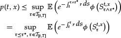
By (15), the right-hand side of (67) is bounded from above by p(t,x), and thus we obtain the equality
In fact the supremum in (68) is reached only for ![]() a.s.. Indeed, for
a.s.. Indeed, for ![]() , if
, if ![]() and
and ![]() , we have, by the definition of
, we have, by the definition of ![]() ,
, ![]() . This concludes the proof of (21).
. This concludes the proof of (21).
KEY POINTS
- When a deterministic method is available to price an option, it is generally more efficient than a brute force Monte Carlo algorithm.
- Deterministic techniques are usually more involved to implement than stochastic approaches and typically require specific developments for each targeted pricing problem.
- Deterministic approaches are particularly useful for nonlinear problems (including the pricing of American options and portfolio optimization) and for calibration.
- Future research subjects for such approaches include the development of efficient discretization methods for high-dimensional problems, and the combination of deterministic and stochastic approaches to take advantage of both techniques (using variance-reduction techniques or predictor-corrector methods, for example).
NOTES
1. Notice that the same equation has been considered by Vecer (2001) using some financial arguments.
2. http://www-rocq.inria.fr/mathfi/Premia/index.html
4. More precisely, the interpolating operator ![]() should also satisfy
should also satisfy ![]() everywhere as soon as
everywhere as soon as ![]() for all k, j.
for all k, j.
5. A good initial guess is indeed the vector α obtained at the previous time iteration.
6. F is slantly differentiable if there exist C>0 and a matrix G(x) such that ![]() ,
, ![]() and F(x+h) = F(x)+G(x+h)h+o(h) as
and F(x+h) = F(x)+G(x+h)h+o(h) as ![]() . Here G(x) can be defined by
. Here G(x) can be defined by ![]() if
if ![]() , and
, and ![]() otherwise.
otherwise.
7. Such a problem is called a linear complementarity problem.
REFERENCES
Achdou, Y. (2005). An inverse problem for a parabolic variational inequality arising in volatility calibration with American options. SIAM J. Control Optim. 43, 5: 1583–1615.
Achdou, Y., and Pironneau, O. (2005). Computational methods for option pricing. Frontiers in applied mathematics. Society for Industrial & Applied Mathematics 30.
Achdou, Y., Hecht, F., and Pommier, H. (2008). Space-time a posteriori error estimates for variational inequalities. Journal of Scientific Computing 37: 336–366.
Achdou, Y., and Pironneau, O. (2009). Partial differential equations for option pricing. In P. G. Ciarlet, ed., Handbook of Numerical Analysis, Vol. XV, Special Volume: Mathematical Modeling and Numerical Methods in Finance, Guest Eds., Alain Bensoussan and Qiang Zhang. Netherlands: North-Holland, 369–495.
Ammar, A., Mokdad, B., Chinesta, F., and Keunings, R. (2002). A new family of solvers for some classes of multidimensional partial differential equations encountered in kinetic theory modeling of complex fluids. Journal of Non-Newtonian Fluid Mechanics 139: 153–176.
Avellaneda, M., Levy, A., and Paras, A. (1995). Pricing and hedging derivative securities in markets with uncertain volatilities. Applied Mathematical Finance 2: 73–88.
Barles, G. (1994). Solutions de viscosité des équations de Hamilton-Jacobi, vol. 17 of Mathematics & Applications. Paris: Springer-Verlag.
Barles, G., Daher, C., and Romano, M. (1995). Convergence of numerical schemes for parabolic equations arising in finance theory. Mathematical Models and Methods in Applied Sciences 5, 1: 125–143.
Barles, G., and Souganidis, P. E. (1991). Convergence of approximation schemes for fully nonlinear second order equations. Asymptotic Analysis 4, 3: 271–283.
Bensoussan, A., and Lions, J.-L. (1978). Applications des inéquations variationnelles en contrôle stochastique. Méthodes Mathématiques de l’Informatique, No. 6. Paris: Dunod.
Beylkin, G., and Mohlenkamp, M. J. (2002). Numerical operator calculus in higher dimensions. Proceedings of the National Academy of Sciences 99, 16: 10246–10251.
Black, F., and Scholes, M. (1973). The pricing of options and corporate liabilities. Journal of Political Economy 81: 637–654.
Bokanowski, O., Maroso, S., and Zidani, H. (2009). Some convergence results for Howard’s algorithm. SIAM Journal of Numerical Analysis 47, 4: 3001–3026.
Boyaval, S., Le Bris, C., Lelièvre, T., Maday, Y., Nguyen, N. C., and Patera, A. T. (2010). Reduced basis techniques for stochastic problems. Archives of Computational Methods in Engineering 17, 4: 435–454.
Brennan, M. J., and Schwartz, E. S. (1977). The valuation of the American put option. Journal of Finance 32: 449–462.
Bungartz, H. J., and Griebel, M. (2004). Sparse grids. Acta Numerica 13: 147–269.
Capuzzo-Dolcetta, I., and Falcone, M. (1989). Discrete dynamic programming and viscosity solutions of the Bellman equation. Annales de l’Institut Henri Poincaré, Analyse Non Linéaire 6: 161–183.
Carr, P., Geman, H., Madan, D., and Yor, M. (2002). The fine structure of asset returns: An empirical investigation. Journal of Business 75, 2: 305–332.
Cont, R., and Tankov, P. (2003). Financial Modelling with Jump Processes. Boca Raton: Chapman and Hall.
Cont, R., and Tankov, P. Nonparametric calibration of jump-diffusion option pricing models. Journal of Computational Finance 7, 3: 1–49.
Courant, R., Friedrichs, K., and Lewy, H. (1967). On the partial difference equations of mathematical physics. IBM Journal of Research and Development 11: 215–234.
Cox, J., Ross, S., and Rubinstein, M. (1979). Option pricing: A simplified approach. The Journal of Financial Economics 7: 44–50.
Crandall, M. G., Ishii, H., and Lions, P.-L. (1992). User’s guide to viscosity solutions of second order partial differential equations. Bulletin of the American Mathematical Society (N.S.) 27, 1: 1–67.
Crandall, M. G., and Lions, P.-L. (1984). Two approximations of solutions of Hamilton-Jacobi equations. Mathematics of Computation 43, 167: 1–19.
Dubois, F., and Lelièvre, T. (2005). Efficient pricing of Asian options by the PDE approach. Journal of Computational Finance 8, 2: 55–64.
Duffie, D. (1992). Dynamic Asset Pricing Theory. Princeton: Princeton University Press.
Dupire, B. (1994). Pricing with a smile. Risk, 18–20.
El Karoui, N. (1981). Les aspects probabilistes du contrôle stochastique. In Ninth Saint Flour Probability Summer School—1979 (Saint Flour, 1979), vol. 876 of Lecture Notes in Math., pp. 73–238. Berlin: Springer.
Ern, A., Villeneuve, S., and Zanette, A. (2004). Adaptive finite element methods for local volatility European option pricing. International Journal of Theoretical and Applied Finance 7, 6: 659–684.
Falcone, M., and Ferretti, R. (1994). Discrete time high-order schemes for viscosity solutions of Hamilton-Jacobi-Bellman equations. Numerische Mathematik 67, 3: 315–344.
Fouque, J.-P., Papanicolaou, G., and Sircar, R. (2000). Derivatives in Financial Markets with Stochastic Volatility. Cambridge: Cambridge University Press.
Heston, S. (1993). A closed form solution for options with stochastic volatility with application to bond and currency options. Review with Financial Studies 6: 327–343.
Hintermuüller, M., Ito, K., and Kunisch, K. (2002). The primal-dual active set strategy as a semi- smooth Newton method. SIAM Journal of Optimization 13, 3: 865–888 (electronic, 2003).
Howard, R. A. (1960). Dynamic Programming and Markov Processes. Cambridge, MA: The Technology Press of M.I.T.
Hull, J. C., and White, A. (1987). The pricing of options on assets with stochastic volatilities. Journal of Finance 42: 281–300.
Jaillet, P., Lamberton, D., and Lapeyre, B. (1990). Variational inequalities and the pricing of American options. Acta Applicandae Mathematicae 21, 3: 263–289.
Jakobsen, E. R. (2003). On the rate of convergence of approximation schemes for Bellman equations associated with optimal stopping time problems. Mathematical Models and Methods in Applied Sciences 13, 5: 613–644.
Karatzas, I., and Shreve, S. E. (1991). Brownian Motion and Stochastic Calculus, 2nd ed. New York: Springer-Verlag.
Karatzas, I., and Shreve, S. E. (2010). Methods of Mathematical Finance. New York: Springer-Verlag.
Kushner, H. J., and Dupuis, P. (2001). Numerical methods for stochastic control problems in continuous time. Applications of Mathematics, Vol. 24. New York: Springer-Verlag.
Lamberton, D., and Lapeyre, B. (1997). Introduction au calcul stochastique appliqué à la finance. Ellipses, Paris.
Le Bris, C., Lelièvre, T., and Maday, Y. (2009). Results and questions on a nonlinear approximation approach for solving high-dimensional partial differential equations. Constructive Approximation 30: 621–651.
Lions, P.-L., and Mercier, B. (1979). Splitting algorithms for the sum of two nonlinear operators. SIAM Journal on Numerical Analysis 16, 6: 964–979.
Merton, R. C. (1973). Theory of rational option pricing. Bell Journal of Economics and Management Science 4: 141–183.
Merton, R. C. (1976). Option pricing when underlying stock returns are discontinuous. Journal of Financial Economics 3: 125–144.
Nouy, A. (2009). Recent developments in spectral stochastic methods for the numerical solution of stochastic partial differential equations. Archives of Computational Methods in Engineering 16: 251–285.
Øksendal, B., and Reikvam, K. (1998). Viscosity solutions of optimal stopping problems. Stochastics and Stochastics Reports 62, 3–4: 285–301.
Pham, H. (2006). Optimisation et Contrôle Stochastique Appliqués à la Finance. Springer Verlag, Berlin.
Pham, H. (1998). Optimal stopping of controlled jump diffusion processes: A viscosity solution approach. Journal of Mathematical Systems, Estimation, and Control 8, 1: 27 pp. (electronic).
Pironneau, O. (2007). Dupire-like identities for complex options. Comptes Rendus de l’Académie des sciences, Série I 344: 127–133.
Quarteroni, A., and Valli, A. (1997). Numerical Approximation of Partial Differential Equations. Springer, Berlin.
Rogers, L. C. G., and Shi, Z. (1995). The value of an Asian option. Journal of Applied Probability 32: 1077–1088.
Saad, Y. (2003). Iterative methods for sparse linear systems. Society for Industrial & Applied Mathematics.
Santos, M. S., and Rust, J. (2004). Convergence properties of policy iteration. SIAM Journal on Control and Optimization 42, 6: 2094–2115.
Stein, E., and Stein, J. (1991). Stock price distributions with stochastic volatility: An analytic approach. Review of Financial Studies 4, 4: 727–752.
Temlyakov, V. N. (2008). Greedy approximation. Acta Numerica 17: 235–409.
Thompson, G. W. P. (1999). Fast narrow bounds on the value of Asian options. Working paper, Judge Institute U. of Cambridge, 1999.
van der Pijl, S. P., and Osterlee, C. W. (2011). An ENO-based method for second order equations and application to the control of dike levels. Journal of Scientific Computing, in press.
Věcěr, J. (2001). A new PDE approach for pricing arithmetic average Asian options. Journal of Computational Finance 4, 4: 105–113.
von Petersdoff, T., and Schwab, C. (2004). Numerical solutions of parabolic equations in high dimensions. Mathematical Modelling and Numerical Analysis 38: 93–128.
Wilmott, P., Dewynne, J., and Howison, S. (1993). Option Pricing: Mathematical Models and Computation. Oxford: Oxford Financial Press.
Zvan, R., Forsyth, P. A., and Vetzal, K. (1998). Robust numerical methods for PDE models of Asian options. Journal of Computational Finance 1, 2: 39–78.