Managing the Model Risk with the Methods of the Probabilistic Decision Theory

VACSLAV S. GLUKHOV, PhD

Head of Quantitative Strategies and Data Analytics, Liquidnet Europe Ltd, London, United Kingdom

Practical applications of financial models require their parameters to be given concrete numerical values. These values are typically fitted to empirical data to ensure that the model predictions match historical observations. Parameter values obtained by such fitting procedures never propagate into the future unchanged: Tracing the model’s steps back in time, we find that its parameters are always more or less in error. The convention is that predictions made by the model are better if its parameters are known with better precision.

Thus, financial models are always in error—to an extent. Additional variability of actual outcomes due to models themselves, or model risks, can be loosely associated with Knightian uncertainty. Methods of Bayesian inference estimate the extent of this uncertainty, whereas the utility theory helps evaluate relative costs of decisions made under this uncertainty. Probabilistic decision theory, which combines Bayesian inference with the concept of utility, is the natural and powerful tool for handling intrinsic risks of financial models. The purpose of this chapter is to demonstrate how it works in practice.

AN OUTLINE OF PROBABLISTIC DECISION THEORY

As McKay (2008) cleverly puts it, probabilistic decision theory is trivial—apart from computational details. It has its roots in the Bayesian inference and in the concept of the utility, or the loss, function. Bayesian inference with its pure probabilistic methods is now gaining its long-deserved position in financial applications.

The utility function that maps the outcomes of possible decisions d onto the value space (or, conversely, the cost space) V is a concept that embodies personal choice and individual risk preferences. In its simplest form, the cost space is one-dimensional. This makes it possible to order decisions by their costs. The decision that has a minimum cost (or a maximum value) is the best decision in the sense of the utility function U.

We will proceed to the formulation of the probabilistic decision-making theory according to Jaynes (2003) and McKay (2008). If E(.) is the expectation, d is the decision, U(d) is the utility function of the decision, θ is the probable future state of the world, and P(θ, d) is the probability of θ, possibly influenced by the decision, then the optimal decision that maximizes the expectation of the utility function is

In exact sciences, the states of the world θ are represented by objective quantities such as temperature, energy density, barometric pressure, acidity, and the like. Measurements of these quantities are subject to errors whose distribution is often fairly well known from the theory of the underlying physical process. For example, in electronics, the probability of an error of a weak signal is closely linked to the ambient temperature, which is an objective and measurable quantity. In engineering the contribution of side factors can often be accounted for and controlled for to a great degree. The existence of the underlying theory capable of quantitative description of the noise and other factors greatly simplifies decision making under uncertainty in engineering and in other exact sciences in comparison with financial applications.

It is customary to employ the same reasoning in finance. When we talk about “more precise prediction of volatility” or “an accurate correlation coefficient” we implicitly assume that these quantities and parameters in finance are objective. They are not. Not unless we supply an underlying micro-model derived from the first principles, as we routinely do in exact sciences. In contrast, states of the world θ in finance are not inexact measurements of some “true quantities” linked to natural phenomena. Rather, they are mental constructs, which help us reason about financial phenomena—with more or less success. In financial observations, controlling for other factors is not possible, so the concept of ceteris paribus does not exist in nontrivial cases of any practical significance. It is better to think about states of the world in financial applications as relatively stable properties of markets and financial instruments. Depending on circumstances, such mental concepts as volatility, correlations, liquidity, expected time to default, and so on can be regarded as states of the world in finance.

States θ are functions of the model employed θ = θ (M). Given the set of observations Y and subjective priors I, each state θ is assigned a probability:

Being the function of the model, the data, prior beliefs, and, possibly, the decision, the probability of the state θ encapsulates all that is known to be relevant about the phenomenon under consideration.

Probabilistic inference, apart from very special cases, is often tractable only by computer techniques: P(θ |Y) has no analytical representation and must be ultimately sampled from the data.

The utility function U(θ, d) introduces the cost (or utility) of each decision in each state of the world. In academic research, one typically chooses a smooth and convex utility function. This should not necessarily be the case in the real world of financial applications where various smooth and nonsmooth constraints must be satisfied—such as risk tolerance, tax considerations, strict and soft budget constraints.

Note that except for the observable data, all other components in the probabilistic decision-making process are user-dependent—the model, the beliefs, and the utility preferences. In the world of subjective views, there is no universal truth, there are no unconditionally good or poor decisions. All decisions are ultimately conditional on personal preferences.

Let’s consider how it works in two simple financial applications: risk management of a simple portfolio and valuation of a risky bond.

MODEL RISK OF A SIMPLE PORTFOLIO

A portfolio manager considers creating an investment vehicle based on the instrument Y. The portfolio manager’s objective is to extract as much idiosyncratic alpha as possible from Y while reducing the risks associated with the factor X. Instruments highly correlated with X are available for short selling, or instruments highly negatively correlated with X are available for purchase. There are costs associated with these actions. The portfolio manager has an amount of capital equal to C and access to an abundant and relatively low-risk security Z, which can be used to preserve capital. The objective is to meet investment goals G(T), which include return on capital and risk parameters over a definite time horizon T.

The portfolio manager’s decisions are based on prior beliefs and the data. The portfolio manager begins splitting capital among X, Y, and Z such that

The allocation of capital is determined by the optimization of the utility function given by:

Expectations of future returns depend on the model parameters. In the Bayesian decision framework, the distributions of these parameters are important:

In the list, the first risk can be understood as the true risk; the last three risks are the model risks or uncertainty.

Consider the model that links contemporaneous data yt and xt in a linear fashion:

This model is a simplification of the industry-standard factor risk model and is akin to that used in the capital asset pricing theory (Sharpe, 1964), where a similar relationship is defined implicitly, or Fama and French (1992), where several factors are used.

The probability of observing the datum yt given the unknown parameter of the model β is

It is customary to select a normal model of the idiosyncratic noise as it is a well-behaving distribution that falls off very fast and which for this reason has all its moments well defined. This, in turn, assists in obtaining clear analytical results with helpful illustrative properties.

One needs to remember, however, that real financial noise is neither normal, nor log-normal: It has fat tails, which can be so poorly behaving that the distribution may not even have its first moment well defined. In the probabilistic decision framework, it is almost never possible to obtain a neat analytical expression for the final result. Consequently, the advantages of the normally distributed noise fade in comparison with more realistic models. Another advantage of the probabilistic framework is that one can easily compare evidence in favor of or against any conceivable model. In the presentation here, we retain the normalcy of the residual noise, bearing in mind that it is used for the sole purpose of illustrating the main idea.

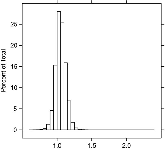
Figure 1 Distribution of β of Daily Price Changes over Three Years for Microsoft Corporation (MSFT) and the S&P 500 EFT (SPY)

Noise values being identically distributed and independent, which again is not a requirement for the probabilistic decision theory, the probability of observing the data set consisting of N points is

It is easier to see the properties of the likelihood function by taking the logarithm:

As a function of β, the log-likelihood attains a maximum at the same point where the ordinary least squares (OLS) method finds its optimum value of . Contrary to the OLS, which boils down all the available data to one number, which is then taken as a real objective quantity, the probabilistic framework retains more information about the relationship between Y and X, thereby preserving it in the distribution P(β |XY).

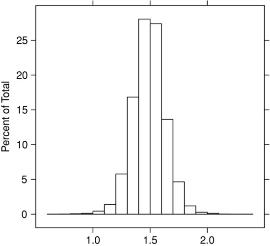
In Figure 1 we show the distribution of β, P(β |XY), when the dependent instrument Y is the daily change in the price of Microsoft Corporation stock and the independent instrument X is the daily price change of the exchange-traded fund SPY corresponding to the Standard & Poor’s 500 index. Three years of daily data are used in the estimates of P(β |XY). In Figure 2 the same amount of data is used to estimate P(β |XY) when Y is the daily change in the price of the stock of a natural resource company, the Mosaic Company, and X is, again, the set of contemporaneous daily price changes in SPY.

Figure 2 Distribution of β of Daily Price Changes over Three Years for the Mosaic Company (MOS) and the S&P 500 ETF

Having obtained distributions of the model parameters β, μ, and σ from the data, the portfolio manager blends likelihoods with opinions about the distribution of the residual returns. The portfolio manager’s alpha model is that the expectation of daily returns of Y is μ 0 with the confidence band : . Combined with subjective opinions, the idiosyncratic distribution is again, normal:

In order to overcome the evidence extracted from the data and given by μ, the portfolio manager’s confidence must be greater than the confidence range of the data: The portfolio manager’s confidence is high, that is, when , the posterior expectation of alpha is governed by the portfolio manager’s prognosis. In the opposite case, the data are trusted more than the portfolio manager’s judgment.

The portfolio manager sets risk preferences with the utility function

Taking the expectations over one period T = 1 we obtain:

Here

First, we focus on the problem of optimum allocation when there is no hedging: wx = 0, μ x = 0. Define the certainty equivalent (CE) of the investment in Y and Z as such guaranteed change in C that results in the same utility as a risky investment in Y and Z. Mathematically, it is defined as the inverse of the utility function:

For the exponential utility function we obtain

Adopting and integrating expected utility over the model parameter β, we finally arrive at

The first three terms in this equation represent the certainty equivalent of the investment without the risk model β 0 = 0 and without the model risk . The optimal fraction of the capital invested in Y is a well-known expression (see, for example, Merton, 1969)

In this case, the fraction invested in the risky instrument is proportional to the portfolio manager’s risk tolerance and inversely proportional to the instrument’s idiosyncratic risk, which, in the absence of any model, is the total risk of the instrument.

Introduction of the risk model without uncertainty results in the obvious extension:

Here is, again, the total risk of Y as given by the model, split into the idiosyncratic part and the part coming from the influence of X.

When , the last two terms in the equation for represent the model risk. In some situations, the term can be thought of as the contribution to the expected variance due to the model risk. Indeed, if (i.e., when the risk tolerance is much greater than possible risk associated with the factor X) in the expression for the certainty equivalent, the model risk is simply added to the total risk:

In this expression, the last term is proportional to the magnitude of the expression in parentheses and is small in comparison with the preceding terms.

The contribution of the model risk is not so obvious in a general case. Clearly, when , the model risk significantly affects optimal allocations.

Position Hedging

Now the portfolio manager aims to reduce the influence of the factor X on the variability of returns. The portfolio manager adds a position in X to the portfolio. Weight wx allocated to X is chosen to maximize CE. Positive weight corresponds to a long position in X, whereas a negative weight corresponds to a short position or its equivalent. In the case when X is the daily performance of the Standard & Poor’s 500 market index, a short position can be roughly replicated by taking a long position in an exchange-traded fund (ETF) whose daily returns correspond by design to the inverse—up to a constant factor—of the daily performance of the S&P 500 index.

The certainty equivalent of the portfolio is

The first two terms in this expression are the idiosyncratic alpha and risk of the instrument Y.

The third term introduces the risk associated with the portfolio returns dependence on X. Let’s take a closer look at it. Its structure is similar to the term describing the idiosyncratic risk: variance of the portfolio due to X divided by the portfolio manager’s risk tolerance. In the third term, contribution from the risk model comes in two forms. In the numerator wx+β 0wy is the total weight of X in the portfolio: the sum of the weight of the position in X, wx and the estimate of the contribution from exposure to X of the position in Y, β 0wy. The fact that the total contribution of X is the same as in the standard portfolio theory is purely accidental and is due to the choice of the model distribution of β.

In the denominator, the portfolio manager’s risk tolerance is augmented by a factor that depends on the uncertainty of β:

This term being less than unity, uncertainty effectively reduces the portfolio manager’s risk tolerance.

The fourth term is the contribution to CE from the model risk. Terms associated with the model risk indicate that when the uncertainty of the model approaches a critical value the portfolio becomes unfeasible unless wy is sufficiently small.

In the absence of a risk model optimal allocations maximizing of the portfolio are

When the risk model is present, but the uncertainty of the model is much bigger than its prediction , we obtain another useful result:

In this case the optimal allocation in Y is determined by the total risk of the instrument composed of the idiosyncratic risk and the uncertainty of the model.

When the risk model is present and is absolutely precise the usual hedging ratio completely eliminates the dependency of portfolio returns and their CE on X—the result conventionally obtained in the traditional formulation of the risk management problem.

From the probabilistic point of view, however, an absolutely precise model is nonsensical. Moreover, situations when both the model’s optimal parameters and the uncertainty of the parameters are of the same order of magnitude are most likely to occur in real applications.

Contribution from the risk model and from the uncertainty of the model become separated and especially simple when the portfolio manager’s risk tolerance is sufficiently large, :

Note that there is no combination of the instruments Y and X that can eliminate the effect of X. That the effect of the instrument X may never be eliminated completely is a better depiction of the everyday experience of the portfolio manager. Probabilistic decision theory accounting for the model risk, however, gives a reasonable indication of what the portfolio manager can expect from such or another composition of the portfolio when its components are mutually dependent.

In more complicated settings, once the portfolio manager introduces the costs of hedging, the decision whether to hedge or not comes naturally as the consequence of the interplay between the value of hedging and the costs. Let y|wxC| = y|β 0wyC| be the cost associated with the hedge. Then one should hedge the position if

Hedging is justified if the model risk of the hedge plus the cost of implementing the model is smaller than the original risk that the hedge is meant to reduce.

In the equation above all quantities are evaluated from the data and the subjective prior beliefs using the methods of the Bayesian inference. Even when the model and the model parameters are relatively stable, the decision whether to hedge or not to hedge depends on the portfolio manager’s risk tolerance, which in turn can be represented by a combination of external constraints, or be inferred from another model.

A portfolio manager can readily extend the methodology of the preceding sections to more complicated cases of many interrelated instruments and many factors. The probability distribution of the correlation matrix, however, will not necessarily appear in the calculations in place of the probability distribution of β: Noise models that have no concept of second or higher moments completely rule out correlation matrices in the calculations. Moreover, these distributions naturally lead to decisions being determined by a few extreme outliers. Fortunately, even pathological noise distributions, which seem to be the norm rather than an exception in finance, are treated equally well by the methods of the probabilistic decision theory, which is designed to incorporate all available data plus the portfolio manager’s preferences and constraints.

In the next section we will address a problem of the model risk in an investment when the risk profile is different from that of an investment in an equity portfolio.

INVESTMENT IN A RISKY BOND

Let P be the face value of the zero-coupon bond, r the benchmark rate over the period of interest, ρ the multiplicative spread rate for the bond, so that

is the current fair or market price of the bond, possibly unknown. An alternative investment vehicle Z is available as in the previous section, the rate of return for this instrument being rz.

Let there be two possible states of the world. In the first state the bond is redeemed at the face value at the end of the period. In the second state of the world the bond is redeemed at Py. The situation when Py = 0 is possible, in which case the investment is a total loss. If the investor purchases N units of the risky bond and the remainder of the capital is preserved in the alternative vehicle, then, at the end of the period, the investor’s capital is

In the traditional formulation the investment is justified if the expected return on capital when N>0 is greater than the expected return when N = 0. This translates into the following expression, which links all the input data of the problem and the unknown value of the bond:

This traditional approach is a reasonably good approximation under certain conditions. A much richer view along with the set of quantitative tools is required in a general case.

From the probabilistic decision theory viewpoint, the probabilities and other relevant parameters entering the decision-making process must be inferred from the model, from the data, and from the investor’s prior beliefs, and are best represented by distributions of possible states of the world. We consider now a simple one-parametric risk model and show how the model risk contributes to the decision process.

Parameter Inference in the Bernoulli Model

In the Bernoulli-like model, the investment vehicle under consideration belongs to a class of essentially similar bonds. They are financial obligations issued by debtors facing essentially the same economic (financial, market, etc.) conditions. Given these conditions, it is customary to assume that the failure of each instrument is a random event. Failures in the class occur with the same probability pd per unit time, which, for simplicity, will coincide in our analysis with the maturity time of the instrument.

The model of the random process, the empirical data, and the investor’s prior beliefs determine all that we know about the model parameter pd.

Assume that the empirical data are the sample of N observations of the class, and m is the number of cases when a debtor defaults. Adopting a beta-distribution of the model parameter, we obtain the following posterior distribution given the data and the prior beliefs:

where

and α 0, β 0 are the parameters representing the investor’s prior beliefs. In the prior distribution, α 0 can be interpreted as number of cases of default and β 0 is the number of cases when the bond was repaid in full. The prior distribution’s parameters can come from the investor’s own experience, or from the consensus of experts, or be inferred from agency ratings. The magnitude of α 0, β 0 versus n, m determines the relative weight the investor assigns to prior beliefs. Prior beliefs dominate the data when .

Figure 3 Distribution of the Probability of Default pd

Note: Prior distribution is defined by α 0 = 2, β 0 = 11. Newly arriving data follow the new probability .

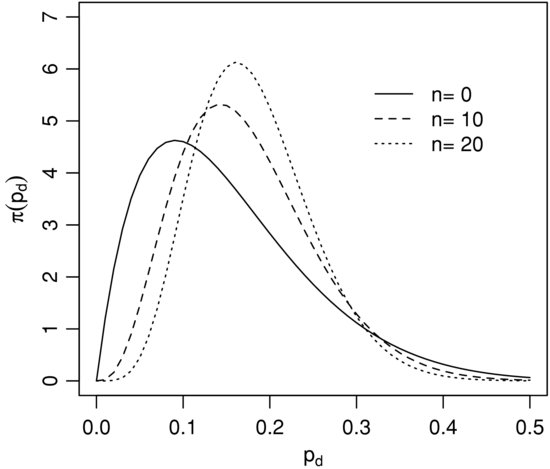
In Figure 3, the investor’s prior beliefs follow the prior probability of default 0.1. Parameters of the prior distribution are α 0 = 2, β 0 = 11. The newly arriving data point to the probability of default 0.2. Observe the change in the shape of the distribution: Its mode moves from to as the new data gradually overcome the investor’s prior beliefs. Note that the model risk—the width of the distribution—remains relatively high.

In the Bayesian perspective, the distribution of the probability of default is a convenient vehicle that carries all that the investor knows from the set of observations and the investor’s prior beliefs: what is the most probable state of the world and what is the spread of possible states of the world given the investor’s choice of the model of the world.

The rich framework offered by the Bayesian inference of the probability of default consequently brings in a rich set of valuation methods that naturally account for the model risk. In the next sections we will study the valuation effects of the risk of models.

Model Risk Contribution to the Fair Price of the Bond

First, we obtain an interesting estimate of the model risk contribution to the fair price of the bond under the assumption of the infinite risk tolerance. This is a degenerate case most closely resembling the traditional formulation. The utility function is linear if the investor’s risk tolerance is infinite.

We obtain formally:

Assume that the sample size is N of which there are m defaults. A flat prior distribution describes an investor who initially is ignorant. Expectation of the probability of default is then governed by the rule of succession (originally developed by Laplace):

The difference between this posterior expectation and the naïve probability of default pd = m/n is the contribution of the model risk to the fair price of the bond:

For example, if the naïve default rate estimate is 0.1 and it is based on 100 observations, the contribution of the model risk to the fair price of the bond can be as big as 78 basis points—not an insignificant amount: The model risk can be a substantial contributor to the overall risk of the investment. Thus, the sampling risk and the prior beliefs bias yield a substantial contribution to the overall risk of the investment.

Even in the simplest Bernoulli-like model, the contribution of the model risk to the value of the bond is nonnegligible. This contribution is especially pronounced when the probability of default is small.

Now we will proceed to a case when the investor’s risk tolerance is not infinite. We will show that average probabilities are likely insufficient for making an informed investment decision. Relying on just expected probabilities can result in catastrophic consequences for the investor.

Model Risk of Agency Ratings

Currently financial regulators recommend that expected losses be quantified as the expected probability of default times the exposure at default (see Basel, 2008). Consequently, credit scoring and rating agencies aim at developing models that generate expected probabilities of default. These models are calibrated by minimizing the difference between predicted and empirically observed probabilities of default (see, for example, Korablev and Dwyer, 2007). From the preceding section, it follows that the average rates based on thousands of credit events used in the calibration of the agency model alone are insufficient for making investment decisions concerning a portfolio of an arbitrary, possibly small, subset of instruments. Moreover, the naïve probability of default is likely to be useless in the valuation of a singular derivative instrument, such as a credit default swap (CDS). For a financial practitioner it is important to know, however, that agencies possess and disclose substantially more information than ratings, scoring, or expected probabilities alone. We will now discuss briefly how this information is used in the probabilistic decision framework.

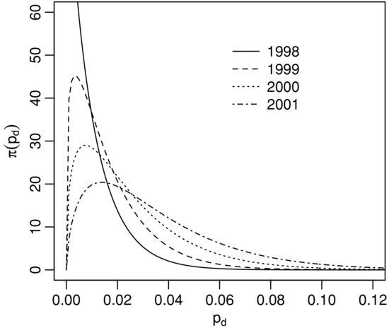
Korablev and Dwyer (2007) report that for a certain group of companies the Moody’s KMV EDF™ model was predicting 2.5% as the mean probability of default in 2002. The value of 1.8% was actually observed. The 10 and 90 percentiles of the distribution of predicted rates were 0.5% and 5.4%. This information is sufficient to reconstruct the parameters of the beta-distribution discussed earlier. An approximate match is α = 1.12, β = 56.35. In Figure 4 we show the set of implied distributions for the four years preceding 2002. The inferred distribution for the year 2002 is almost identical to that for 2000.

Figure 4 Implied Distribution of the Probability of Default pd According to the Moody’s Data for 1998, 1999, 2000, and 2001

We will now show how the inferred model of the probability of default is used in the decision-making process.

It appears from the following analysis that due to idiosyncrasies of the distribution of the probability of default, the effects of the model risk can be profound, even catastrophic. Describe the investor’s risk preferences with the following disutility function:

This function describes an investor who is progressively reluctant to tolerate deviations from the expected probability of default when these deviations exceed . Note that disutility of positive deviations from the expected value is growing exponentially, while the beta-distribution of pd falls off around its mode much slower, approximately as a power function. Using a beta-distributed probability of default , we find for the certainty equivalent

where F(a, b, z) is the regularized confluent hypergeometric function (Weisstein, 2010). The certainty equivalent of can be interpreted as an equivalent certain probability of default, which supplies the same value for the investor as the uncertain probability of default—given the investor’s risk preferences.

In the limit

At high tolerances CE(pd) coincides with the mean naïve probability of default. As the investor’s risk tolerance decreases, however, the certainty equivalent grows more and more rapidly. A plot of the exact certainty equivalent probability of default as the function of the model risk tolerance is shown in Figure 5. The parameters of the distribution are α = 1.45 and β = 15, and the dashed line is the asymptote α /(α +β).

Figure 5 versus Risk Tolerance

Note: Dashed line is the asymptote value α /(α +β), α = 1.45, β = 45

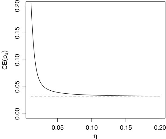
The catastrophic divergence of the certainty equivalent probability occurs at the values of the tolerance that are close to the width of the distribution : At the tolerance level the CE(pd) is as big as 0.23, more than seven times the naïve value of the probability. From the practical decision-making standpoint it means that if the investor accepts the price of the bond or associated instruments defined by the naïve probability 0.031, it is likely that the investor is grossly mistaken about the value of the bond given the investor’s risk tolerance and the model risk.

KEY POINTS

• Probabilistic decision theory is a blend of the probabilistic, also called Bayesian, inference and the concept of utility.
• In the probabilistic decision theory optimal decisions maximize the expected value of the user’s utility over all possible states of the world.
• Probabilities of the states of the world are inferred from the empirical data, the model, and the user’s beliefs.
• Uncertainty in the model parameters results in the model risk; a financial model that is free of the model risk is an exception.
• Practical consequences of the model risk are evaluated using the utility function.
• Model risk significantly augments optimal allocations in equity portfolios and can result in a prospective portfolio being ruled out.
• Valuation of a risky bond is significantly affected by the model risk; ratings and expected probabilities of default alone are likely insufficient for the decision-making process.
• Failure to account for the model risk can lead to catastrophic consequences for the investor.
• Unhandled or unknown model risk produces risk exposure that remains indeterminate.

REFERENCES

Basel Committee on Banking Supervision. (2008). Guidelines for Computing Capital for Incremental Risk in the Trading Book. Bank for International Settlements.

Fama, E. F., and French, K. (1992). The cross-section of expected stock returns. Journal of Finance 47, 2: 427–466.

Jaynes, E. T. (2003). Probability Theory: The Logic of Science. Cambridge: Cambridge University Press.

Korablev, I., and Dwyer, D. (2007). Power and Level Validation of Moody’s KMV EDF™ Credit Measures in North America, Europe and Asia. Moody’s KMV, September 10.

McKay, D.J.C. (2008). Information Theory, Inference and Learning Algorithms. Cambridge: Cambridge University Press.

Merton, R. C. (1969). Lifetime portfolio selection under uncertainty. Review of Economics and Statistics 51: 247–257.

Sharpe, W. F. (1964). Capital asset prices: A theory of market equilibrium under conditions of risk. Journal of Finance 19, 3: 425–442.

Weisstein, E. W. (2010). Regularized hypergeometric function. MathWorld: A Wolfram Web Resource. http://mathworld.wolfram.com/RegularizedHypergeometricFunction.html